Diverging length scale of the inhomogeneous mode-coupling theory: a numerical investigation

Grzegorz Szamel and Elijah Flenner Department of Chemistry, Colorado State University, Fort Collins, CO 80523
Abstract

Biroli et al.’s extension of the standard mode-coupling theory to inhomogeneous equilibrium states [Phys. Rev. Lett. 97, 195701 (2006)] allowed them to identify a characteristic length scale that diverges upon approaching the mode-coupling transition. We present a numerical investigation of this length scale. To this end we derive and numerically solve equations of motion for coefficients in the small q𝑞q expansion of the dynamic susceptibility χ𝐪(𝐤;t)subscript𝜒𝐪𝐤𝑡\chi_{\mathbf{q}}(\mathbf{k};t) that describes the change of the system’s dynamics due to an external inhomogeneous potential. We study the dependence of the characteristic length scale on time, wave-vector, and on the distance from the mode-coupling transition. We verify scaling predictions of Biroli et al. In addition, we find that the numerical value of the diverging length scale qualitatively agrees with lengths obtained from four-point correlation functions. We show that the diverging length scale has very weak k𝑘k dependence, which contrasts with very strong k𝑘k dependence of the q0𝑞0q\to 0 limit of the susceptibility, χ𝐪=0(𝐤;t)subscript𝜒𝐪0𝐤𝑡\chi_{\mathbf{q}=0}(\mathbf{k};t). Finally, we compare the diverging length obtained from the small q𝑞q expansion to that resulting from an isotropic approximation applied to the equation of motion for the dynamic susceptibility χ𝐪(𝐤;t)subscript𝜒𝐪𝐤𝑡\chi_{\mathbf{q}}(\mathbf{k};t).

I Introduction

As a liquid is cooled, its dynamics not only gets slower but also becomes increasingly heterogeneous Ediger (2000); Richert (2002); Andersen (2005). Moreover, the characteristic size of regions with dynamics both significantly faster and significantly slower than the average dynamics grows upon cooling. This observation has led to the definition of a dynamic correlation length that measures the size of these so-called dynamic heterogeneneities. The dynamic correlation length was defined in terms of a four-point correlation function Lacevic et al. (2002) or a corresponding four-point structure factor Lacevic et al. (2003); Berthier (2004); Toninelli et al. (2005); Berthier et al. (2007).

While various four-point functions can readily be obtained from simulations (albeit they typically require more computational effort than the familiar two-point functions), they are difficult to access experimentally. To the best of our knowledge, four-point functions have been obtained directly only from experiments on granular systems Lechenault et al. (2008a, b). In a remarkable development, Berthier et al. Berthier et al. (2005) showed that derivatives of standard two-point functions with respect to thermodynamic variables like, e.g., density or temperature, could be related to integrals of three-point correlation functions. This opened a door to experimental investigations of the overall degree (the strength) of dynamic heterogeneity upon approaching the glass transition Dalle-Ferrier et al. (2007). It should be emphasized, however, that Berthier et al. could obtain the dynamic correlation length characterizing the spatial extent of dynamic heterogeneneities only by using additional assumptions that related the integrals of various three-point functions to characteristic length scales exhibited by these functions.

While theoretical understanding of the derivatives of two-point functions with respect to thermodynamic variables is limited, Biroli et al. Biroli et al. (2006) showed that the mode-coupling theory could be used to analyze a closely related quantity, a three-point susceptibility χq(k;t)subscript𝜒qk𝑡\chi_{\textbf{q}}(\textbf{k};t), which describes the change of the intermediate scattering function due to an inhomogeneous external potential. The advantage of this approach is that it allows one to evaluate a characteristic length scale which, up to that time, had remained hidden within the well-known mode-coupling framework. This was possible due to the fact that Biroli et al. considered a non-uniform external perturbation rather than a uniform change of density or temperature.

To analyze the three-point susceptibility Biroli et al. extended the standard mode-coupling theory to describe the time evolution of the intermediate scattering function of a system under the influence of an inhomogeneous external potential. They defined the three-point susceptibility χq(k;t)subscript𝜒qk𝑡\chi_{\textbf{q}}(\textbf{k};t) as a derivative of the intermediate scattering function with respect to a Fourier component of the external potential, U(𝐪)𝑈𝐪U(\mathbf{q}). Biroli et al. showed that upon approaching the mode-coupling transition both the q0𝑞0q\to 0 limit of the three-point susceptibility and a characteristic length defined through the small q𝑞q-dependence of χq(k;t)subscript𝜒qk𝑡\chi_{\textbf{q}}(\textbf{k};t) diverge. Moreover, they derived scaling predictions for the time-dependence of the characteristic length, and they found that this length grows as ta/2superscript𝑡𝑎2t^{a/2} in the early β𝛽\beta regime (here a𝑎a is the mode-coupling exponent describing approach of the intermediate scattering function to its plateau value) and then saturates in the late β𝛽\beta and α𝛼\alpha regimes. This was contrasted with the time dependence of the q0𝑞0q\to 0 limit of the three-point susceptibility which grows as tasuperscript𝑡𝑎t^{a} and tbsuperscript𝑡𝑏t^{b} in the early and late β𝛽\beta regimes, respectively (here b𝑏b is the so-called von Schweidler exponent of the mode-coupling theory describing departure of the intermediate scattering function from its plateau value), peaks around the α𝛼\alpha relaxation time, and then decays to zero. The strikingly different time-dependence of the characteristic length and the q0𝑞0q\to 0 limit of the three-point susceptibility was interpreted as an indication of changing fractal dimension of dynamic heterogeneities.

Biroli et al. derived only scaling predictions for the three-point susceptibility χq(k;t)subscript𝜒qk𝑡\chi_{\textbf{q}}(\textbf{k};t). They verified some of these predictions through a numerical analysis of a schematic model that completely disregards k𝑘k dependence. Here we present a numerical investigation of the small q𝑞q behavior of the three-point susceptibility and the associated characteristic length. We focus on the time and k𝑘k dependence of the length, and on its dependence on the distance to the mode-coupling transition.

We start with a definition of the three-point susceptibility χq(k;t)subscript𝜒qk𝑡\chi_{\textbf{q}}(\textbf{k};t) in Sec. II. Next, we postulate an expansion of the three-point susceptibility χq(k;t)subscript𝜒qk𝑡\chi_{\textbf{q}}(\textbf{k};t) in powers of 𝐪𝐪\mathbf{q} and derive equations of motion for the first few coefficients in this expansion (see Sec. III). We also present an alternative approach to a numerical evaluation of the characteristic length which is based on an isotropic approximation to the equation of motion (see Sec. IV). Next, in Secs. V and VII we describe the results of the numerical calculations based on the small q𝑞q expansion and the isotropic approximation, respectively. We finish with a summary and conclusions in Sec. VIII.

II Three-point susceptibility χq(k;t)subscript𝜒qk𝑡\chi_{\textbf{q}}(\textbf{k};t)

To obtain the equation of motion for the three-point susceptibility Biroli et al. Biroli et al. (2006) considered a Newtonian fluid subject to a periodic in space external potential, derived mode-coupling equation of motion for the intermediate scattering function of this inhomogeneous system, and then differentiated this equation with respect to the external potential. Subsequently, one of us has derived the equation of motion for the same three-point susceptibility for a Brownian system Szamel . Not surprisingly, the overdamped limit of the equation of motion derived by Biroli et al. coincides with the equation of motion derived starting directly from Brownian dynamics. In this work we will use the latter equation.

For a system subject to a non-uniform external potential the intermediate scattering function is not diagonal in the wave-vector,

F(𝐤1,𝐤2;t)=1Nρ(𝐤1;t)ρ(𝐤2)U.𝐹subscript𝐤1subscript𝐤2𝑡1𝑁subscriptdelimited-⟨⟩𝜌subscript𝐤1𝑡𝜌subscript𝐤2𝑈F(\mathbf{k}_{1},\mathbf{k}_{2};t)=\frac{1}{N}\left<\rho(\mathbf{k}_{1};t)\rho(-\mathbf{k}_{2})\right>_{U}. (1)

Here ρ(𝐤1;t)𝜌subscript𝐤1𝑡\rho(\mathbf{k}_{1};t) is the Fourier transform of the microscopic density,

ρ(𝐤1;t)=jei𝐤1𝐫j(t)𝜌subscript𝐤1𝑡subscript𝑗superscript𝑒𝑖subscript𝐤1subscript𝐫𝑗𝑡\rho(\mathbf{k}_{1};t)=\sum_{j}e^{-i\mathbf{k}_{1}\cdot\mathbf{r}_{j}(t)} (2)

with 𝐫j(t)subscript𝐫𝑗𝑡\mathbf{r}_{j}(t) being the position of the j𝑗jth particle at time t𝑡t. Furthermore, in Eq. (1) ρ(𝐤1)ρ(𝐤1;t=0)𝜌subscript𝐤1𝜌subscript𝐤1𝑡0\rho(\mathbf{k}_{1})\equiv\rho(\mathbf{k}_{1};t=0) and Usubscriptdelimited-⟨⟩𝑈\left<...\right>_{U} denotes the equilibrium average for a system subject to a static non-uniform external potential U𝑈U.

The three-point susceptibility χq(𝐤;t)subscript𝜒q𝐤𝑡\chi_{\textbf{q}}(\mathbf{k};t) is defined through an expansion of the intermediate scattering function in powers of a harmonic external potential U𝐪=U0ei𝐪𝐫subscript𝑈𝐪subscript𝑈0superscript𝑒𝑖𝐪𝐫U_{\mathbf{q}}=U_{0}e^{-i\mathbf{q}\cdot\mathbf{r}},

F(𝐤,𝐤1;t)=F(k;t)δ𝐤,𝐤1+χq(𝐤;t)(βU0)δ𝐤+𝐪,𝐤1+.𝐹𝐤subscript𝐤1𝑡𝐹𝑘𝑡subscript𝛿𝐤subscript𝐤1subscript𝜒q𝐤𝑡𝛽subscript𝑈0subscript𝛿𝐤𝐪subscript𝐤1F(\mathbf{k},\mathbf{k}_{1};t)=F(k;t)\delta_{\mathbf{k},\mathbf{k}_{1}}+\chi_{\textbf{q}}(\mathbf{k};t)\left(-\beta U_{0}\right)\delta_{\mathbf{k}+\mathbf{q},\mathbf{k}_{1}}+.... (3)

For a system with Brownian dynamics, the equation of motion for the three-point susceptibility χ𝐪(𝐤;t)subscript𝜒𝐪𝐤𝑡\chi_{\mathbf{q}}(\mathbf{k};t) has the following form:

tχ𝐪(𝐤;t)+D0k2S(k)χ𝐪(𝐤;t)subscript𝑡subscript𝜒𝐪𝐤𝑡subscript𝐷0superscript𝑘2𝑆𝑘subscript𝜒𝐪𝐤𝑡\displaystyle\partial_{t}\chi_{\mathbf{q}}(\mathbf{k};t)+\frac{D_{0}k^{2}}{S(k)}\chi_{\mathbf{q}}(\mathbf{k};t) (4)
+0t𝑑tMirr(k;tt)tχ𝐪(𝐤;t)superscriptsubscript0𝑡differential-dsuperscript𝑡superscript𝑀irr𝑘𝑡superscript𝑡subscriptsuperscript𝑡subscript𝜒𝐪𝐤superscript𝑡\displaystyle+\int_{0}^{t}dt^{\prime}M^{\mathrm{irr}}(k;t-t^{\prime})\partial_{t^{\prime}}\chi_{\mathbf{q}}(\mathbf{k};t^{\prime})
+0t𝑑tM𝐪χ(𝐤;tt)tF(|𝐤+𝐪|;t)superscriptsubscript0𝑡differential-dsuperscript𝑡subscriptsuperscript𝑀𝜒𝐪𝐤𝑡superscript𝑡subscriptsuperscript𝑡𝐹𝐤𝐪superscript𝑡\displaystyle+\int_{0}^{t}dt^{\prime}M^{\chi}_{\mathbf{q}}(\mathbf{k};t-t^{\prime})\partial_{t^{\prime}}F(|\mathbf{k}+\mathbf{q}|;t^{\prime})
=\displaystyle= 𝒮𝐪(𝐤;t)subscript𝒮𝐪𝐤𝑡\displaystyle\mathcal{S}_{\mathbf{q}}(\mathbf{k};t)

In Eq. (4) D0subscript𝐷0D_{0} is the diffusion coefficient of an isolated particle, S(k)𝑆𝑘S(k) denotes the static structure factor, Mirr(k;t)superscript𝑀irr𝑘𝑡M^{\mathrm{irr}}(k;t) is the irreducible memory function of mode-coupling theory,

Mirr(k;t)=superscript𝑀irr𝑘𝑡absent\displaystyle M^{\mathrm{irr}}(k;t)= (5)
nD02d𝐤1(2π)2[v𝐤(𝐤1,𝐤𝐤1)]2F(k1;t)F(|𝐤𝐤1|;t),𝑛subscript𝐷02𝑑subscript𝐤1superscript2𝜋2superscriptdelimited-[]subscript𝑣𝐤subscript𝐤1𝐤subscript𝐤12𝐹subscript𝑘1𝑡𝐹𝐤subscript𝐤1𝑡\displaystyle\frac{nD_{0}}{2}\int\frac{d\mathbf{k}_{1}}{(2\pi)^{2}}[v_{\mathbf{k}}(\mathbf{k}_{1},\mathbf{k}-\mathbf{k}_{1})]^{2}F(k_{1};t)F(|\mathbf{k}-\mathbf{k}_{1}|;t),

and Mχ(𝐪,k;t)superscript𝑀𝜒𝐪𝑘𝑡M^{\chi}(\mathbf{q},k;t) is defined as follows,

M𝐪χ(𝐤;t)=nD0k|𝐤+𝐪|d𝐤1(2π)3v𝐤(𝐤1,𝐤𝐤1)subscriptsuperscript𝑀𝜒𝐪𝐤𝑡𝑛subscript𝐷0𝑘𝐤𝐪𝑑subscript𝐤1superscript2𝜋3subscript𝑣𝐤subscript𝐤1𝐤subscript𝐤1\displaystyle M^{\chi}_{\mathbf{q}}(\mathbf{k};t)=\frac{nD_{0}k}{|\mathbf{k}+\mathbf{q}|}\int\frac{d\mathbf{k}_{1}}{(2\pi)^{3}}v_{\mathbf{k}}(\mathbf{k}_{1},\mathbf{k}-\mathbf{k}_{1}) (6)
×χ𝐪(𝐤1;t)F(|𝐤𝐤1|;t)v𝐤+𝐪(𝐤1+𝐪,𝐤𝐤1).absentsubscript𝜒𝐪subscript𝐤1𝑡𝐹𝐤subscript𝐤1𝑡subscript𝑣𝐤𝐪subscript𝐤1𝐪𝐤subscript𝐤1\displaystyle\times\chi_{\mathbf{q}}(\mathbf{k}_{1};t)F(|\mathbf{k}-\mathbf{k}_{1}|;t)v_{\mathbf{k}+\mathbf{q}}(\mathbf{k}_{1}+\mathbf{q},\mathbf{k}-\mathbf{k}_{1}).

In Eqs. (5-6) v𝐤(𝐤1,𝐤2)=𝐤^(𝐤1c(k1)+𝐤2c(k2))subscript𝑣𝐤subscript𝐤1subscript𝐤2^𝐤subscript𝐤1𝑐subscript𝑘1subscript𝐤2𝑐subscript𝑘2v_{\mathbf{k}}(\mathbf{k}_{1},\mathbf{k}_{2})=\hat{\mathbf{k}}\cdot(\mathbf{k}_{1}c(k_{1})+\mathbf{k}_{2}c(k_{2})) with 𝐤^=𝐤/k^𝐤𝐤𝑘\hat{\mathbf{k}}=\mathbf{k}/k, and n𝑛n is the density. The source term in Eq. (4), 𝒮𝐪(𝐤;t)subscript𝒮𝐪𝐤𝑡\mathcal{S}_{\mathbf{q}}(\mathbf{k};t), is given by

𝒮𝐪(𝐤;t)=subscript𝒮𝐪𝐤𝑡absent\displaystyle\mathcal{S}_{\mathbf{q}}(\mathbf{k};t)=
D0k2S(q)(1𝐤(𝐤+𝐪)k2S(|𝐤+𝐪|))F(|𝐤+𝐪|;t)subscript𝐷0superscript𝑘2𝑆𝑞1𝐤𝐤𝐪superscript𝑘2𝑆𝐤𝐪𝐹𝐤𝐪𝑡\displaystyle D_{0}k^{2}S(q)\left(1-\frac{\mathbf{k}\cdot(\mathbf{k}+\mathbf{q})}{k^{2}S(|\mathbf{k}+\mathbf{q}|)}\right)F(|\mathbf{k}+\mathbf{q}|;t)
+S(q)0t𝑑tMirr(k;tt)𝐤(𝐤+𝐪)|𝐤+𝐪|2tF(|𝐤+𝐪|;t).𝑆𝑞superscriptsubscript0𝑡differential-dsuperscript𝑡superscript𝑀irr𝑘𝑡superscript𝑡𝐤𝐤𝐪superscript𝐤𝐪2subscriptsuperscript𝑡𝐹𝐤𝐪superscript𝑡\displaystyle+S(q)\int_{0}^{t}dt^{\prime}M^{\mathrm{irr}}(k;t-t^{\prime})\frac{\mathbf{k}\cdot(\mathbf{k}+\mathbf{q})}{|\mathbf{k}+\mathbf{q}|^{2}}\partial_{t^{\prime}}F(|\mathbf{k}+\mathbf{q}|;t^{\prime}).

Finally, the initial condition for the three-point susceptibility is χ𝐪(𝐤;t=0)=S(k)S(q)S(|𝐤+𝐪|)subscript𝜒𝐪𝐤𝑡0𝑆𝑘𝑆𝑞𝑆𝐤𝐪\chi_{\mathbf{q}}(\mathbf{k};t=0)=S(k)S(q)S(|\mathbf{k}+\mathbf{q}|). This form of the initial condition is obtained by applying a convolution approximation to the exact expression for the initial condition, which involves a three-particle correlation function. One should note that the same convolution approximation is used in the derivation of the mode-coupling equation of motion (both in a uniform and a non-uniform equilibrium state).

It should be emphasized at this point that solving Eq. (4) numerically is considerably more involved than solving the uniform equilibrium mode-coupling equations Fuchs et al. (1991); Miyazaki et al. ; Flenner and Szamel (2005), and, to the best of our knowledge, has never been attempted. The reason is that while 𝐪𝐪\mathbf{q} is a parameter in Eq. (4), non-zero value of 𝐪𝐪\mathbf{q} breaks rotational symmetry. Thus, χ𝐪(𝐤;t)subscript𝜒𝐪𝐤𝑡\chi_{\mathbf{q}}(\mathbf{k};t) depends not only on k=|𝐤|𝑘𝐤k=|\mathbf{k}| and q=|𝐪|𝑞𝐪q=|\mathbf{q}|, but also on the angle between 𝐤𝐤\mathbf{k} and 𝐪𝐪\mathbf{q}. Most importantly, the latter angle is an independent variable, rather than a parameter in Eq. (4).

III Expansion of χ𝐪(𝐤;t)subscript𝜒𝐪𝐤𝑡\chi_{\mathbf{q}}(\mathbf{k};t)

III.1 Preliminaries

In this work we focus on the characteristic length defined through the small q𝑞q-dependence of the three-point susceptibility χ𝐪(𝐤;t)subscript𝜒𝐪𝐤𝑡\chi_{\mathbf{q}}(\mathbf{k};t). Thus, to calculate this length we only need to obtain the small q𝑞q behavior of the susceptibility. We postulate the following expansion of χ𝐪(𝐤;t)subscript𝜒𝐪𝐤𝑡\chi_{\mathbf{q}}(\mathbf{k};t) in powers of 𝐪𝐪\mathbf{q},

χ𝐪(𝐤;t)subscript𝜒𝐪𝐤𝑡\displaystyle\chi_{\mathbf{q}}(\mathbf{k};t) =\displaystyle= χ(0)(k;t)+αqα[χ𝐪(𝐤;t)qα]𝐪=0superscript𝜒0𝑘𝑡subscript𝛼subscript𝑞𝛼subscriptdelimited-[]subscript𝜒𝐪𝐤𝑡subscript𝑞𝛼𝐪0\displaystyle\chi^{(0)}(k;t)+\sum_{\alpha}q_{\alpha}\left[\frac{\partial\chi_{\mathbf{q}}(\mathbf{k};t)}{\partial q_{\alpha}}\right]_{\mathbf{q}=0} (8)
+αβqαqβ2[2χ𝐪(𝐤;t)qαqβ]𝐪=0+subscript𝛼𝛽subscript𝑞𝛼subscript𝑞𝛽2subscriptdelimited-[]superscript2subscript𝜒𝐪𝐤𝑡subscript𝑞𝛼subscript𝑞𝛽𝐪0\displaystyle+\sum_{\alpha\beta}\frac{q_{\alpha}q_{\beta}}{2}\left[\frac{\partial^{2}\chi_{\mathbf{q}}(\mathbf{k};t)}{\partial q_{\alpha}\partial q_{\beta}}\right]_{\mathbf{q}=0}+\ldots
=\displaystyle= χ(0)(k;t)+𝐤^𝐪χ(1)(k;t)superscript𝜒0𝑘𝑡^𝐤𝐪superscript𝜒1𝑘𝑡\displaystyle\chi^{(0)}(k;t)+\hat{\mathbf{k}}\cdot\mathbf{q}\chi^{(1)}(k;t)
+𝐪2χ(2)(k;t)superscript𝐪2superscript𝜒2𝑘𝑡\displaystyle+\mathbf{q}^{2}\chi^{(2)}(k;t)
+(3(𝐤^𝐪)2𝐪2)χtl(2)(k;t)+3superscript^𝐤𝐪2superscript𝐪2superscriptsubscript𝜒tl2𝑘𝑡\displaystyle+\left(3\left(\hat{\mathbf{k}}\cdot\mathbf{q}\right)^{2}-\mathbf{q}^{2}\right)\chi_{\mathrm{tl}}^{(2)}(k;t)+\ldots

where the second equality follows from symmetry considerations and quantities χ(1)superscript𝜒1\chi^{(1)}, χ(2)superscript𝜒2\chi^{(2)}, and χtl(2)superscriptsubscript𝜒tl2\chi_{\mathrm{tl}}^{(2)} are defined as follows:

χ(1)(k;t)superscript𝜒1𝑘𝑡\displaystyle\chi^{(1)}(k;t) =\displaystyle= αk^αχ𝐪(𝐤;t)qα|𝐪=0evaluated-atsubscript𝛼subscript^𝑘𝛼subscript𝜒𝐪𝐤𝑡subscript𝑞𝛼𝐪0\displaystyle\sum_{\alpha}\hat{k}_{\alpha}\left.\frac{\partial\chi_{\mathbf{q}}(\mathbf{k};t)}{\partial q_{\alpha}}\right|_{\mathbf{q}=0} (9)
χ(2)(k;t)superscript𝜒2𝑘𝑡\displaystyle\chi^{(2)}(k;t) =\displaystyle= 16α2χ𝐪(𝐤;t)qαqα|𝐪=0evaluated-at16subscript𝛼superscript2subscript𝜒𝐪𝐤𝑡subscript𝑞𝛼subscript𝑞𝛼𝐪0\displaystyle\frac{1}{6}\sum_{\alpha}\left.\frac{\partial^{2}\chi_{\mathbf{q}}(\mathbf{k};t)}{\partial q_{\alpha}\partial q_{\alpha}}\right|_{\mathbf{q}=0} (10)
χtl(2)(k;t)superscriptsubscript𝜒tl2𝑘𝑡\displaystyle\chi_{\mathrm{tl}}^{(2)}(k;t) =\displaystyle= 14αβ(k^αk^β13δαβ)2χ𝐪(𝐤;t)qαqβ|𝐪=0evaluated-at14subscript𝛼𝛽subscript^𝑘𝛼subscript^𝑘𝛽13subscript𝛿𝛼𝛽superscript2subscript𝜒𝐪𝐤𝑡subscript𝑞𝛼subscript𝑞𝛽𝐪0\displaystyle\frac{1}{4}\sum_{\alpha\beta}\left(\hat{k}_{\alpha}\hat{k}_{\beta}-\frac{1}{3}\delta_{\alpha\beta}\right)\left.\frac{\partial^{2}\chi_{\mathbf{q}}(\mathbf{k};t)}{\partial q_{\alpha}q_{\beta}}\right|_{\mathbf{q}=0} (11)

We show in Sec. V that the first order term, χ(1)(k;t)superscript𝜒1𝑘𝑡\chi^{(1)}(k;t), does not lead to a diverging characteristic length scale. Furthermore, we show that the second order term originating from the trace of the second derivative of χ𝐪(𝐤;t)subscript𝜒𝐪𝐤𝑡\chi_{\mathbf{q}}(\mathbf{k};t), χ(2)(k;t)superscript𝜒2𝑘𝑡\chi^{(2)}(k;t), leads to a diverging characteristic length scale. Finally, it can be shown that the second order term originating from the symmetric traceless part of the second derivative of χ𝐪(𝐤;t)subscript𝜒𝐪𝐤𝑡\chi_{\mathbf{q}}(\mathbf{k};t), χtl(2)(k;t)superscriptsubscript𝜒tl2𝑘𝑡\chi_{\mathrm{tl}}^{(2)}(k;t), does not lead to a diverging characteristic length scale thus we omit the equation of motion for χtl(2)(k;t)superscriptsubscript𝜒tl2𝑘𝑡\chi_{\mathrm{tl}}^{(2)}(k;t) for sake of space a clarity.

III.2 Zeroth order coefficient χ(0)(k;t)superscript𝜒0𝑘𝑡\chi^{(0)}(k;t)

To get the equation of motion for χ(0)(k;t)superscript𝜒0𝑘𝑡\chi^{(0)}(k;t) we need to take 𝐪0𝐪0\mathbf{q}\to 0 limit in all terms in Eq. (4). In this way we obtain the following equation,

tχ(0)(k;t)+D0k2S(k)χ(0)(k;t)subscript𝑡superscript𝜒0𝑘𝑡subscript𝐷0superscript𝑘2𝑆𝑘superscript𝜒0𝑘𝑡\displaystyle\partial_{t}\chi^{(0)}(k;t)+D_{0}\frac{k^{2}}{S(k)}\chi^{(0)}(k;t) (12)
+0t𝑑tMirr(k;tt)tχ(0)(k;t)superscriptsubscript0𝑡differential-dsuperscript𝑡superscript𝑀irr𝑘𝑡superscript𝑡subscriptsuperscript𝑡superscript𝜒0𝑘superscript𝑡\displaystyle+\int_{0}^{t}dt^{\prime}M^{\mathrm{irr}}(k;t-t^{\prime})\partial_{t^{\prime}}\chi^{(0)}(k;t^{\prime})
+0t𝑑tM0χ(k;tt)tF(k;t)superscriptsubscript0𝑡differential-dsuperscript𝑡subscriptsuperscript𝑀𝜒0𝑘𝑡superscript𝑡subscriptsuperscript𝑡𝐹𝑘superscript𝑡\displaystyle+\int_{0}^{t}dt^{\prime}M^{\chi}_{0}(k;t-t^{\prime})\partial_{t^{\prime}}F(k;t^{\prime})
=\displaystyle= nD0k2S(0)c(k)F(k;t)𝑛subscript𝐷0superscript𝑘2𝑆0𝑐𝑘𝐹𝑘𝑡\displaystyle nD_{0}k^{2}S(0)c(k)F(k;t)
+S(0)0t𝑑tMirr(k;tt)tF(k;t)𝑆0superscriptsubscript0𝑡differential-dsuperscript𝑡superscript𝑀irr𝑘𝑡superscript𝑡subscriptsuperscript𝑡𝐹𝑘superscript𝑡\displaystyle+S(0)\int_{0}^{t}dt^{\prime}M^{\mathrm{irr}}(k;t-t^{\prime})\partial_{t^{\prime}}F(k;t^{\prime})

where

M0χ(k;t)subscriptsuperscript𝑀𝜒0𝑘𝑡\displaystyle M^{\chi}_{0}(k;t) =\displaystyle= nD0d𝐤1(2π)3[v𝐤(𝐤1,𝐤𝐤1)]2𝑛subscript𝐷0𝑑subscript𝐤1superscript2𝜋3superscriptdelimited-[]subscript𝑣𝐤subscript𝐤1𝐤subscript𝐤12\displaystyle nD_{0}\int\frac{d\mathbf{k}_{1}}{(2\pi)^{3}}[v_{\mathbf{k}}(\mathbf{k}_{1},\mathbf{k}-\mathbf{k}_{1})]^{2} (13)
×χ(0)(k1;t)F(|𝐤𝐤1|;t).absentsuperscript𝜒0subscript𝑘1𝑡𝐹𝐤subscript𝐤1𝑡\displaystyle\times\chi^{(0)}(k_{1};t)F(|\mathbf{k}-\mathbf{k}_{1}|;t).

Furthermore, taking 𝐪0𝐪0\mathbf{q}\to 0 limit of the initial condition χ𝐪(𝐤;t=0)=S(k)S(q)S(|𝐤+𝐪|)subscript𝜒𝐪𝐤𝑡0𝑆𝑘𝑆𝑞𝑆𝐤𝐪\chi_{\mathbf{q}}(\mathbf{k};t=0)=S(k)S(q)S(|\mathbf{k}+\mathbf{q}|) we obtain the initial condition for χ(0)(k;t)superscript𝜒0𝑘𝑡\chi^{(0)}(k;t), χ(0)(k;t=0)=S(0)S(k)2superscript𝜒0𝑘𝑡0𝑆0𝑆superscript𝑘2\chi^{(0)}(k;t=0)=S(0)S(k)^{2}.

The zeroth order coefficient, χ(0)(k;t)superscript𝜒0𝑘𝑡\chi^{(0)}(k;t), satisfies essentially the same equation of motion as three point susceptibility χn(k;t)subscript𝜒𝑛𝑘𝑡\chi_{n}(k;t), which is defined as the density derivative of the intermediate scattering function Szamel and Flenner (2009). This was expected: in the long wavelength, 𝐪0𝐪0\mathbf{q}\to 0, limit the derivative with respect to the external potential differs from the derivative with respect to the density by a thermodynamic factor proportional to (n/βμ)Tsubscript𝑛𝛽𝜇𝑇\left(\partial n/\partial\beta\mu\right)_{T}.

The equation of motion (12) can be solved using the static structure factor S(k)𝑆𝑘S(k) and the dynamic scattering function F(k;t)𝐹𝑘𝑡F(k;t) as input. We calculate F(k;t)𝐹𝑘𝑡F(k;t) using the mode-coupling theory; the equation of motion for F(k;t)𝐹𝑘𝑡F(k;t) reads,

tF(k;t)subscript𝑡𝐹𝑘𝑡\displaystyle\partial_{t}F(k;t) +\displaystyle+ D0k2S(k)F(k;t)subscript𝐷0superscript𝑘2𝑆𝑘𝐹𝑘𝑡\displaystyle\frac{D_{0}k^{2}}{S(k)}F(k;t) (14)
+\displaystyle+ 0t𝑑tMirr(k;tt)tF(k;t)=0,superscriptsubscript0𝑡differential-dsuperscript𝑡superscript𝑀irr𝑘𝑡superscript𝑡subscriptsuperscript𝑡𝐹𝑘superscript𝑡0\displaystyle\int_{0}^{t}dt^{\prime}M^{\mathrm{irr}}(k;t-t^{\prime})\partial_{t^{\prime}}F(k;t^{\prime})=0,

where Mirrsuperscript𝑀irrM^{\mathrm{irr}} is the irreducible memory function given by Eq. (5).

III.3 First order coefficient χ(1)(k;t)superscript𝜒1𝑘𝑡\chi^{(1)}(k;t)

To get the equation of motion for χ(1)(k;t)superscript𝜒1𝑘𝑡\chi^{(1)}(k;t) we need to expand all the terms in Eq. (4) in powers of 𝐪𝐪\mathbf{q} and then to collect terms linear in 𝐪𝐪\mathbf{q}. After exploiting rotational symmetry we get the following equation of motion

tχ(1)(k;t)+D0k2S(k)χ(1)(k;t)subscript𝑡superscript𝜒1𝑘𝑡subscript𝐷0superscript𝑘2𝑆𝑘superscript𝜒1𝑘𝑡\displaystyle\partial_{t}\chi^{(1)}(k;t)+\frac{D_{0}k^{2}}{S(k)}\chi^{(1)}(k;t)
+0t𝑑tMirr(k;tt)tχ(1)(k;t)superscriptsubscript0𝑡differential-dsuperscript𝑡superscript𝑀irr𝑘𝑡superscript𝑡subscriptsuperscript𝑡superscript𝜒1𝑘superscript𝑡\displaystyle+\int_{0}^{t}dt^{\prime}M^{\mathrm{irr}}(k;t-t^{\prime})\partial_{t^{\prime}}\chi^{(1)}(k;t^{\prime})
+0t𝑑tM1χ(k;tt)tF(k;t)superscriptsubscript0𝑡differential-dsuperscript𝑡superscriptsubscript𝑀1𝜒𝑘𝑡superscript𝑡subscriptsuperscript𝑡𝐹𝑘superscript𝑡\displaystyle+\int_{0}^{t}dt^{\prime}M_{1}^{\chi}(k;t-t^{\prime})\partial_{t^{\prime}}F(k;t^{\prime})
+0t𝑑tM0χ(k;tt)tkF(k;t)superscriptsubscript0𝑡differential-dsuperscript𝑡superscriptsubscript𝑀0𝜒𝑘𝑡superscript𝑡subscriptsuperscript𝑡subscript𝑘𝐹𝑘superscript𝑡\displaystyle+\int_{0}^{t}dt^{\prime}M_{0}^{\chi}(k;t-t^{\prime})\partial_{t^{\prime}}\partial_{k}F(k;t^{\prime})
=\displaystyle= D0S(0)F(k;t)k2S(k)[1S(k)dS(k)dk1k]subscript𝐷0𝑆0𝐹𝑘𝑡superscript𝑘2𝑆𝑘delimited-[]1𝑆𝑘𝑑𝑆𝑘𝑑𝑘1𝑘\displaystyle\frac{D_{0}S(0)F(k;t)k^{2}}{S(k)}\left[\frac{1}{S(k)}\frac{dS(k)}{dk}-\frac{1}{k}\right]
+nD0k2S(0)c(k)kF(k;t)𝑛subscript𝐷0superscript𝑘2𝑆0𝑐𝑘subscript𝑘𝐹𝑘𝑡\displaystyle+nD_{0}k^{2}S(0)c(k)\partial_{k}F(k;t)
+S(0)0t𝑑tMirr(k;tt)tkF(k;t)𝑆0superscriptsubscript0𝑡differential-dsuperscript𝑡superscript𝑀irr𝑘𝑡superscript𝑡subscriptsuperscript𝑡subscript𝑘𝐹𝑘superscript𝑡\displaystyle+S(0)\int_{0}^{t}dt^{\prime}M^{\mathrm{irr}}(k;t-t^{\prime})\partial_{t^{\prime}}\partial_{k}F(k;t^{\prime})
S(0)k0t𝑑tMirr(k;tt)tF(k;t),𝑆0𝑘superscriptsubscript0𝑡differential-dsuperscript𝑡superscript𝑀irr𝑘𝑡superscript𝑡subscriptsuperscript𝑡𝐹𝑘superscript𝑡\displaystyle-\frac{S(0)}{k}\int_{0}^{t}dt^{\prime}M^{\mathrm{irr}}(k;t-t^{\prime})\partial_{t^{\prime}}F(k;t^{\prime}),

where

M1χ(k;t)=superscriptsubscript𝑀1𝜒𝑘𝑡absent\displaystyle M_{1}^{\chi}(k;t)= (16)
nD0d𝐤1(2π)3[v𝐤(𝐤1,𝐤𝐤1)]2𝐤𝐤1kk1𝑛subscript𝐷0𝑑subscript𝐤1superscript2𝜋3superscriptdelimited-[]subscript𝑣𝐤subscript𝐤1𝐤subscript𝐤12𝐤subscript𝐤1𝑘subscript𝑘1\displaystyle nD_{0}\int\frac{d\mathbf{k}_{1}}{(2\pi)^{3}}[v_{\mathbf{k}}(\mathbf{k}_{1},\mathbf{k}-\mathbf{k}_{1})]^{2}\frac{\mathbf{k}\cdot\mathbf{k}_{1}}{kk_{1}}
×F(|𝐤𝐤1|;t)χ(1)(k1;t)absent𝐹𝐤subscript𝐤1𝑡superscript𝜒1subscript𝑘1𝑡\displaystyle\times F(|\mathbf{k}-\mathbf{k}_{1}|;t)\chi^{(1)}(k_{1};t)
+nD0d𝐤1(2π)3v𝐤(𝐤1,𝐤𝐤1)F(|𝐤𝐤1|;t)χ(0)(k1;t)𝑛subscript𝐷0𝑑subscript𝐤1superscript2𝜋3subscript𝑣𝐤subscript𝐤1𝐤subscript𝐤1𝐹𝐤subscript𝐤1𝑡superscript𝜒0subscript𝑘1𝑡\displaystyle+nD_{0}\int\frac{d\mathbf{k}_{1}}{(2\pi)^{3}}v_{\mathbf{k}}(\mathbf{k}_{1},\mathbf{k}-\mathbf{k}_{1})F(|\mathbf{k}-\mathbf{k}_{1}|;t)\chi^{(0)}(k_{1};t)
×{c(k1)+[𝐤𝐤1]2k2k1dc(k1)dk1v𝐤(𝐤1,𝐤𝐤1)k}.absent𝑐subscript𝑘1superscriptdelimited-[]𝐤subscript𝐤12superscript𝑘2subscript𝑘1𝑑𝑐subscript𝑘1𝑑subscript𝑘1subscript𝑣𝐤subscript𝐤1𝐤subscript𝐤1𝑘\displaystyle\times\left\{c(k_{1})+\frac{[\mathbf{k}\cdot\mathbf{k}_{1}]^{2}}{k^{2}k_{1}}\frac{dc(k_{1})}{dk_{1}}-\frac{v_{\mathbf{k}}(\mathbf{k}_{1},\mathbf{k}-\mathbf{k}_{1})}{k}\right\}.

Furthermore, we obtain the following expression for the initial condition for χ(1)(k;t)superscript𝜒1𝑘𝑡\chi^{(1)}(k;t), χ(1)(k;t=0)=S(k)S(0)dS(k)/dksuperscript𝜒1𝑘𝑡0𝑆𝑘𝑆0𝑑𝑆𝑘𝑑𝑘\chi^{(1)}(k;t=0)=S(k)S(0)dS(k)/dk.

To solve Eq. (III.3) we need the equation of motion for the partial derivative of the intermediate scattering function with respect to the wave-vector, kF(k;t)subscript𝑘𝐹𝑘𝑡\partial_{k}F(k;t). This equation can be derived from the mode-coupling equation (14):

tkF(k;t)+D0k2S(k)kF(k;t)subscript𝑡subscript𝑘𝐹𝑘𝑡subscript𝐷0superscript𝑘2𝑆𝑘subscript𝑘𝐹𝑘𝑡\displaystyle\partial_{t}\partial_{k}F(k;t)+\frac{D_{0}k^{2}}{S(k)}\partial_{k}F(k;t)
+D0kS(k)[2kS(k)kS(k)]F(k;t)subscript𝐷0𝑘𝑆𝑘delimited-[]2𝑘𝑆𝑘subscript𝑘𝑆𝑘𝐹𝑘𝑡\displaystyle+\frac{D_{0}k}{S(k)}\left[2-\frac{k}{S(k)}\partial_{k}S(k)\right]F(k;t)
+0t𝑑tMirr(k;tt)tkF(k;t)superscriptsubscript0𝑡differential-dsuperscript𝑡superscript𝑀irr𝑘𝑡superscript𝑡subscriptsuperscript𝑡subscript𝑘𝐹𝑘superscript𝑡\displaystyle+\int_{0}^{t}dt^{\prime}M^{\mathrm{irr}}(k;t-t^{\prime})\partial_{t^{\prime}}\partial_{k}F(k;t^{\prime})
+0tM1k1(k;tt)tF(k;t)superscriptsubscript0𝑡superscriptsubscript𝑀1𝑘1𝑘𝑡superscript𝑡subscriptsuperscript𝑡𝐹𝑘superscript𝑡\displaystyle+\int_{0}^{t}M_{1}^{k1}(k;t-t^{\prime})\partial_{t^{\prime}}F(k;t^{\prime})
+0t𝑑tM2k1(k;tt)tF(k;t)=0superscriptsubscript0𝑡differential-dsuperscript𝑡superscriptsubscript𝑀2𝑘1𝑘𝑡superscript𝑡subscriptsuperscript𝑡𝐹𝑘superscript𝑡0\displaystyle+\int_{0}^{t}dt^{\prime}M_{2}^{k1}(k;t-t^{\prime})\partial_{t^{\prime}}F(k;t^{\prime})=0 (17)

where

M1k1=superscriptsubscript𝑀1𝑘1absent\displaystyle M_{1}^{k1}=
nD0d𝐤1(2π)3[v𝐤(𝐤1,𝐩)]{c(p)+[𝐤𝐩]2k2pdc(p)dp}𝑛subscript𝐷0𝑑subscript𝐤1superscript2𝜋3delimited-[]subscript𝑣𝐤subscript𝐤1𝐩𝑐𝑝superscriptdelimited-[]𝐤𝐩2superscript𝑘2𝑝𝑑𝑐𝑝𝑑𝑝\displaystyle nD_{0}\int\frac{d\mathbf{k}_{1}}{(2\pi)^{3}}\left[v_{\mathbf{k}}(\mathbf{k}_{1},\mathbf{p})\right]\left\{c(p)+\frac{[\mathbf{k}\cdot\mathbf{p}]^{2}}{k^{2}p}\frac{dc(p)}{dp}\right\}
×F(k1;t)F(p;t),absent𝐹subscript𝑘1𝑡𝐹𝑝𝑡\displaystyle\times F(k_{1};t)F(p;t),

and

M2k1(k;t)=superscriptsubscript𝑀2𝑘1𝑘𝑡absent\displaystyle M_{2}^{k1}(k;t)=
nD02d𝐤1(2π)3[v𝐤(𝐤1,𝐩)]2F(k1;t)𝐤𝐩kppF(p;t).𝑛subscript𝐷02𝑑subscript𝐤1superscript2𝜋3superscriptdelimited-[]subscript𝑣𝐤subscript𝐤1𝐩2𝐹subscript𝑘1𝑡𝐤𝐩𝑘𝑝subscript𝑝𝐹𝑝𝑡\displaystyle\frac{nD_{0}}{2}\int\frac{d\mathbf{k}_{1}}{(2\pi)^{3}}[v_{\mathbf{k}}(\mathbf{k}_{1},\mathbf{p})]^{2}F(k_{1};t)\frac{\mathbf{k}\cdot\mathbf{p}}{kp}\partial_{p}F(p;t).

In Eqs. (III.3-III.3) 𝐩=𝐤𝐤1𝐩𝐤subscript𝐤1\mathbf{p}=\mathbf{k}-\mathbf{k}_{1} and p=|𝐤𝐤1|𝑝𝐤subscript𝐤1p=|\mathbf{k}-\mathbf{k}_{1}|.

III.4 Second order coefficient χ(2)(k;t)superscript𝜒2𝑘𝑡\chi^{(2)}(k;t)

For symmetry reasons, there are two linearly independent second order coefficients, the coefficient proportional to the trace of the matrix of second derivatives of χ𝐪(𝐤;t)subscript𝜒𝐪𝐤𝑡\chi_{\mathbf{q}}(\mathbf{k};t), χ(2)(k;t)superscript𝜒2𝑘𝑡\chi^{(2)}(k;t), and the coefficient proportional to the symmetric traceless part of the matrix of second derivatives of χ𝐪(𝐤;t)subscript𝜒𝐪𝐤𝑡\chi_{\mathbf{q}}(\mathbf{k};t), χtl(2)(k;t)subscriptsuperscript𝜒2𝑡𝑙𝑘𝑡\chi^{(2)}_{tl}(k;t). It can be shown that only the former coefficient leads to a characteristic length that diverges upon approaching the mode-coupling transition. Therefore, since the focus of this work is the diverging characteristic length, we will only give the equation of motion for χ(2)(k;t)superscript𝜒2𝑘𝑡\chi^{(2)}(k;t). By expanding equation of motion (4) in powers of 𝐪𝐪\mathbf{q}, collecting the second order terms and taking a trace of the corresponding tensorial equation of motion we can derive the following equation of motion for χ(2)(k;t)superscript𝜒2𝑘𝑡\chi^{(2)}(k;t):

tχ(2)(k;t)+D0k2S(k)χ(2)(k;t)subscript𝑡superscript𝜒2𝑘𝑡subscript𝐷0superscript𝑘2𝑆𝑘superscript𝜒2𝑘𝑡\displaystyle\partial_{t}\chi^{(2)}(k;t)+D_{0}\frac{k^{2}}{S(k)}\chi^{(2)}(k;t) (20)
+0t𝑑tMirr(k;tt)tχ(2)(k;t)superscriptsubscript0𝑡differential-dsuperscript𝑡superscript𝑀irr𝑘𝑡superscript𝑡subscriptsuperscript𝑡superscript𝜒2𝑘superscript𝑡\displaystyle+\int_{0}^{t}dt^{\prime}M^{\mathrm{irr}}(k;t-t^{\prime})\partial_{t^{\prime}}\chi^{(2)}(k;t^{\prime})
+0t𝑑tM2χ(k;tt)tF(k;t)superscriptsubscript0𝑡differential-dsuperscript𝑡superscriptsubscript𝑀2𝜒𝑘𝑡superscript𝑡subscriptsuperscript𝑡𝐹𝑘superscript𝑡\displaystyle+\int_{0}^{t}dt^{\prime}M_{2}^{\chi}(k;t-t^{\prime})\partial_{t^{\prime}}F(k;t^{\prime})
=\displaystyle= 160t𝑑tM0χ(k;tt)tk2F(k;t)16superscriptsubscript0𝑡differential-dsuperscript𝑡subscriptsuperscript𝑀𝜒0𝑘𝑡superscript𝑡subscriptsuperscript𝑡subscriptsuperscript2𝑘𝐹𝑘superscript𝑡\displaystyle-\frac{1}{6}\int_{0}^{t}dt^{\prime}M^{\chi}_{0}(k;t-t^{\prime})\partial_{t^{\prime}}\partial^{2}_{k}F(k;t^{\prime})
13k0t𝑑tM0χ(k;tt)tkF(k;t)13𝑘superscriptsubscript0𝑡differential-dsuperscript𝑡subscriptsuperscript𝑀𝜒0𝑘𝑡superscript𝑡subscriptsuperscript𝑡subscript𝑘𝐹𝑘superscript𝑡\displaystyle-\frac{1}{3k}\int_{0}^{t}dt^{\prime}M^{\chi}_{0}(k;t-t^{\prime})\partial_{t^{\prime}}\partial_{k}F(k;t^{\prime})
230t𝑑tM1χ(k;tt)tkF(k;t)23superscriptsubscript0𝑡differential-dsuperscript𝑡subscriptsuperscript𝑀𝜒1𝑘𝑡superscript𝑡subscriptsuperscript𝑡subscript𝑘𝐹𝑘superscript𝑡\displaystyle-\frac{2}{3}\int_{0}^{t}dt^{\prime}M^{\chi}_{1}(k;t-t^{\prime})\partial_{t^{\prime}}\partial_{k}F(k;t^{\prime})
230t𝑑tM3χ(k;tt)tF(k;t)23superscriptsubscript0𝑡differential-dsuperscript𝑡subscriptsuperscript𝑀𝜒3𝑘𝑡superscript𝑡subscriptsuperscript𝑡𝐹𝑘superscript𝑡\displaystyle-\frac{2}{3}\int_{0}^{t}dt^{\prime}M^{\chi}_{3}(k;t-t^{\prime})\partial_{t^{\prime}}F(k;t^{\prime})
+𝒮(2)(k;t),superscript𝒮2𝑘𝑡\displaystyle+\mathcal{S}^{(2)}(k;t),

where

𝒮(2)(k;t)=superscript𝒮2𝑘𝑡absent\displaystyle\mathcal{S}^{(2)}(k;t)=
[d2S(q)dq2|q=0]nD0k2c(k)F(k;t)2delimited-[]evaluated-atsuperscript𝑑2𝑆𝑞𝑑superscript𝑞2𝑞0𝑛subscript𝐷0superscript𝑘2𝑐𝑘𝐹𝑘𝑡2\displaystyle\left[\left.\frac{d^{2}S(q)}{dq^{2}}\right|_{q=0}\right]\frac{nD_{0}k^{2}c(k)F(k;t)}{2}
+D0k2S(0)3S(k)2kF(k;t)[dS(k)dkS(k)k]subscript𝐷0superscript𝑘2𝑆03𝑆superscript𝑘2subscript𝑘𝐹𝑘𝑡delimited-[]𝑑𝑆𝑘𝑑𝑘𝑆𝑘𝑘\displaystyle+\frac{D_{0}k^{2}S(0)}{3S(k)^{2}}\partial_{k}F(k;t)\left[\frac{dS(k)}{dk}-\frac{S(k)}{k}\right]
+D0k2S(0)6S(k)2F(k;t)[5kdS(k)dk2S(k)[dS(k)dk]2\displaystyle+\frac{D_{0}k^{2}S(0)}{6S(k)^{2}}F(k;t)\left[\frac{5}{k}\frac{dS(k)}{dk}-\frac{2}{S(k)}\left[\frac{dS(k)}{dk}\right]^{2}\right.
+d2S(k)dk2]+D0k2S(0)nc(k)62kF(k;t)\displaystyle\left.+\frac{d^{2}S(k)}{dk^{2}}\right]+\frac{D_{0}k^{2}S(0)nc(k)}{6}\partial^{2}_{k}F(k;t)
+13[d2S(q)dq2|q=0S(0)k2]0t𝑑tMirr(k;tt)tF(k;t)13delimited-[]evaluated-atsuperscript𝑑2𝑆𝑞𝑑superscript𝑞2𝑞0𝑆0superscript𝑘2superscriptsubscript0𝑡differential-dsuperscript𝑡superscript𝑀irr𝑘𝑡superscript𝑡subscriptsuperscript𝑡𝐹𝑘superscript𝑡\displaystyle+\frac{1}{3}\left[\left.\frac{d^{2}S(q)}{dq^{2}}\right|_{q=0}-\frac{S(0)}{k^{2}}\right]\int_{0}^{t}dt^{\prime}M^{\mathrm{irr}}(k;t-t^{\prime})\partial_{t^{\prime}}F(k;t^{\prime})
+16S(0)k0t𝑑tMirr(k;tt)tkF(k;t)16𝑆0𝑘superscriptsubscript0𝑡differential-dsuperscript𝑡superscript𝑀irr𝑘𝑡superscript𝑡subscriptsuperscript𝑡subscript𝑘𝐹𝑘superscript𝑡\displaystyle+\frac{1}{6}\frac{S(0)}{k}\int_{0}^{t}dt^{\prime}M^{\mathrm{irr}}(k;t-t^{\prime})\partial_{t^{\prime}}\partial_{k}F(k;t^{\prime})
+S(0)60t𝑑tMirr(k;tt)tk2F(k;t),𝑆06superscriptsubscript0𝑡differential-dsuperscript𝑡superscript𝑀irr𝑘𝑡superscript𝑡subscriptsuperscript𝑡subscriptsuperscript2𝑘𝐹𝑘superscript𝑡\displaystyle+\frac{S(0)}{6}\int_{0}^{t}dt^{\prime}M^{\mathrm{irr}}(k;t-t^{\prime})\partial_{t^{\prime}}\partial^{2}_{k}F(k;t^{\prime}),

and

M2χ(k;t)superscriptsubscript𝑀2𝜒𝑘𝑡\displaystyle M_{2}^{\chi}(k;t) =\displaystyle= nD0d𝐤1(2π)3[v𝐤(𝐤1,𝐤𝐤1)]2𝑛subscript𝐷0𝑑subscript𝐤1superscript2𝜋3superscriptdelimited-[]subscript𝑣𝐤subscript𝐤1𝐤subscript𝐤12\displaystyle nD_{0}\int\frac{d\mathbf{k}_{1}}{(2\pi)^{3}}[v_{\mathbf{k}}(\mathbf{k}_{1},\mathbf{k}-\mathbf{k}_{1})]^{2} (22)
×F(|𝐤𝐤1|;t)χ(2)(k1;t),absent𝐹𝐤subscript𝐤1𝑡superscript𝜒2subscript𝑘1𝑡\displaystyle\times F(|\mathbf{k}-\mathbf{k}_{1}|;t)\chi^{(2)}(k_{1};t),

and

M3χ(k;t)=superscriptsubscript𝑀3𝜒𝑘𝑡absent\displaystyle M_{3}^{\chi}(k;t)=
nD0d𝐤1(2π)3v𝐤(𝐤1,𝐩)F(p;t)χ(1)(k1;t)𝑛subscript𝐷0𝑑subscript𝐤1superscript2𝜋3subscript𝑣𝐤subscript𝐤1𝐩𝐹𝑝𝑡superscript𝜒1subscript𝑘1𝑡\displaystyle nD_{0}\int\frac{d\mathbf{k}_{1}}{(2\pi)^{3}}v_{\mathbf{k}}(\mathbf{k}_{1},\mathbf{p})F(p;t)\chi^{(1)}(k_{1};t)
×[v𝐤1(𝐤1,𝐩)k2(𝐤𝐤1)k2k1v𝐤(𝐤1,𝐩)+𝐤𝐤1kdc(k1)dk1]absentdelimited-[]subscript𝑣subscript𝐤1subscript𝐤1𝐩𝑘2𝐤subscript𝐤1superscript𝑘2subscript𝑘1subscript𝑣𝐤subscript𝐤1𝐩𝐤subscript𝐤1𝑘𝑑𝑐subscript𝑘1𝑑subscript𝑘1\displaystyle\times\left[\frac{v_{\mathbf{k}_{1}}(\mathbf{k}_{1},\mathbf{p})}{k}-\frac{2(\mathbf{k}\cdot\mathbf{k}_{1})}{k^{2}k_{1}}v_{\mathbf{k}}(\mathbf{k}_{1},\mathbf{p})+\frac{\mathbf{k}\cdot\mathbf{k}_{1}}{k}\frac{dc(k_{1})}{dk_{1}}\right]
+nD02d𝐤1(2π)3v𝐤(𝐤1,𝐩)F(p;t)χ(0)(k1;t)𝑛subscript𝐷02𝑑subscript𝐤1superscript2𝜋3subscript𝑣𝐤subscript𝐤1𝐩𝐹𝑝𝑡superscript𝜒0subscript𝑘1𝑡\displaystyle+\frac{nD_{0}}{2}\int\frac{d\mathbf{k}_{1}}{(2\pi)^{3}}v_{\mathbf{k}}(\mathbf{k}_{1},\mathbf{p})F(p;t)\chi^{(0)}(k_{1};t)
×[c(k1)kv𝐤(𝐤1,𝐩)k2+𝐤𝐤12kd2c(k1)dk12\displaystyle\times\left[\frac{c(k_{1})}{k}-\frac{v_{\mathbf{k}}(\mathbf{k}_{1},\mathbf{p})}{k^{2}}+\frac{\mathbf{k}\cdot\mathbf{k}_{1}}{2k}\frac{d^{2}c(k_{1})}{dk_{1}^{2}}\right.
2(𝐤𝐤1)22k2𝐤𝐤1k2k12k3k1dc(k1)dk1].\displaystyle\left.-\frac{2(\mathbf{k}\cdot\mathbf{k}_{1})^{2}-2k^{2}\mathbf{k}\cdot\mathbf{k}_{1}-k^{2}k_{1}^{2}}{k^{3}k_{1}}\frac{dc(k_{1})}{dk_{1}}\right].

In Eq. (III.4) 𝐩=𝐤𝐤1𝐩𝐤subscript𝐤1\mathbf{p}=\mathbf{k}-\mathbf{k}_{1} and p=|𝐤𝐤1|𝑝𝐤subscript𝐤1p=|\mathbf{k}-\mathbf{k}_{1}|. The initial condition is given by

χ(2)(k;0)superscript𝜒2𝑘0\displaystyle\chi^{(2)}(k;0) =\displaystyle= S2(k)2[d2S(q)dq2|q=0]superscript𝑆2𝑘2delimited-[]evaluated-atsuperscript𝑑2𝑆𝑞𝑑superscript𝑞2𝑞0\displaystyle\frac{S^{2}(k)}{2}\left[\left.\frac{d^{2}S(q)}{dq^{2}}\right|_{q=0}\right]
+13S(k)S(0)kdS(k)dk+16S(k)S(0)d2S(k)dk213𝑆𝑘𝑆0𝑘𝑑𝑆𝑘𝑑𝑘16𝑆𝑘𝑆0superscript𝑑2𝑆𝑘𝑑superscript𝑘2\displaystyle+\frac{1}{3}\frac{S(k)S(0)}{k}\frac{dS(k)}{dk}+\frac{1}{6}S(k)S(0)\frac{d^{2}S(k)}{dk^{2}}

To solve Eq. 20 we also need the equation of motion (III.3) for kF(k;t)subscript𝑘𝐹𝑘𝑡\partial_{k}F(k;t) and the equation of motion for the second partial derivative of the intermediate scattering function with respect to the wave-vector, k2F(k;t)subscriptsuperscript2𝑘𝐹𝑘𝑡\partial^{2}_{k}F(k;t). The latter equation can be obtained from the mode-coupling theory equation of motion, Eq. (14):

tk2F(k;t)+[2D0S(k)4D0kS(k)2dS(k)dk]F(k;t)subscript𝑡subscriptsuperscript2𝑘𝐹𝑘𝑡delimited-[]2subscript𝐷0𝑆𝑘4subscript𝐷0𝑘𝑆superscript𝑘2𝑑𝑆𝑘𝑑𝑘𝐹𝑘𝑡\displaystyle\partial_{t}\partial^{2}_{k}F(k;t)+\left[\frac{2D_{0}}{S(k)}-\frac{4D_{0}k}{S(k)^{2}}\frac{dS(k)}{dk}\right]F(k;t) (25)
[2S(k)(dS(k)dk)2+d2S(k)dk2]D0k2S(k)2F(k;t)delimited-[]2𝑆𝑘superscript𝑑𝑆𝑘𝑑𝑘2superscript𝑑2𝑆𝑘𝑑superscript𝑘2subscript𝐷0superscript𝑘2𝑆superscript𝑘2𝐹𝑘𝑡\displaystyle-\left[\frac{2}{S(k)}\left(\frac{dS(k)}{dk}\right)^{2}+\frac{d^{2}S(k)}{dk^{2}}\right]\frac{D_{0}k^{2}}{S(k)^{2}}F(k;t)
+[4D0kS(k)2D0k2S(k)2dS(k)dk]kF(k;t)delimited-[]4subscript𝐷0𝑘𝑆𝑘2subscript𝐷0superscript𝑘2𝑆superscript𝑘2𝑑𝑆𝑘𝑑𝑘subscript𝑘𝐹𝑘𝑡\displaystyle+\left[\frac{4D_{0}k}{S(k)}-\frac{2D_{0}k^{2}}{S(k)^{2}}\frac{dS(k)}{dk}\right]\partial_{k}F(k;t)
+D0k2S(k)k2F(k;t)subscript𝐷0superscript𝑘2𝑆𝑘subscriptsuperscript2𝑘𝐹𝑘𝑡\displaystyle+\frac{D_{0}k^{2}}{S(k)}\partial^{2}_{k}F(k;t)
+0t𝑑tMirr(k;tt)tk2F(k;t)superscriptsubscript0𝑡differential-dsuperscript𝑡superscript𝑀irr𝑘𝑡superscript𝑡subscriptsuperscript𝑡subscriptsuperscript2𝑘𝐹𝑘superscript𝑡\displaystyle+\int_{0}^{t}dt^{\prime}M^{\mathrm{irr}}(k;t-t^{\prime})\partial_{t^{\prime}}\partial^{2}_{k}F(k;t^{\prime})
+0t𝑑tM1k2(k;tt)tkF(k;t)superscriptsubscript0𝑡differential-dsuperscript𝑡superscriptsubscript𝑀1𝑘2𝑘𝑡superscript𝑡subscriptsuperscript𝑡subscript𝑘𝐹𝑘superscript𝑡\displaystyle+\int_{0}^{t}dt^{\prime}M_{1}^{k2}(k;t-t^{\prime})\partial_{t^{\prime}}\partial_{k}F(k;t^{\prime})
+0t𝑑tM2k2(k;tt)tF(k;t)superscriptsubscript0𝑡differential-dsuperscript𝑡superscriptsubscript𝑀2𝑘2𝑘𝑡superscript𝑡subscriptsuperscript𝑡𝐹𝑘superscript𝑡\displaystyle+\int_{0}^{t}dt^{\prime}M_{2}^{k2}(k;t-t^{\prime})\partial_{t^{\prime}}F(k;t^{\prime})
=\displaystyle= 0,0\displaystyle 0,

where

M1k2(k;t)=superscriptsubscript𝑀1𝑘2𝑘𝑡absent\displaystyle M_{1}^{k2}(k;t)=
2nD0d𝐤1(2π)3v𝐤(𝐤1,𝐩){c(p)+[𝐤𝐩]2k2pdc(p)dp}2𝑛subscript𝐷0𝑑subscript𝐤1superscript2𝜋3subscript𝑣𝐤subscript𝐤1𝐩𝑐𝑝superscriptdelimited-[]𝐤𝐩2superscript𝑘2𝑝𝑑𝑐𝑝𝑑𝑝\displaystyle 2nD_{0}\int\frac{d\mathbf{k}_{1}}{(2\pi)^{3}}v_{\mathbf{k}}(\mathbf{k}_{1},\mathbf{p})\left\{c(p)+\frac{[\mathbf{k}\cdot\mathbf{p}]^{2}}{k^{2}p}\frac{dc(p)}{dp}\right\}
×F(k1;t)F(p;t),absent𝐹subscript𝑘1𝑡𝐹𝑝𝑡\displaystyle\times F(k_{1};t)F(p;t),
+nD0d𝐤1(2π)3[v𝐤(𝐤1,𝐩)]2𝐤𝐩kppF(p;tt)F(k1;t)𝑛subscript𝐷0𝑑subscript𝐤1superscript2𝜋3superscriptdelimited-[]subscript𝑣𝐤subscript𝐤1𝐩2𝐤𝐩𝑘𝑝subscript𝑝𝐹𝑝𝑡superscript𝑡𝐹subscript𝑘1𝑡\displaystyle+nD_{0}\int\frac{d\mathbf{k}_{1}}{(2\pi)^{3}}[v_{\mathbf{k}}(\mathbf{k}_{1},\mathbf{p})]^{2}\frac{\mathbf{k}\cdot\mathbf{p}}{kp}\partial_{p}F(p;t-t^{\prime})F(k_{1};t)

and

M2k2(k;t)=superscriptsubscript𝑀2𝑘2𝑘𝑡absent\displaystyle M_{2}^{k2}(k;t)=
nD0d𝐤1(2π)3F(k1;t)F(p;t)[c(p)+[𝐤𝐩]2k2pdc(p)dp]2𝑛subscript𝐷0𝑑subscript𝐤1superscript2𝜋3𝐹subscript𝑘1𝑡𝐹𝑝𝑡superscriptdelimited-[]𝑐𝑝superscriptdelimited-[]𝐤𝐩2superscript𝑘2𝑝𝑑𝑐𝑝𝑑𝑝2\displaystyle nD_{0}\int\frac{d\mathbf{k}_{1}}{(2\pi)^{3}}F(k_{1};t)F(p;t)\left[c(p)+\frac{[\mathbf{k}\cdot\mathbf{p}]^{2}}{k^{2}p}\frac{dc(p)}{dp}\right]^{2}
+nD0d𝐤1(2π)3v𝐤(𝐤1,𝐩)F(k1;t)F(p;t)𝑛subscript𝐷0𝑑subscript𝐤1superscript2𝜋3subscript𝑣𝐤subscript𝐤1𝐩𝐹subscript𝑘1𝑡𝐹𝑝𝑡\displaystyle+nD_{0}\int\frac{d\mathbf{k}_{1}}{(2\pi)^{3}}v_{\mathbf{k}}(\mathbf{k}_{1},\mathbf{p})F(k_{1};t)F(p;t)
×[3𝐤𝐩kpdc(p)dp[𝐤𝐩]3k3p3dc(p)dp+[𝐤𝐩]3k3p2d2c(p)dp2]absentdelimited-[]3𝐤𝐩𝑘𝑝𝑑𝑐𝑝𝑑𝑝superscriptdelimited-[]𝐤𝐩3superscript𝑘3superscript𝑝3𝑑𝑐𝑝𝑑𝑝superscriptdelimited-[]𝐤𝐩3superscript𝑘3superscript𝑝2superscript𝑑2𝑐𝑝𝑑superscript𝑝2\displaystyle\times\left[\frac{3\mathbf{k}\cdot\mathbf{p}}{kp}\frac{dc(p)}{dp}-\frac{[\mathbf{k}\cdot\mathbf{p}]^{3}}{k^{3}p^{3}}\frac{dc(p)}{dp}+\frac{[\mathbf{k}\cdot\mathbf{p}]^{3}}{k^{3}p^{2}}\frac{d^{2}c(p)}{dp^{2}}\right]
+2nD0d𝐤1(2π)3v𝐤(𝐤1,𝐩)[c(p)+[𝐤𝐩]2k2pdc(p)dp]2𝑛subscript𝐷0𝑑subscript𝐤1superscript2𝜋3subscript𝑣𝐤subscript𝐤1𝐩delimited-[]𝑐𝑝superscriptdelimited-[]𝐤𝐩2superscript𝑘2𝑝𝑑𝑐𝑝𝑑𝑝\displaystyle+2nD_{0}\int\frac{d\mathbf{k}_{1}}{(2\pi)^{3}}v_{\mathbf{k}}(\mathbf{k}_{1},\mathbf{p})\left[c(p)+\frac{[\mathbf{k}\cdot\mathbf{p}]^{2}}{k^{2}p}\frac{dc(p)}{dp}\right]
×F(k1;t)𝐤𝐩kppF(p;t)absent𝐹subscript𝑘1𝑡𝐤𝐩𝑘𝑝subscript𝑝𝐹𝑝𝑡\displaystyle\times F(k_{1};t)\frac{\mathbf{k}\cdot\mathbf{p}}{kp}\partial_{p}F(p;t)
+nD02d𝐤1(2π)3[v𝐤(𝐤1,𝐩)]2[1p[𝐤𝐩]2k2p3]𝑛subscript𝐷02𝑑subscript𝐤1superscript2𝜋3superscriptdelimited-[]subscript𝑣𝐤subscript𝐤1𝐩2delimited-[]1𝑝superscriptdelimited-[]𝐤𝐩2superscript𝑘2superscript𝑝3\displaystyle+\frac{nD_{0}}{2}\int\frac{d\mathbf{k}_{1}}{(2\pi)^{3}}[v_{\mathbf{k}}(\mathbf{k}_{1},\mathbf{p})]^{2}\left[\frac{1}{p}-\frac{[\mathbf{k}\cdot\mathbf{p}]^{2}}{k^{2}p^{3}}\right]
×pF(p;t)F(k1;t)\displaystyle\times\partial_{p}F(p;t)F(k_{1};t)
+nD02d𝐤1(2π)3[v𝐤(𝐤1,𝐩)]2[𝐤𝐩kp]2F(k1;t)p2F(p;t).𝑛subscript𝐷02𝑑subscript𝐤1superscript2𝜋3superscriptdelimited-[]subscript𝑣𝐤subscript𝐤1𝐩2superscriptdelimited-[]𝐤𝐩𝑘𝑝2𝐹subscript𝑘1𝑡subscriptsuperscript2𝑝𝐹𝑝𝑡\displaystyle+\frac{nD_{0}}{2}\int\frac{d\mathbf{k}_{1}}{(2\pi)^{3}}[v_{\mathbf{k}}(\mathbf{k}_{1},\mathbf{p})]^{2}\left[\frac{\mathbf{k}\cdot\mathbf{p}}{kp}\right]^{2}F(k_{1};t)\partial^{2}_{p}F(p;t).

In Eqs. (III.4-III.4) 𝐩=𝐤𝐤1𝐩𝐤subscript𝐤1\mathbf{p}=\mathbf{k}-\mathbf{k}_{1} and p=|𝐤𝐤1|𝑝𝐤subscript𝐤1p=|\mathbf{k}-\mathbf{k}_{1}|.

IV Isotropic Approximation

Along with the expansion of the full equation of motion (4), we also examined an expansion of an isotropic approximation to Eq. (4). The isotropic approximation has the advantage of being slightly easier computationally, and it allows for calculation of the susceptibility at any q𝑞q.

The isotropic approximation assumes that the susceptibility χ𝐪(𝐤;t)subscript𝜒𝐪𝐤𝑡\chi_{\mathbf{q}}(\mathbf{k};t) is independent of the angle between 𝐪𝐪\mathbf{q} and 𝐤𝐤\mathbf{k}, χ𝐪(𝐤;t)χqiso(k;t)subscript𝜒𝐪𝐤𝑡superscriptsubscript𝜒𝑞iso𝑘𝑡\chi_{\mathbf{q}}(\mathbf{k};t)\approx\chi_{q}^{\mathrm{iso}}(k;t). To derive an equation of motion for χqiso(k;t)superscriptsubscript𝜒𝑞iso𝑘𝑡\chi_{q}^{\mathrm{iso}}(k;t) one could start by substituting the isotropic approximation into the full equation of motion and then average the resulting equation over the angle between 𝐪𝐪\mathbf{q} and 𝐤𝐤\mathbf{k}. We propose a slight modification of this procedure that results in an equation that is somewhat easier computationally:

tχqiso(k;t)+D0k2S(k)χqiso(k;t)subscript𝑡superscriptsubscript𝜒𝑞iso𝑘𝑡subscript𝐷0superscript𝑘2𝑆𝑘superscriptsubscript𝜒𝑞iso𝑘𝑡\displaystyle\partial_{t}\chi_{q}^{\mathrm{iso}}(k;t)+\frac{D_{0}k^{2}}{S(k)}\chi_{q}^{\mathrm{iso}}(k;t) (28)
+0t𝑑tMirr(k;tt)tχqiso(k;t)superscriptsubscript0𝑡differential-dsuperscript𝑡superscript𝑀irr𝑘𝑡superscript𝑡subscriptsuperscript𝑡superscriptsubscript𝜒𝑞iso𝑘superscript𝑡\displaystyle+\int_{0}^{t}dt^{\prime}M^{\mathrm{irr}}(k;t-t^{\prime})\partial_{t^{\prime}}\chi_{q}^{\mathrm{iso}}(k;t^{\prime})
+0t𝑑tMqiso(k;tt)tF~(k;q;t)superscriptsubscript0𝑡differential-dsuperscript𝑡subscriptsuperscript𝑀iso𝑞𝑘𝑡superscript𝑡subscriptsuperscript𝑡~𝐹𝑘𝑞superscript𝑡\displaystyle+\int_{0}^{t}dt^{\prime}M^{\mathrm{iso}}_{q}(k;t-t^{\prime})\partial_{t^{\prime}}\tilde{F}(k;q;t^{\prime})
=\displaystyle= nD0k2S(0)c(k)F(k;t)𝑛subscript𝐷0superscript𝑘2𝑆0𝑐𝑘𝐹𝑘𝑡\displaystyle nD_{0}k^{2}S(0)c(k)F(k;t)
+S(0)0t𝑑tMirr(k;tt)tF(k;t).𝑆0superscriptsubscript0𝑡differential-dsuperscript𝑡superscript𝑀irr𝑘𝑡superscript𝑡subscriptsuperscript𝑡𝐹𝑘superscript𝑡\displaystyle+S(0)\int_{0}^{t}dt^{\prime}M^{\mathrm{irr}}(k;t-t^{\prime})\partial_{t^{\prime}}F(k;t^{\prime}).

where

Mqiso(k;t)subscriptsuperscript𝑀iso𝑞𝑘𝑡\displaystyle M^{\mathrm{iso}}_{q}(k;t) =\displaystyle= nD0d𝐤1(2π)3χqiso(k1;t)F(|𝐤𝐤1|;t)𝑛subscript𝐷0𝑑subscript𝐤1superscript2𝜋3superscriptsubscript𝜒𝑞isosubscript𝑘1𝑡𝐹𝐤subscript𝐤1𝑡\displaystyle nD_{0}\int\frac{d\mathbf{k}_{1}}{(2\pi)^{3}}\chi_{q}^{\mathrm{iso}}(k_{1};t)F(|\mathbf{k}-\mathbf{k}_{1}|;t) (29)
×v𝐤(𝐤1,𝐤𝐤1)v~𝐤(𝐤1,𝐤𝐤1;q)absentsubscript𝑣𝐤subscript𝐤1𝐤subscript𝐤1subscript~𝑣𝐤subscript𝐤1𝐤subscript𝐤1𝑞\displaystyle\times v_{\mathbf{k}}(\mathbf{k}_{1},\mathbf{k}-\mathbf{k}_{1})\tilde{v}_{\mathbf{k}}(\mathbf{k}_{1},\mathbf{k}-\mathbf{k}_{1};q)

and

F~(k;q;t)=d𝐪^4πF(|𝐤+𝐪|;t),~𝐹𝑘𝑞𝑡𝑑^𝐪4𝜋𝐹𝐤𝐪𝑡\displaystyle\tilde{F}(k;q;t)=\int\frac{d\hat{\mathbf{q}}}{4\pi}F(|\mathbf{k}+\mathbf{q}|;t), (30)
v~𝐤(𝐤1,𝐤𝐤1;q)=d𝐪^4πkv𝐤+𝐪(𝐤1+𝐪,𝐤𝐤1)|𝐤+𝐪|.subscript~𝑣𝐤subscript𝐤1𝐤subscript𝐤1𝑞𝑑^𝐪4𝜋𝑘subscript𝑣𝐤𝐪subscript𝐤1𝐪𝐤subscript𝐤1𝐤𝐪\displaystyle\tilde{v}_{\mathbf{k}}(\mathbf{k}_{1},\mathbf{k}-\mathbf{k}_{1};q)=\int\frac{d\hat{\mathbf{q}}}{4\pi}\frac{kv_{\mathbf{k}+\mathbf{q}}(\mathbf{k}_{1}+\mathbf{q},\mathbf{k}-\mathbf{k}_{1})}{|\mathbf{k}+\mathbf{q}|}. (31)

Finally, the initial condition for χqiso(k;t)superscriptsubscript𝜒𝑞iso𝑘𝑡\chi_{q}^{\mathrm{iso}}(k;t) is

χqiso(k;t=0)=S(k)S(q)d𝐪^4πS(|𝐤+𝐪|).superscriptsubscript𝜒𝑞iso𝑘𝑡0𝑆𝑘𝑆𝑞𝑑^𝐪4𝜋𝑆𝐤𝐪\displaystyle\chi_{q}^{\mathrm{iso}}(k;t=0)=S(k)S(q)\int\frac{d\hat{\mathbf{q}}}{4\pi}S(|\mathbf{k}+\mathbf{q}|). (32)

Note that in Eq. (28) we took the source term in the q0𝑞0q\to 0 limit. The q𝑞q dependence of the source term has very little effect on the size of the correlation length (see discussion in Sec. VI). Taking the source term in the q0𝑞0q\to 0 limit makes the numerical calculation of χqiso(k;t)superscriptsubscript𝜒𝑞iso𝑘𝑡\chi_{q}^{\mathrm{iso}}(k;t) somewhat easier.

To get the characteristic length we expanded χqiso(k;t)superscriptsubscript𝜒𝑞iso𝑘𝑡\chi_{q}^{\mathrm{iso}}(k;t) in powers of q𝑞q,

χqiso(k;t)subscriptsuperscript𝜒iso𝑞𝑘𝑡\displaystyle\chi^{\mathrm{iso}}_{q}(k;t) =\displaystyle= χ(0)(k;t)+q22[2χqiso(k;t)q2]q=0+superscript𝜒0𝑘𝑡superscript𝑞22subscriptdelimited-[]superscript2superscriptsubscript𝜒𝑞iso𝑘𝑡superscript𝑞2𝑞0\displaystyle\chi^{(0)}(k;t)+\frac{q^{2}}{2}\left[\frac{\partial^{2}\chi_{q}^{\mathrm{iso}}(k;t)}{\partial q^{2}}\right]_{q=0}+\ldots (33)
=\displaystyle= χ(0)(k;t)+q2χiso(2)(k;t)+.superscript𝜒0𝑘𝑡superscript𝑞2superscript𝜒iso2𝑘𝑡\displaystyle\chi^{(0)}(k;t)+q^{2}\chi^{\mathrm{iso}(2)}(k;t)+\ldots.

The zeroth order coefficient, χ(0)(k;t)superscript𝜒0𝑘𝑡\chi^{(0)}(k;t), is the same as the one obtained from the expansion of the complete equation of motion. The equation of motion for χiso(2)(k;t)superscript𝜒iso2𝑘𝑡\chi^{\mathrm{iso}(2)}(k;t) can be readily obtained from Eq. (28):

tχiso(2)(k;t)+D0k2S(k)χiso(2)(k;t)subscript𝑡superscript𝜒iso2𝑘𝑡subscript𝐷0superscript𝑘2𝑆𝑘superscript𝜒iso2𝑘𝑡\displaystyle\partial_{t}\chi^{\mathrm{iso}(2)}(k;t)+\frac{D_{0}k^{2}}{S(k)}\chi^{\mathrm{iso}(2)}(k;t) (34)
+0t𝑑tMirr(k;tt)tχiso(2)(k;t)superscriptsubscript0𝑡differential-dsuperscript𝑡superscript𝑀irr𝑘𝑡superscript𝑡subscriptsuperscript𝑡superscript𝜒iso2𝑘𝑡\displaystyle+\int_{0}^{t}dt^{\prime}M^{\mathrm{irr}}(k;t-t^{\prime})\partial_{t^{\prime}}\chi^{\mathrm{iso}(2)}(k;t)
+0t𝑑tM2iso(k;tt)tF(k;t)superscriptsubscript0𝑡differential-dsuperscript𝑡subscriptsuperscript𝑀iso2𝑘𝑡superscript𝑡subscriptsuperscript𝑡𝐹𝑘superscript𝑡\displaystyle+\int_{0}^{t}dt^{\prime}M^{\mathrm{iso}}_{2}(k;t-t^{\prime})\partial_{t^{\prime}}F(k;t^{\prime})
=\displaystyle= 160t𝑑tM0χ(k;tt)tk2F(k;t)16superscriptsubscript0𝑡differential-dsuperscript𝑡subscriptsuperscript𝑀𝜒0𝑘𝑡superscript𝑡subscriptsuperscript𝑡subscriptsuperscript2𝑘𝐹𝑘superscript𝑡\displaystyle-\frac{1}{6}\int_{0}^{t}dt^{\prime}M^{\chi}_{0}(k;t-t^{\prime})\partial_{t^{\prime}}\partial^{2}_{k}F(k;t^{\prime})
13k0t𝑑tM0χ(k;tt)tkF(k;t)13𝑘superscriptsubscript0𝑡differential-dsuperscript𝑡subscriptsuperscript𝑀𝜒0𝑘𝑡superscript𝑡subscriptsuperscript𝑡subscript𝑘𝐹𝑘superscript𝑡\displaystyle-\frac{1}{3k}\int_{0}^{t}dt^{\prime}M^{\chi}_{0}(k;t-t^{\prime})\partial_{t^{\prime}}\partial_{k}F(k;t^{\prime})
230t𝑑tM3iso(k;tt)tF(k;t)23superscriptsubscript0𝑡differential-dsuperscript𝑡subscriptsuperscript𝑀iso3𝑘𝑡superscript𝑡subscriptsuperscript𝑡𝐹𝑘superscript𝑡\displaystyle-\frac{2}{3}\int_{0}^{t}dt^{\prime}M^{\mathrm{iso}}_{3}(k;t-t^{\prime})\partial_{t^{\prime}}F(k;t^{\prime})

where

M2iso(k;t)=subscriptsuperscript𝑀iso2𝑘𝑡absent\displaystyle M^{\mathrm{iso}}_{2}(k;t)=
nD0d𝐤1(2π)3[v𝐤(𝐤1,𝐩)]2χiso(2)(k1;t)F(|𝐤𝐤1|;t),𝑛subscript𝐷0𝑑subscript𝐤1superscript2𝜋3superscriptdelimited-[]subscript𝑣𝐤subscript𝐤1𝐩2superscript𝜒iso2subscript𝑘1𝑡𝐹𝐤subscript𝐤1𝑡\displaystyle nD_{0}\int\frac{d\mathbf{k}_{1}}{(2\pi)^{3}}[v_{\mathbf{k}}(\mathbf{k}_{1},\mathbf{p})]^{2}\chi^{\mathrm{iso}(2)}(k_{1};t)F(|\mathbf{k}-\mathbf{k}_{1}|;t),

M0χ(k;t)subscriptsuperscript𝑀𝜒0𝑘𝑡M^{\chi}_{0}(k;t) is defined in Eq. (13), and

M3iso(k;t)=subscriptsuperscript𝑀iso3𝑘𝑡absent\displaystyle M^{\mathrm{iso}}_{3}(k;t)=
nD02d𝐤1(2π)3v𝐤(𝐤1,𝐩)F(p;t)χ(0)(k1;t)𝑛subscript𝐷02𝑑subscript𝐤1superscript2𝜋3subscript𝑣𝐤subscript𝐤1𝐩𝐹𝑝𝑡superscript𝜒0subscript𝑘1𝑡\displaystyle\frac{nD_{0}}{2}\int\frac{d\mathbf{k}_{1}}{(2\pi)^{3}}v_{\mathbf{k}}(\mathbf{k}_{1},\mathbf{p})F(p;t)\chi^{(0)}(k_{1};t)
×[c(k1)kv𝐤(𝐤1,𝐩)k2+𝐤𝐤12kd2c(k1)dk12\displaystyle\times\left[\frac{c(k_{1})}{k}-\frac{v_{\mathbf{k}}(\mathbf{k}_{1},\mathbf{p})}{k^{2}}+\frac{\mathbf{k}\cdot\mathbf{k}_{1}}{2k}\frac{d^{2}c(k_{1})}{dk_{1}^{2}}\right.
2(𝐤𝐤1)22k2𝐤𝐤1k2k12k3k1dc(k1)dk1].\displaystyle\left.-\frac{2(\mathbf{k}\cdot\mathbf{k}_{1})^{2}-2k^{2}\mathbf{k}\cdot\mathbf{k}_{1}-k^{2}k_{1}^{2}}{k^{3}k_{1}}\frac{dc(k_{1})}{dk_{1}}\right].

In Eq. (IV) 𝐩=𝐤𝐤1𝐩𝐤subscript𝐤1\mathbf{p}=\mathbf{k}-\mathbf{k}_{1} and p=|𝐤𝐤1|𝑝𝐤subscript𝐤1p=|\mathbf{k}-\mathbf{k}_{1}|.

The initial condition to Eq. (34) is given by

χiso(2)(k;0)superscript𝜒iso2𝑘0\displaystyle\chi^{\mathrm{iso}(2)}(k;0) =\displaystyle= S2(k)2[d2S(q)dq2|q=0]superscript𝑆2𝑘2delimited-[]evaluated-atsuperscript𝑑2𝑆𝑞𝑑superscript𝑞2𝑞0\displaystyle\frac{S^{2}(k)}{2}\left[\left.\frac{d^{2}S(q)}{dq^{2}}\right|_{q=0}\right]
+S(0)S(k)3kdS(k)dk+S(0)S(k)6d2S(k)dk2.𝑆0𝑆𝑘3𝑘𝑑𝑆𝑘𝑑𝑘𝑆0𝑆𝑘6superscript𝑑2𝑆𝑘𝑑superscript𝑘2\displaystyle+\frac{S(0)S(k)}{3k}\frac{dS(k)}{dk}+\frac{S(0)S(k)}{6}\frac{d^{2}S(k)}{dk^{2}}.

V Numerical evaluation of χ(n)(k;t)superscript𝜒𝑛𝑘𝑡\chi^{(n)}(k;t)

We numerically calculated the k𝑘k and t𝑡t dependence of χ(0)(k;t)superscript𝜒0𝑘𝑡\chi^{(0)}(k;t), χ(1)(k;t)superscript𝜒1𝑘𝑡\chi^{(1)}(k;t) and χ(2)(k;t)superscript𝜒2𝑘𝑡\chi^{(2)}(k;t) using a previously developed algorithm that was designed to solve mode-coupling like equations Fuchs et al. (1991); Miyazaki et al. ; Flenner and Szamel (2005). The only input in this calculation is the static structure factor S(k)𝑆𝑘S(k), which we calculated for the hard sphere interaction potential using the Percus-Yevick approximation. We report our results in terms of the relative distance from the ergodicity breaking transition predicted by mode-coupling theory, ϵ=(ϕcϕ)/ϕcitalic-ϵsubscriptitalic-ϕ𝑐italic-ϕsubscriptitalic-ϕ𝑐\epsilon=(\phi_{c}-\phi)/\phi_{c}. Here ϕitalic-ϕ\phi is the volume fraction, ϕ=nπσ3/6italic-ϕ𝑛𝜋superscript𝜎36\phi=n\pi\sigma^{3}/6, where σ𝜎\sigma is the hard sphere diameter, and ϕcsubscriptitalic-ϕ𝑐\phi_{c} is the volume fraction at the mode-coupling transition. We used 300 equally spaced wave-vectors with spacing δ=0.2𝛿0.2\delta=0.2, between k0=0.1subscript𝑘00.1k_{0}=0.1 and kmax=59.9subscript𝑘max59.9k_{\mathrm{max}}=59.9, and this discretization resulted in a mode-coupling transition at ϕc=0.515866763subscriptitalic-ϕ𝑐0.515866763\phi_{c}=0.515866763.

Shown in Fig. 1 are contour plots of χ(0)(k;t)superscript𝜒0𝑘𝑡\chi^{(0)}(k;t) as a function of wave-vector k𝑘k and time t𝑡t for ϵ=0.05italic-ϵ0.05\epsilon=0.05 and ϵ=104italic-ϵsuperscript104\epsilon=10^{-4}. The former value of ϵitalic-ϵ\epsilon is the smallest relative distance from an avoided mode coupling transition in the Kob-Andersen binary mixture at which mode-coupling theory agrees with computer simulations Flenner and Szamel (2005). As we mentioned earlier, χ(0)(k;t)superscript𝜒0𝑘𝑡\chi^{(0)}(k;t) is proportional to the three-point susceptibility χn(k;t)subscript𝜒𝑛𝑘𝑡\chi_{n}(k;t) calculated in Ref.Szamel and Flenner (2009), which is a mode-coupling approximation for the density derivative of the intermediate scattering function. Thus, all results derived in Ref.Szamel and Flenner (2009) for for χn(k;t)subscript𝜒𝑛𝑘𝑡\chi_{n}(k;t) also apply to χ(0)(k;t)superscript𝜒0𝑘𝑡\chi^{(0)}(k;t). In particular, there is a well defined maximum in χ(0)(k;t)superscript𝜒0𝑘𝑡\chi^{(0)}(k;t) at a well defined wave-vector and at a characteristic time. Also, all the scaling laws observed for χn(k;t)subscript𝜒𝑛𝑘𝑡\chi_{n}(k;t) apply to χ(0)(k;t)superscript𝜒0𝑘𝑡\chi^{(0)}(k;t) (we show some of these scaling laws below). The characteristic wave-vector, kmaxsubscript𝑘maxk_{\mathrm{max}}, is nearly constant as the mode coupling transition is approached and kmax7.1subscript𝑘max7.1k_{\mathrm{max}}\approx 7.1 close to the transition.

Refer to caption
Figure 1: Time and wave-vector dependence of 𝐪=0𝐪0\mathbf{q}=0 value of three-point susceptibility, χ𝐪=0(𝐤;t)χ(0)(k;t)subscript𝜒𝐪0𝐤𝑡superscript𝜒0𝑘𝑡\chi_{\mathbf{q}=0}(\mathbf{k};t)\equiv\chi^{(0)}(k;t) for the reduced distance from the mode-coupling transition, ϵ=(ϕcϕ)/ϕc=0.05italic-ϵsubscriptitalic-ϕ𝑐italic-ϕsubscriptitalic-ϕ𝑐0.05\epsilon=(\phi_{c}-\phi)/\phi_{c}=0.05 (upper panel) and ϵ=104italic-ϵsuperscript104\epsilon=10^{-4} (lower panel). Contours correspond to χ(0)(k;t)=4nsuperscript𝜒0𝑘𝑡superscript4𝑛\chi^{(0)}(k;t)=4^{n} where n𝑛n is an integer, starting from n=6𝑛6n=-6. The arrow marks the position of the first peak of the static structure factor.

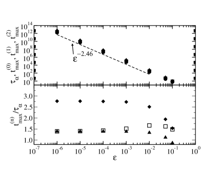
While the characteristic wave-vector is nearly constant close to the transition, the characteristic time grows rapidly as the mode-coupling transition is approached and diverges at the transition. In Fig. 2 we examine the time at which χ(n)(kmax;t)superscript𝜒𝑛subscript𝑘max𝑡\chi^{(n)}(k_{\mathrm{max}};t) is a maximum, tmax(n)superscriptsubscript𝑡max𝑛t_{\mathrm{max}}^{(n)}, as a function of ϵitalic-ϵ\epsilon for the characteristic wave-vector kmax=7.1subscript𝑘max7.1k_{\mathrm{max}}=7.1. We compare tmax(n)superscriptsubscript𝑡max𝑛t_{\mathrm{max}}^{(n)} with the α𝛼\alpha relaxation time ταsubscript𝜏𝛼\tau_{\alpha}, for which we use the standard definition F(kmax;τα)=e1𝐹subscript𝑘maxsubscript𝜏𝛼superscript𝑒1F(k_{\mathrm{max}};\tau_{\alpha})=e^{-1}. We find that tmax(n)superscriptsubscript𝑡max𝑛t_{\mathrm{max}}^{(n)} is slightly larger than ταsubscript𝜏𝛼\tau_{\alpha}, but has the same ϵitalic-ϵ\epsilon dependence, i.e. tmax(n)ϵ2.46similar-tosuperscriptsubscript𝑡max𝑛superscriptitalic-ϵ2.46t_{\mathrm{max}}^{(n)}\sim\epsilon^{2.46}. Shown in the Fig. 2b are the ratios tmax(n)/ταsuperscriptsubscript𝑡max𝑛subscript𝜏𝛼t_{\mathrm{max}}^{(n)}/\tau_{\alpha}, and it can be seen that these ratios are constant close to the mode-coupling transition. Thus, in the ϵ0italic-ϵ0\epsilon\to 0 limit we see that tmax(0)=1.4ταsuperscriptsubscript𝑡max01.4subscript𝜏𝛼t_{\mathrm{max}}^{(0)}=1.4\tau_{\alpha}, tmax(1)=2.8ταsuperscriptsubscript𝑡max12.8subscript𝜏𝛼t_{\mathrm{max}}^{(1)}=2.8\tau_{\alpha}, and tmax(2)=1.4ταsuperscriptsubscript𝑡max21.4subscript𝜏𝛼t_{\mathrm{max}}^{(2)}=1.4\tau_{\alpha}. Notice that the peak of χ(0)(kmax;t)superscript𝜒0subscript𝑘max𝑡\chi^{(0)}(k_{\mathrm{max}};t) and χ(2)(kmax;t)superscript𝜒2subscript𝑘max𝑡\chi^{(2)}(k_{\mathrm{max}};t) occur at the same time.

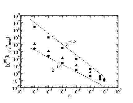
Finally, in Fig. 3 we compare the values of χ(n)(kmax;t)superscript𝜒𝑛subscript𝑘max𝑡\chi^{(n)}(k_{\mathrm{max}};t) at tmax(n)superscriptsubscript𝑡max𝑛t_{\mathrm{max}}^{(n)}. We find that |χ(0)(kmax;tmax(0))|superscript𝜒0subscript𝑘maxsuperscriptsubscript𝑡max0|\chi^{(0)}(k_{\mathrm{max}};t_{\mathrm{max}}^{(0)})| and |χ(1)(kmax;tmax(1))|superscript𝜒1subscript𝑘maxsuperscriptsubscript𝑡max1|\chi^{(1)}(k_{\mathrm{max}};t_{\mathrm{max}}^{(1)})| grow as ϵ1superscriptitalic-ϵ1\epsilon^{-1} whereas |χ(2)(kmax;tmax(2))|superscript𝜒2subscript𝑘maxsuperscriptsubscript𝑡max2|\chi^{(2)}(k_{\mathrm{max}};t_{\mathrm{max}}^{(2)})| grows as ϵ3/2superscriptitalic-ϵ32\epsilon^{-3/2}. As we discuss in the next section, this disparate behavior of χ(n)(kmax;t)superscript𝜒𝑛subscript𝑘max𝑡\chi^{(n)}(k_{\mathrm{max}};t) is important for the existence of a diverging characteristic length.

We should note at this point that the ϵitalic-ϵ\epsilon dependence of χ(n)(k;t)superscript𝜒𝑛𝑘𝑡\chi^{(n)}(k;t) can be deduced from scaling predictions described in Ref. Biroli et al. (2006), and the numerical results presented here fully agree with the these predictions.

VI Diverging characteristic length

To obtain a growing characteristic length scale as the mode-coupling transition is approached, we need |χ(n)(k;t)|superscript𝜒𝑛𝑘𝑡|\chi^{(n)}(k;t)| for some n>0𝑛0n>0 to grow faster than |χ(0)(k;t)|superscript𝜒0𝑘𝑡|\chi^{(0)}(k;t)| at a fixed time t𝑡t. Then a diverging length can be calculated as |χ(n)(k;t)/χ(0)(k;t)|(1/n)superscriptsuperscript𝜒𝑛𝑘𝑡superscript𝜒0𝑘𝑡1𝑛|\chi^{(n)}(k;t)/\chi^{(0)}(k;t)|^{(1/n)}.

From Fig. 3 it is clear that the linear term, χ(1)(k;t)superscript𝜒1𝑘𝑡\chi^{(1)}(k;t), does not result in a growing length scale. On the other hand, the absolute value of the isotropic second order term, |χ(2)(k;t)|superscript𝜒2𝑘𝑡|\chi^{(2)}(k;t)|, grows faster than χ(0)(k;t)superscript𝜒0𝑘𝑡\chi^{(0)}(k;t) and thus we can define a diverging characteristic length ξ(k;t)𝜉𝑘𝑡\xi(k;t),

ξ(k;t)=χ(2)(k;t)χ(0)(k;t),𝜉𝑘𝑡superscript𝜒2𝑘𝑡superscript𝜒0𝑘𝑡\xi(k;t)=\sqrt{-\frac{\chi^{(2)}(k;t)}{\chi^{(0)}(k;t)}}, (38)

where the negative sign comes from the observation that χ(2)(k;t)superscript𝜒2𝑘𝑡\chi^{(2)}(k;t) is of opposite sign of χ(0)(k;t)superscript𝜒0𝑘𝑡\chi^{(0)}(k;t) around ταsubscript𝜏𝛼\tau_{\alpha} and close to the transition. Note that for large times t𝑡t, Eq. 38 involves a division of a small number by another small number. Because of numerical issues present in the algorithm to calculate χ(n)(k;t)superscript𝜒𝑛𝑘𝑡\chi^{(n)}(k;t), we only show results if χ(n)(k;t)103superscript𝜒𝑛𝑘𝑡superscript103\chi^{(n)}(k;t)\geq 10^{-3}, and therefore we, unfortunately, cannot comment at the asymptotic t𝑡t\to\infty limit of the characteristic length.

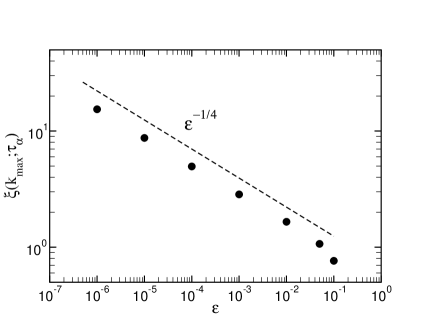
In Fig. 4 we examine ξ(kmax;τα)𝜉subscript𝑘maxsubscript𝜏𝛼\xi(k_{\mathrm{max}};\tau_{\alpha}), i.e. the characteristic length at k=kmax𝑘subscript𝑘maxk=k_{\mathrm{max}} and at the α𝛼\alpha relaxation time. The length ξ(kmax;τα)𝜉subscript𝑘maxsubscript𝜏𝛼\xi(k_{\mathrm{max}};\tau_{\alpha}) grows as ϵ1/4superscriptitalic-ϵ14\epsilon^{-1/4} and it reaches only 15 particle diameters at ϵ=106italic-ϵsuperscript106\epsilon=10^{-6}. Thus the characteristic length is not very large even very close to the transition. For ϵ=0.05italic-ϵ0.05\epsilon=0.05, we find that ξ(kmax;τα)𝜉subscript𝑘maxsubscript𝜏𝛼\xi(k_{\mathrm{max}};\tau_{\alpha}) is only about one particle diameter. Note that Eq. (38) defines a length scale for every wave-vector k𝑘k and at all times t𝑡t, and we examine the time and wave-vector dependence of ξ(k;t)𝜉𝑘𝑡\xi(k;t) below.

We determined that setting the initial condition for χ(2)(k;t=0)superscript𝜒2𝑘𝑡0\chi^{(2)}(k;t=0) to zero and/or taking 𝒮(2)(k;t)=0superscript𝒮2𝑘𝑡0\mathcal{S}^{(2)}(k;t)=0 had very little effect on the size of the correlation length close to the mode-coupling transition. While including these terms is in principle straightforward, dropping them significantly simplifies the numerical calculation.
Refer to caption
Figure 2: Upper Panel: the α𝛼\alpha relaxation time, ταsubscript𝜏𝛼\tau_{\alpha} (filled circles), and the peak positions of χ(n)(kmax;t)superscript𝜒𝑛subscript𝑘max𝑡\chi^{(n)}(k_{\mathrm{max}};t), τmax(n)superscriptsubscript𝜏max𝑛\tau_{\mathrm{max}}^{(n)}, as a function of ϵ=(ϕϕc)/ϕcitalic-ϵitalic-ϕsubscriptitalic-ϕ𝑐subscriptitalic-ϕ𝑐\epsilon=(\phi-\phi_{c})/\phi_{c}: τmax(0)subscriptsuperscript𝜏0max\tau^{(0)}_{\mathrm{max}}–triangles; τmax(1)subscriptsuperscript𝜏1max\tau^{(1)}_{\mathrm{max}}–diamonds; τmax(2)subscriptsuperscript𝜏2max\tau^{(2)}_{\mathrm{max}}–open squares. Lower Panel: the ratio τmax(n)/ταsuperscriptsubscript𝜏max𝑛subscript𝜏𝛼\tau_{\mathrm{max}}^{(n)}/\tau_{\alpha} as a function of ϵitalic-ϵ\epsilon.
Refer to caption
Figure 3: The peak height of χ(n)(k;t)superscript𝜒𝑛𝑘𝑡\chi^{(n)}(k;t) as a function of the distance from the mode coupling transition ϵitalic-ϵ\epsilon. χ(0)(kmax;tmax)superscript𝜒0subscript𝑘maxsubscript𝑡max\chi^{(0)}(k_{\mathrm{max}};t_{\mathrm{max}}) – triangles; χ(1)(kmax;tmax)superscript𝜒1subscript𝑘maxsubscript𝑡max\chi^{(1)}(k_{\mathrm{max}};t_{\mathrm{max}}) – circles; χ(2)(kmax;tmax)superscript𝜒2subscript𝑘maxsubscript𝑡max\chi^{(2)}(k_{\mathrm{max}};t_{\mathrm{max}}) – squares
Refer to caption
Figure 4: The characteristic dynamic length ξ(kmax;τα)𝜉subscript𝑘maxsubscript𝜏𝛼\xi(k_{\mathrm{max}};\tau_{\alpha}) as a function of the distance from the transition ϵitalic-ϵ\epsilon.

Fourier transforms of four-point correlation functions, i.e. four-point dynamic structure factors, are often monitored in simulations and used to investigate properties of dynamic heterogeneities. Since the q=0𝑞0q=0 value of a four-point structure factor should be proportional to the characteristic volume in which correlated motion takes place, an increase of the q=0𝑞0q=0 value (i.e. of the height of four-point structure factor) is often given as evidence of an increase in a dynamic correlation length.

Similarly, for the problem considered here, the value of χ(0)(k;t)superscript𝜒0𝑘𝑡\chi^{(0)}(k;t) could used as an indicator of the size of a characteristic dynamic range of the response. However, the spatial extent of dynamic response is best measured by examining the long-range spatial decay of a direct space susceptibility or, alternatively, by examining the small-q𝑞q behavior of the susceptibility χ𝐪(𝐤;t)subscript𝜒𝐪𝐤𝑡\chi_{\mathbf{q}}(\mathbf{k};t). This distinction is significant in view of the very strong wave-vector and time dependence of χ(0)(k;t)superscript𝜒0𝑘𝑡\chi^{(0)}(k;t). In particular, if the characteristic length were a monotonic function of χ(0)(k;t)superscript𝜒0𝑘𝑡\chi^{(0)}(k;t), then Fig. 1 would be leading to the unfortunate conclusion that ξ(k;t)𝜉𝑘𝑡\xi(k;t) is a very strong function of k𝑘k. The length would then have a rather limited appeal. In the following paragraph we show that this is not the case.

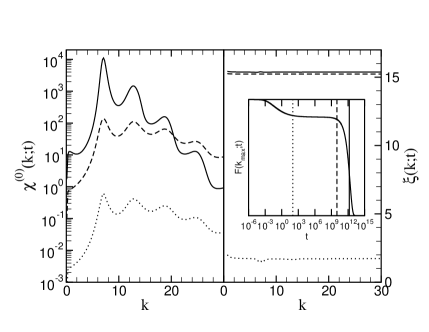
In Fig. 5 we compare the k𝑘k dependence of ξ(k;t)𝜉𝑘𝑡\xi(k;t) (right figure) and χ(0)(k;t)superscript𝜒0𝑘𝑡\chi^{(0)}(k;t) (left figure) for three characteristic times: (1) early β𝛽\beta (dotted line), late-β𝛽\beta (dashed line), and at the α𝛼\alpha relaxation time (solid line). For reference, F(kmax;t)𝐹subscript𝑘max𝑡F(k_{\mathrm{max}};t) is shown in the insert to Fig. 5 with the three characteristic times shown as vertical lines in the figure. There is a very strong dependence of χ(0)(k;t)superscript𝜒0𝑘𝑡\chi^{(0)}(k;t) on k𝑘k, but ξ(k;τα)𝜉𝑘subscript𝜏𝛼\xi(k;\tau_{\alpha}) is nearly constant at each time. Therefore, even though there is a strong k𝑘k dependence of the three-point susceptibility, there is a well defined characteristic dynamic length ξ(k;t)𝜉𝑘𝑡\xi(k;t) that is independent of k𝑘k and only depends on the time t𝑡t. This suggests that we could drop the explicit k𝑘k dependence of ξ(k;t)𝜉𝑘𝑡\xi(k;t) and introduce a simplified notation ξ(t)𝜉𝑡\xi(t).

Refer to caption
Figure 5: Left panel: the wave-vector dependence of the 𝐪=0𝐪0\mathbf{q}=0 value of the three-point susceptibility, χ𝐪=0(𝐤;t)χ(0)(k;t)subscript𝜒𝐪0𝐤𝑡superscript𝜒0𝑘𝑡\chi_{\mathbf{q}=0}(\mathbf{k};t)\equiv\chi^{(0)}(k;t), at a time corresponding the the early β𝛽\beta relaxation regime (dotted line), the late β𝛽\beta regime (dashed line), and the α𝛼\alpha relaxation time (solid line). Right panel: the wave-vector dependence of the characteristic dynamic length ξ(k;t)𝜉𝑘𝑡\xi(k;t) for the same times as in the left panel. The inset is the self-intermediate scattering function F(k;t)𝐹𝑘𝑡F(k;t) and the three vertical lines correspond to the three times in left and right panels.

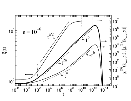
Next, we investigate the time dependence of the characteristic length. Shown in Fig. 6 is χ(0)(kmax;t)superscript𝜒0subscript𝑘max𝑡\chi^{(0)}(k_{\mathrm{max}};t) (lower curve-right axis), |χ(2)(kmax;t)|superscript𝜒2subscript𝑘max𝑡|\chi^{(2)}(k_{\mathrm{max}};t)| (middle curve-right axis), and ξ(t)𝜉𝑡\xi(t) (upper curve-left axis) as a function of time for ϵ=106italic-ϵsuperscript106\epsilon=10^{-6}. The correlation length ξ(t)𝜉𝑡\xi(t) is close to one for t=0𝑡0t=0, begins to grow during β𝛽\beta relaxation and reaches a plateau at a time corresponding to the late β𝛽\beta-early α𝛼\alpha relaxation. During the α𝛼\alpha relaxation, ξ(t)𝜉𝑡\xi(t) is approximately constant. Note that ξ(t)𝜉𝑡\xi(t) has a very different time dependence than χ(0)(kmax;t)superscript𝜒0subscript𝑘max𝑡\chi^{(0)}(k_{\mathrm{max}};t). Therefore, the length scale associated with dynamic heterogeneities are not a maximum when χ(0)(k;t)superscript𝜒0𝑘𝑡\chi^{(0)}(k;t) is a maximum, but rather reaches a constant value for times less than this characteristic time.
Refer to caption
Figure 6: The time dependence of the characteristic dynamic length ξ(t)𝜉𝑡\xi(t) (left solid line and left axis), the susceptibility χ(0)(kmax;t)superscript𝜒0subscript𝑘max𝑡\chi^{(0)}(k_{\mathrm{max}};t) (right solid line and right axis), and the second order coefficient χ(2)(kmax;t)superscript𝜒2subscript𝑘max𝑡\chi^{(2)}(k_{\mathrm{max}};t) (middle, heavy solid line and right axis), showed on a log-log scale. The dashed lines show the scaling laws in the β𝛽\beta relaxation regime. The vertical lines crossing ξ(t)𝜉𝑡\xi(t) correspond to the three times shown in the inset to Fig. 5.

Scaling relations for different time regimes can be derived from the predictions of the mode coupling theory Biroli et al. (2006); Berthier et al. (2007). Specifically, in the early β𝛽\beta regime χ(0)(k;t)tasimilar-tosuperscript𝜒0𝑘𝑡superscript𝑡𝑎\chi^{(0)}(k;t)\sim t^{a}, and in the late β𝛽\beta regime χ(0)(k;t)tbsimilar-tosuperscript𝜒0𝑘𝑡superscript𝑡𝑏\chi^{(0)}(k;t)\sim t^{b} where a=0.312𝑎0.312a=0.312 and b=0.583𝑏0.583b=0.583 for our system. The power law growth of χ(0)(t)superscript𝜒0𝑡\chi^{(0)}(t) and χ(2)(t)superscript𝜒2𝑡\chi^{(2)}(t) are also shown in Fig. 6. During the early β𝛽\beta relaxation regime, χ(0)(t)tasimilar-tosuperscript𝜒0𝑡superscript𝑡𝑎\chi^{(0)}(t)\sim t^{a} while χ(2)(t)t2asimilar-tosuperscript𝜒2𝑡superscript𝑡2𝑎\chi^{(2)}(t)\sim t^{2a}, which gives rise to the ta/2superscript𝑡𝑎2t^{a/2} growth of the correlation length in the early β𝛽\beta relaxation regime. However, during late β𝛽\beta relaxation, χ(2)(t)superscript𝜒2𝑡\chi^{(2)}(t) and χ(0)(t)superscript𝜒0𝑡\chi^{(0)}(t) both grow as tbsuperscript𝑡𝑏t^{b}, thus there is no growing length scale. The vertical lines in the figure denote the same times as the vertical lines in the inset to Fig. 5.

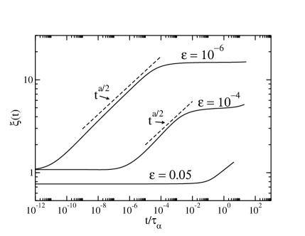
In Fig. 7 we show ξ(kmax;t)𝜉subscript𝑘max𝑡\xi(k_{\mathrm{max}};t) as a function of t/τα𝑡subscript𝜏𝛼t/\tau_{\alpha} for ϵ=0.05italic-ϵ0.05\epsilon=0.05, 104superscript10410^{-4}, and 106superscript10610^{-6}. For ϵ=104italic-ϵsuperscript104\epsilon=10^{-4} we observe the ta/2superscript𝑡𝑎2t^{a/2} scaling for only a very narrow range of time, and we do not observe the ta/2superscript𝑡𝑎2t^{a/2} scaling for any time range at ϵ=0.05italic-ϵ0.05\epsilon=0.05, which suggests that it might be very difficult to see this scaling in simulations.
Refer to caption
Figure 7: The characteristic dynamic length ξ(kmax;t)𝜉subscript𝑘max𝑡\xi(k_{\mathrm{max}};t) as a function of t/τα𝑡subscript𝜏𝛼t/\tau_{\alpha} for ϵ=0.05italic-ϵ0.05\epsilon=0.05, 104superscript10410^{-4} and 106superscript10610^{-6}. The dashed lines is the scaling law ξ(t)ta/2similar-to𝜉𝑡superscript𝑡𝑎2\xi(t)\sim t^{a/2} valid in the β𝛽\beta relaxation regime.

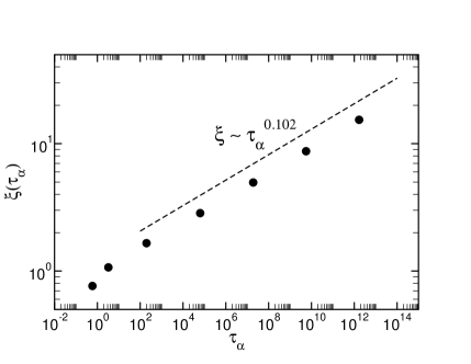
Finally, we note that since ταϵ2.46similar-tosubscript𝜏𝛼superscriptitalic-ϵ2.46\tau_{\alpha}\sim\epsilon^{-2.46} and ξϵ0.25similar-to𝜉superscriptitalic-ϵ0.25\xi\sim\epsilon^{-0.25}, then ξτα0.102similar-to𝜉superscriptsubscript𝜏𝛼0.102\xi\sim\tau_{\alpha}^{0.102}, Fig. 8. As a result, a modest increase in the correlation length is accompanied by a very large increase of the relaxation time.
Refer to caption
Figure 8: The characteristic dynamic length ξ(τα)𝜉subscript𝜏𝛼\xi(\tau_{\alpha}) calculated at the α𝛼\alpha relaxation time as a function of the α𝛼\alpha relaxation time.

VII Numerical evaluation of χqiso(k;t)superscriptsubscript𝜒𝑞iso𝑘𝑡\chi_{q}^{\mathrm{iso}}(k;t) and associated characteristic length

The isotropic approximation neglects the dependence of the three-point susceptibility on the angle between 𝐤𝐤\mathbf{k} and 𝐪𝐪\mathbf{q}. Thus, in the resulting equation of motion for χqiso(k;t)superscriptsubscript𝜒𝑞iso𝑘𝑡\chi_{q}^{\mathrm{iso}}(k;t) q𝑞q is just a parameter, and the equation of motion can be solved separately for any value of q𝑞q. As a result, the full q𝑞q dependence of χqiso(k;t)superscriptsubscript𝜒𝑞iso𝑘𝑡\chi_{q}^{\mathrm{iso}}(k;t) can be calculated. On the other hand, the isotropic approximation preserves the essential terms in the equation of motion which lead to the divergence of the q0𝑞0q\to 0 limit of χqiso(k;t)superscriptsubscript𝜒𝑞iso𝑘𝑡\chi_{q}^{\mathrm{iso}}(k;t) and of the characteristic length. In this section we examine the isotropic approximation and compare this approximation to the expansion terms given above. Since the equations of motion are similar and the terms that cause the divergence are identical, many of the results of Sec. V carry over to the isotropic approximation. Notably, as we already noted in Sec. IV, χ(0)(k;t)superscript𝜒0𝑘𝑡\chi^{(0)}(k;t) is identical in both cases.

Since we can calculate the whole q𝑞q dependence in the isotropic approximation, we can determine the characteristic length ξ(t)𝜉𝑡\xi(t) using two different methods. We can either evaluate χqiso(k;t)superscriptsubscript𝜒𝑞iso𝑘𝑡\chi_{q}^{\mathrm{iso}}(k;t) and then fit χqiso(k;t)/χ(0)(k;t)superscriptsubscript𝜒𝑞iso𝑘𝑡superscript𝜒0𝑘𝑡\chi_{q}^{\mathrm{iso}}(k;t)/\chi^{(0)}(k;t) to 1(ξiso(k;t)q)21superscriptsuperscript𝜉iso𝑘𝑡𝑞21-(\xi^{\mathrm{iso}}(k;t)q)^{2} for small q𝑞q or we can determine ξiso(k;t)superscript𝜉iso𝑘𝑡\xi^{\mathrm{iso}}(k;t) from χiso(2)(k;t)/χ(0)(k;t)superscript𝜒𝑖𝑠𝑜2𝑘𝑡superscript𝜒0𝑘𝑡\sqrt{-\chi^{iso(2)}(k;t)/\chi^{(0)}(k;t)}. Both methods result in the same length.

It can be showed that within the isotropic approximation the characteristic length is almost k𝑘k-independent (and thus we will denote it by ξiso(t)superscript𝜉iso𝑡\xi^{\mathrm{iso}}(t)). In addition, the time dependence of the length is very similar to what was obtained from the full equations of motion in Sec. V.

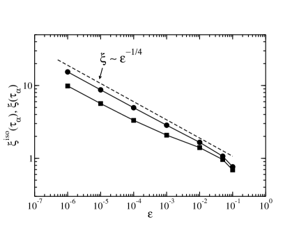
In Fig. 9 we compare the magnitude of the characteristic length obtained from the isotropic approximation, ξiso(τα)superscript𝜉isosubscript𝜏𝛼\xi^{\mathrm{iso}}(\tau_{\alpha}), with that following from the full equations of motion, ξ(τα)𝜉subscript𝜏𝛼\xi(\tau_{\alpha}). As we anticipated in the first paragraph of this section, the isotropic approximation gives a length which diverges as ϵ1/4superscriptitalic-ϵ14\epsilon^{-1/4}. However, the isotropic approximation underestimates the characteristic length; for small ϵitalic-ϵ\epsilon the length resulting from the isotropic approximation is approximately 36% smaller than the length resulting from the expansion of the complete equation (4).
Refer to caption
Figure 9: The characteristic dynamic length ξiso(k;t)superscript𝜉iso𝑘𝑡\xi^{\mathrm{iso}}(k;t) calculated using the isotropic approximation (squares) and without the isotropic approximation (circles).

There has been some discussion in the literature as to what scaling function should be used to determine ξ(t)𝜉𝑡\xi(t). According to the scaling relation presented in Ref. Biroli et al. (2006), in the β𝛽\beta and α𝛼\alpha regimes the divergent part of χ𝐪(𝐤;t)subscript𝜒𝐪𝐤𝑡\chi_{\mathbf{q}}(\mathbf{k};t) is a function of a scaling variable qξ(t)𝑞𝜉𝑡q\xi(t) only for small q𝑞q close to the transition, χ𝐪(𝐤;t)=𝒳β,α(qξ(tβ,α),k)subscript𝜒𝐪𝐤𝑡subscript𝒳𝛽𝛼𝑞𝜉subscript𝑡𝛽𝛼𝑘\chi_{\mathbf{q}}(\mathbf{k};t)=\mathcal{X}_{\beta,\alpha}(q\xi(t_{\beta,\alpha}),k). We use the isotropic approximation to examine some properties of scaling function 𝒳β,αsubscript𝒳𝛽𝛼\mathcal{X}_{\beta,\alpha} close to the mode coupling transition, in the β𝛽\beta and α𝛼\alpha regimes.

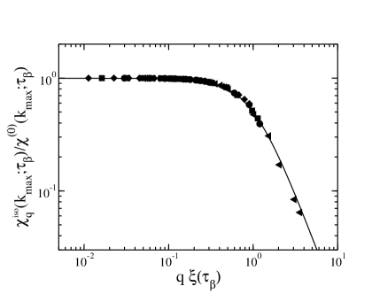
For times t𝑡t in the vicinity of the β𝛽\beta relaxation time τβsubscript𝜏𝛽\tau_{\beta}, the scaling function 𝒳β(qξ(tβ),k)subscript𝒳𝛽𝑞𝜉subscript𝑡𝛽𝑘\mathcal{X}_{\beta}(q\xi(t_{\beta}),k) is predicted to have the Ornstein-Zernicke behavior, namely 𝒳β(qξ(tβ),k)subscript𝒳𝛽𝑞𝜉subscript𝑡𝛽𝑘\mathcal{X}_{\beta}(q\xi(t_{\beta}),k) should scale as q2superscript𝑞2q^{-2} for large q𝑞q Biroli et al. (2006). To check this prediction we first need to define the β𝛽\beta relaxation time. We define τβsubscript𝜏𝛽\tau_{\beta} as the inflection point of F(t)𝐹𝑡F(t) versus ln(t)𝑡\ln(t). We verified that this definition agrees with the MCT scaling τβϵ1/2asimilar-tosubscript𝜏𝛽superscriptitalic-ϵ12𝑎\tau_{\beta}\sim\epsilon^{-1/2a}. This time τβsubscript𝜏𝛽\tau_{\beta} is only well defined for ϵ103italic-ϵsuperscript103\epsilon\leq 10^{-3}. Shown in Fig. 10 is χqiso(kmax;τβ)/χ(0)(kmax;τβ)superscriptsubscript𝜒𝑞isosubscript𝑘maxsubscript𝜏𝛽superscript𝜒0subscript𝑘maxsubscript𝜏𝛽\chi_{q}^{\mathrm{iso}}(k_{\mathrm{max}};\tau_{\beta})/\chi^{(0)}(k_{\mathrm{max}};\tau_{\beta}) as a function of qξ(τα)𝑞𝜉subscript𝜏𝛼q\xi(\tau_{\alpha}) and the Ornstein-Zernicke function 1/[1+(ξq)2]1delimited-[]1superscript𝜉𝑞21/[1+(\xi q)^{2}], which provides a good fit for small q𝑞q during the β𝛽\beta relaxation time and demonstrates the q2superscript𝑞2q^{-2} scaling for large q𝑞q.

Refer to caption
Figure 10: The isotropic approximation for the dynamic susceptibility χqiso(kmax;τβ)superscriptsubscript𝜒𝑞isosubscript𝑘maxsubscript𝜏𝛽\chi_{q}^{\mathrm{iso}}(k_{\mathrm{max}};\tau_{\beta}) as a function of qξ(τβ)𝑞𝜉subscript𝜏𝛽q\xi(\tau_{\beta}) for ϵ103italic-ϵsuperscript103\epsilon\leq 10^{-3}. Only data for q𝑞q in the scaling regime are included. The solid line is the Ornstein-Zernicke function 1/[1+(ξq)2]1delimited-[]1superscript𝜉𝑞21/[1+(\xi q)^{2}].

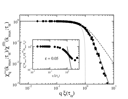
For times t𝑡t comparable to the α𝛼\alpha relaxation time ταsubscript𝜏𝛼\tau_{\alpha}, the inhomogeneous mode-coupling theory Biroli et al. (2006) predicts a q4superscript𝑞4q^{-4} behavior of the scaling function 𝒳α(qξ(tα),k)subscript𝒳𝛼𝑞𝜉subscript𝑡𝛼𝑘\mathcal{X}_{\alpha}(q\xi(t_{\alpha}),k)at large q𝑞q. We test this prediction in Fig. 11: we show χqiso(kmax;τα)/χ(0)(kmax;τα)superscriptsubscript𝜒𝑞isosubscript𝑘maxsubscript𝜏𝛼superscript𝜒0subscript𝑘maxsubscript𝜏𝛼\chi_{q}^{\mathrm{iso}}(k_{\mathrm{max}};\tau_{\alpha})/\chi^{(0)}(k_{\mathrm{max}};\tau_{\alpha}) as a function of qξ(τα)𝑞𝜉subscript𝜏𝛼q\xi(\tau_{\alpha}) along with two functions commonly used to find ξ(t)𝜉𝑡\xi(t) in simulations, and a function suggested by the inhomogeneous mode-coupling theory. The functions 1(ξq)21superscript𝜉𝑞21-(\xi q)^{2} (dotted line) and the Ornstein-Zernicke function, 1/(1+[ξq]2)11superscriptdelimited-[]𝜉𝑞21/(1+[\xi q]^{2}), (dashed line) are good fits only to a very narrow q𝑞q range, with the Ornstein-Zernicke function being a better fit for a larger range of q𝑞q values. On the other hand, the function 1/[1+(ξq)2+a(ξq)4]1delimited-[]1superscript𝜉𝑞2𝑎superscript𝜉𝑞41/[1+(\xi q)^{2}+a(\xi q)^{4}] where a=0.45𝑎0.45a=0.45 (solid line), provides a good fit over a large q𝑞q range and thus it confirms the q4superscript𝑞4q^{-4} scaling predicted by the inhomogeneous mode-coupling theory for the α𝛼\alpha relaxation time scale. Note that the q4superscript𝑞4q^{-4} scaling is not evident for ϵ=0.05italic-ϵ0.05\epsilon=0.05 (inset), which suggests that this scaling might be difficult to observe in simulations.
Refer to caption
Figure 11: The isotropic approximation for the dynamic susceptibility χqiso(kmax;τα)superscriptsubscript𝜒𝑞isosubscript𝑘maxsubscript𝜏𝛼\chi_{q}^{\mathrm{iso}}(k_{\mathrm{max}};\tau_{\alpha}) as a function of qξ(τα)𝑞𝜉subscript𝜏𝛼q\xi(\tau_{\alpha}) for ϵ103italic-ϵsuperscript103\epsilon\leq 10^{-3}. Only data for q𝑞q in the scaling regime are included. The dotted line is 1(qξ)21superscript𝑞𝜉21-(q\xi)^{2}, the dashed line is 1/[1+(qξ)2]1delimited-[]1superscript𝑞𝜉21/[1+(q\xi)^{2}]. The solid line is a fit to the data to a function of the form 1/[1+(qξ)2+a(qξ)4]1delimited-[]1superscript𝑞𝜉2𝑎superscript𝑞𝜉41/[1+(q\xi)^{2}+a(q\xi)^{4}] where a=0.45𝑎0.45a=0.45. The q4superscript𝑞4q^{-4} scaling for large q𝑞q is evident. Inset: the dynamic susceptibility χqiso(kmax;τα)superscriptsubscript𝜒𝑞isosubscript𝑘maxsubscript𝜏𝛼\chi_{q}^{\mathrm{iso}}(k_{\mathrm{max}};\tau_{\alpha}) for ϵ=0.05italic-ϵ0.05\epsilon=0.05 showing all the data including q𝑞q values beyond the scaling regime. The inset shows that the q4superscript𝑞4q^{-4} scaling (solid line) is not apparent for this ϵitalic-ϵ\epsilon.

VIII Conclusions

We used inhomogeneous mode-coupling theory to numerically investigate the dynamic susceptibility χ𝐪(𝐤;t)subscript𝜒𝐪𝐤𝑡\chi_{\mathbf{q}}(\mathbf{k};t) at small q𝑞q and determined time, k𝑘k, and distance from the transition dependence of the diverging characteristic length scale. We confirmed scaling predictions presented in Ref. Biroli et al. (2006) and obtained a couple of new interesting results. Because of numerical issues, we were not able to calculate the asymptotic long time behavior of the diverging characteristic length scale. This would be an interesting topic that we leave for later analysis. It most likely requires an analytical argument that goes beyond the scaling analysis presented in Ref. Biroli et al. (2006).

The most important result of our numerical investigation is that the diverging characteristic length is very weakly k𝑘k dependent. This makes it a well defined quantity. We speculate that the k𝑘k independence of the characteristic length should carry over to the dynamic correlation length defined in terms of a four-point structure factor. Moreover, it should explain why a variety of slightly different four point functions (e.g. defined in terms of overlap functions Lacevic et al. (2003); Stein and Andersen (2008); Karamakar et al. (2009) or in terms of self-intermediate scattering functions Berthier (2004); Toninelli et al. (2005); Flenner and Szamel (2009)) result in comparable dynamic correlation lengths.

The second important result, which cannot be obtained from scaling considerations alone, is the magnitude of the characteristic length. On general grounds we expect this length to be comparable to dynamic correlation lengths defined through four-point structure factors. Thus, it is satisfying that the magnitude of the length is indeed comparable (albeit somewhat smaller) to what’s found in simulations.

We would like to point out that, although various simulations found comparable values of the dynamic correlation length, there are a few important unresolved differences between results obtained by different groups that preclude declaring that the characteristic length discussed in this work is essentially the same as the dynamic correlation length measured in simulations.

First, while the characteristic length defined through the three-point susceptibility is a monotonic function of time (at least as long as our numerical routines are reliable), the simulational results very. Lacevic et al. Lacevic et al. (2003) found that the dynamic correlation length roughly followed the overall magnitude of the four-point correlation function and decayed to zero at later times. In contrast, Toninelli et al. Toninelli et al. (2005) found that the dynamic correlation length continued to grow at later times. While slightly different fitting procedures were used in these two works, it is difficult to pinpoint the exact source of two strikingly different results.

Second, within the mode-coupling approximation, the characteristic length defined through the three-point susceptibility diverges as ϵ1/4superscriptitalic-ϵ14\epsilon^{-1/4} upon approaching the ergodicity breaking transition predicted by the mode-coupling theory. We feel that the relevance of this result to simulations (and experiments) in which the mode-coupling transtion is avoided still needs to be fully established. We speculate that it is possible that in computer simulations a vestige of a power law divergence of the dynamic correlation length could be seen just as one can observe in simulations power law dependencies of various transport coefficients upon approaching a mode-coupling crossover Flenner and Szamel (2005). Indeed, various groups have already claimed power law dependencies of their dynamic correlation lengths upon approaching the mode-coupling crossover (see, e.g. Berthier (2004); Whitelam et al. (2004); Flenner and Szamel (2009); Stein and Andersen (2008); Karamakar et al. (2009)). However, there seems to be some disagreement regarding the value of the scaling exponent and only one work, Stein and Andersen (2008), results in a value agreeing with the prediction of the inhomogeneous mode-coupling theory. Upon closer examination of the fitting procedure described in Ref. Stein (2007) and re-examining our own simulation data we concluded that virtually all systems studied in simulations were not large enough to obtain the dynamic correlation length in a range allowing for an unambiguous determination of the scaling exponent.

IX Acknowledgment

We would like to thank G. Biroli, K. Miyazaki and D. Reichman for comments about this work. We gratefully acknowledge the support of NSF Grant No. CHE 0517709.

References

  • Ediger (2000) M. Ediger, Annu. Rev. Phys. Chem. 51, 99 (2000).
  • Richert (2002) R. Richert, J. Phys.: Condens. Matter 14, R703 (2002).
  • Andersen (2005) H. Andersen, Proc. Natl. Acad. Sci. U.S.A. 102, 6686 (2005).
  • Lacevic et al. (2002) N. Lacevic, F. Starr, T. Schroder, V. Novikov, and S. Glotzer, Phys. Rev. E 66, 030101(R) (2002).
  • Lacevic et al. (2003) N. Lacevic, F. Starr, T. Schroder, and S. Glotzer, J. Chem. Phys. 119, 7372 (2003).
  • Berthier (2004) L. Berthier, Phys. Rev. E 69, 020201(R) (2004).
  • Toninelli et al. (2005) C. Toninelli, M. Wyart, L. Berthier, G. Biroli, and J. Bouchaud, Phys. Rev. E 71, 041505 (2005).
  • Berthier et al. (2007) L. Berthier, G. Biroli, J. Bouchaud, W. Kob, K. Miyazaki, and D. Reichman, J. Chem. Phys. 126, 184503 (2007).
  • Lechenault et al. (2008a) F. Lechenault, O. Dauchot, G. Biroli, and J. Bouchaud, Europhys. Lett. 83, 46002 (2008a).
  • Lechenault et al. (2008b) F. Lechenault, O. Dauchot, G. Biroli, and J. Bouchaud, Europhys. Lett. 83, 46003 (2008b).
  • Berthier et al. (2005) L. Berthier, G. Biroli, J. Bouchaud, L. Cipelletti, D. Masri, D. L’Hote, F. Ladieu, and M. Pierno, Science 310, 1797 (2005).
  • Dalle-Ferrier et al. (2007) C. Dalle-Ferrier, C. Thibierge, C. Alba-Simionesco, L. Berthier, G. Biroli, J. Bouchaud, F. Ladieu, D. L’Hote, and G. Tarjus, Phys. Rev. E 76, 041510 (2007).
  • Biroli et al. (2006) G. Biroli, J. Bouchaud, K. Miyazaki, and D. Reichman, Phys. Rev. Lett. 97, 195701 (2006).
  • (14) G. Szamel, unpublished.
  • Fuchs et al. (1991) M. Fuchs, W. Gotze, I. Hofacker, and A. Latz, J. Phys.: Condens. Matter 3, 5047 (1991).
  • (16) K. Miyazaki, B. Bagchi, and Yethiraj, cond-mat/0405326v1. Note that the published version of this manuscript [J. Chem. Phys. 121, 8120 (2004)] does not contain the detailed description of the numerical algorithm.
  • Flenner and Szamel (2005) E. Flenner and G. Szamel, Phys. Rev. E 72, 031508 (2005).
  • Szamel and Flenner (2009) G. Szamel and E. Flenner, Phys. Rev. E 79, 021503 (2009).
  • Stein and Andersen (2008) R. Stein and H. Andersen, Phys. Rev. Lett. 101, 267802 (2008).
  • Karamakar et al. (2009) S. Karamakar, C. Dasgupta, and S. Sastry, PNAS 106, 3675 (2009).
  • Flenner and Szamel (2009) E. Flenner and G. Szamel, Phys. Rev. E 79, 051502 (2009).
  • Whitelam et al. (2004) S. Whitelam, L. Berthier, and J. Garrahan, Phys. Rev. Lett. 92, 185705 (2004).
  • Stein (2007) R. Stein, Ph.D. thesis, Stanford University (2007).