A variational principle
for computing slow invariant manifolds
in dissipative dynamical systems

Abstract

A key issue in dimension reduction of dissipative dynamical systems with spectral gaps is the identification of slow invariant manifolds. We present theoretical and numerical results for a variational approach to the problem of computing such manifolds for kinetic models using trajectory optimization. The corresponding objective functional reflects a variational principle that characterizes trajectories on, respectively near, slow invariant manifolds. For a two-dimensional linear system and a common nonlinear test problem we show analytically that the variational approach asymptotically identifies the exact slow invariant manifold in the limit of both an infinite time horizon of the variational problem with fixed spectral gap and infinite spectral gap with a fixed finite time horizon. Numerical results for the linear and nonlinear model problems as well as a more realistic higher-dimensional chemical reaction mechanism are presented.

1 Introduction

In dissipative ordinary differential equation systems modeling chemical reaction kinetics the phase flow generally causes anisotropic volume contraction due to multiple time scales with spectral gaps. This leads to a bundling of trajectories near “invariant manifolds of slow motion” of successively lower dimension during time evolution. Model reduction methods exploit this for simplifying the underlying ordinary differential equation models via time scale separation into fast and slow modes and eliminating the fast modes by enslaving them to the slow ones as a graph of a function which defines the slow invariant (attracting) manifold (SIM).

Early model reduction approaches in chemical kinetics like the quasi steady-state and partial equilibrium assumption [32] have been performed “by hand”, modern numerical approaches are supposed to automatically compute a reduced model without need for detailed expert knowledge of chemical kinetics by the user. Many of these techniques are based on an explicit time-scale analysis of the underlying ordinary differential equation (ODE) system.

Among those methods that became popular in applications are the intrinsic low dimensional manifold (ILDM) method [21] and recent extensions of its main ideas, e.g. the global quasi-linearization (GQL) [4], computational singular perturbation (CSP) [15, 16], Fraser’s algorithm [6, 9, 23], the method of invariant grids [5, 11, 12], the constrained runs algorithm [10, 33], rate-controlled constrained equilibrium (RCCE) [14], the invariant constrained equilibrium edge preimage curve (ICE-PIC) method [27, 28], flamelet-generated manifolds [7, 30], and finite time Lyapunov exponents [22]. For a comprehensive overview see e.g. [11] and references therein.

Reaction trajectories in phase space that are solutions of an ODE system $\dot{x}(t)=f(x(t)),x(0)=x_{0},f\in C^{\infty}$, describing chemical kinetics are uniquely determined by their initial values and the corresponding orbits bear global information about phase space structure. Based on Lebiedz’ idea to search for an extremum principle that distinguishes trajectories on or near slow attracting manifolds, an optimization approach for computing such trajectories has been applied in [17, 18, 26]. In [19] the authors propose and discuss various geometrically motivated optimization criteria for the formulation of a suitable extremum principle and present numerical results for several applications.

The present work systematically analyzes a variational formulation of the problem to compute slow invariant manifolds and its potential for identifying the correct manifold for linear and nonlinear test problems in two-dimensional phase space. We analytically prove the correct identification of the slow eigenspace and SIM respectively in the limit of infinite-time horizon of the variational problem and derive an error quantification as a function of spectral gap and finite time horizon length. In addition, we provide corresponding numerical results confirming the theoretical prediction.

2 Variational Problem

We consider autonomous ODE systems of the form $\dot{x}=f(x)$ modeling chemical reaction kinetics that have a stable fixed point corresponding to chemical equilibrium. The basic idea of our approach is the formulation of a variational principle that captures essential properties of a slow invariant manifold (SIM). We propose an appropriate characterization of maximum “slowness” in terms of an integral over suitably defined curvature (velocity change) of trajectories measured in the Euclidean norm. The SIM is generally characterized by the property that all trajectories in its neighborhood converge faster to the manifold than to the attractor, the chemical equilibrium point. Adrover et al. [1] recently argued that this might be interpreted as a ratio $r>1$ of the local stretching (contraction) rate of vectors orthogonal to the manifold compared to those tangent to the manifold. This point of view comes close to our reasoning on the basis of a variational principle.

2.1 Trajectory-Based Optimization Approach

The variational problem can be formulated as

$$\min_{x(t)}\int_{t_{0}}^{t_{\mathrm{f}}}\Phi\left(x(t)\right)\;\mathrm{d}t$$ (1a)

subject to

$$\frac{\mathrm{d}x(t)}{\mathrm{d}t} =f\left(x(t)\right)$$ (1b)

$$0 =g\left(x(t_{*})\right)$$ (1c)

$$x_{j}(t_{*}) =x_{j}^{t_{*}},\quad j\in I_{\text{fixed}},$$ (1d)

with $t_{0}\leqslant t_{*}\leqslant t_{\mathrm{f}}$. The variable $x=(x_{i})_{i=1}^{n}$ denotes the state vector and $I_{\mathrm{fixed}}$ is an index set that contains the indices of state variables (denoted as reaction progress variables in chemical kinetics) with fixed values at fixed time $t_{*}$ chosen to parameterize the reduced model, i.e. the slow attracting manifold to be computed. Thus, those state variables representing the actual degrees of freedom within the optimization problem are $x_{j}(t_{*}),j\notin I_{\rm fixed}$. The process of determining $x^{t_{*}}_{j},j\notin I_{\rm fixed}$ from $x^{t_{*}}_{j},j\in I_{\rm fixed}$ is known as species reconstruction in chemical kinetics and represents a function mapping the reaction progress variables to the full species composition by determining a point on the slow attracting manifold. The system dynamics (e.g. chemical kinetics determined by the reaction mechanism) are described by (1b) and enter the optimization problem as equality constraints. Hence an optimal solution of (1) always satisfies the system dynamics of the full ODE system and therefore represents a solution trajectory of (1b). Additional constraints (e.g. chemical element mass conservation relations in the case of chemical kinetics that have to be obeyed due to the law of mass conservation) are collected in the function $g$ in (1c). The state variables chosen as parameterization of the reduced model (slow invariant manifold) are fixed via the equality constraint (1d) at $t_{*}$. The objective functional $\Phi(x(t))$ in (1a) characterizes the variational principle that will be discussed in the next section.

2.2 Optimization Criterion

In [19, 26]

$$\Phi(x)\mathrel{\mathop{:}}=\|J_{f}(x)\;f\|_{2}$$

is proposed as a suitable criterion with $J_{f}(x)$ being the Jacobian of the right hand side $f$ evaluated at $x(t)$ and $\|\cdot\|_{2}$ denoting the Euclidean norm.

The term $J_{f}(x)\;f$ represents the rate of change of reaction velocity in its own direction along a trajectory and can be interpreted as a specific definition of curvature in time parameterization of the curve

$$\ddot{x}=\frac{\mathrm{d}\dot{x}}{\mathrm{d}t}=\frac{\mathrm{d}\dot{x}}{\mathrm{d}x}\cdot\frac{\mathrm{d}x}{\mathrm{d}t}=J_{f}(x)\cdot f.$$

The minimization of the time integral over $\Phi$ in (1a) incorporates the “maximum slowness” issue in terms of an average over suitably measured local curvature of a trajectory.

For further analytical and numerical investigation of the variational formulation we consider a slight modification of the objective functional

$$\int_{t_{0}}^{t_{\mathrm{f}}}\|J_{f}(x)\;f\|_{2}^{2}\;\mathrm{d}t=\int_{t_{0}}^{t_{\mathrm{f}}}f^{\rm T}J_{f}(x)^{\rm T}J_{f}(x)f\;\mathrm{d}t.$$ (2)

2.3 Forward and Reverse Mode

In previous publications [17, 18, 19] the general optimization problem (1) is formulated with $t_{*}=t_{0}=0$ and for the numerical computations $t_{\mathrm{f}}$ is chosen “large enough” for $x(t_{\mathrm{f}})$ to be close to the attractor, the chemical equilibrium point. The numerical value $t_{0}=0$ is arbitrary as the ODE is autonomous.

In contrast to this “forward formulation”, in the present work additionally the “backward formulation” $t_{\mathrm{f}}=t_{*}=0$ is used. In fact, this is the more natural formulation for the identification of a trajectory on the slow invariant manifold which stays on this manifold during backward time evolution. However, the solution of the backward problem is much more challenging numerically since it is highly unstable and ill-conditioned for a dissipative dynamical system. We will refer to the first case with $t_{0}=t_{*}=0$ as forward mode and to the latter ($t_{\mathrm{f}}=t_{*}=0$) as reverse mode. Both modes can be seen as special cases of the general formulation (1). We deal with the numerical instability of the reverse mode by a collocation approach (see Section 4.1) with a fine discretization grid for the objective functional (1a) and the differential equation constraint (1b) and apply robust interior point optimization methods [31] to solve the resulting high-dimensional nonlinear programming problem (NLP).

3 Theoretical Results

In this section theoretical results for the solution of the reverse mode problem formulation are presented. For a general two-dimensional linear system with distinct negative real eigenvalues and the nonlinear Davis–Skodje test model [6, 29], it is shown that for infinite time horizon of the variational problem the exact slow manifold is identified by the solution of the previously introduced variational problem.

3.1 Linear Model

We consider the two-dimensional linear model

$$\dot{y}_{1}(t) =-\lambda\;y_{1}(t)$$ (3)

$$\dot{y}_{2}(t) =(-\lambda-\gamma)\;y_{2}(t)$$

with two time scales $\mathcal{O}(\lambda)$ and $\mathcal{O}(\lambda+\gamma)$ where $\gamma>0$ measures the spectral gap (stiffness) of the system. In order to allow for a parameterization of the slow eigenspace by both state variables $y_{1}$ and $y_{2}$, we apply an orthogonal transformation via rotation matrices $R$.

$$R=\begin{pmatrix}\cos\frac{\pi}{4}&-\sin\frac{\pi}{4}\\ \sin\frac{\pi}{4}&\cos\frac{\pi}{4}\end{pmatrix}.$$

Hence system (3) is transformed to $\dot{x}=Ax$ with

$$A=\begin{pmatrix}-\lambda-\frac{\gamma}{2}&\frac{\gamma}{2}\\ \frac{\gamma}{2}&-\lambda-\frac{\gamma}{2}\end{pmatrix}$$ (4)

and the slow eigenspace is the first bisectrix $x_{1}\equiv x_{2}$. Since orthogonal transformations purely rotate the phase portrait of the dynamical system, the following considerations capture the general linear two-dimensional case.

Theorem 1.

Let $\dot{x}=Ax$ be a two-dimensional linear model, $A$ as in (4) with distinct (real-valued) eigenvalues $-\lambda$ and $-(\lambda+\gamma)$, $\gamma\in\mathbb{R}^{+}$, fast and slow eigenspaces $\Lambda_{\mathrm{f}}$ and $\Lambda_{\mathrm{s}}$ corresponding to $-(\lambda+\gamma)$ and $-\lambda$, respectively. Let $x^{*}$ be the optimal solution of (1) with $t_{*}=t_{\mathrm{f}}\in\mathbb{R}$, $g\equiv 0$, $f(x)=Ax$, and $\Phi\left(x(t)\right)=\left\|J_{f}(x(t))\;f(x(t))\right\|^{2}_{2}=\left\|AAx(t)\right\|^{2}_{2}$.

Then for all $\gamma>0$ and $t_{0}<t_{\mathrm{f}}$ it holds

$$\lim_{t_{0}\rightarrow-\infty}d(x^{*}(t_{\mathrm{f}}),\Lambda_{\mathrm{s}})=\lim_{t_{0}\rightarrow-\infty}\inf_{b\in\Lambda_{\mathrm{s}}}\|x^{*}(t_{\mathrm{f}})-b\|_{2}=0.$$

Proof.

We assume w.l.o.g. the second variable being the progress variable, i.e. $I_{\textrm{fix}}=\{2\}$, and $\lambda=1$. The objective criterion $\Phi(x(t))$ can be computed as

$$\left\|AAx(t)\right\|_{2}^{2}= (x_{1}(t))^{2}\left(1+2\gamma+3\gamma^{2}+2\gamma^{3}+\frac{\gamma^{4}}{2}\right)$$ (5)

$$+(x_{2}(t))^{2}\left(1+2\gamma+3\gamma^{2}+2\gamma^{3}+\frac{\gamma^{4}}{2}\right)$$

$$+x_{1}(t)\;x_{2}(t)\left(-4\gamma-6\gamma^{2}-4\gamma^{3}-\gamma^{4}\right).$$

The general solution of the ODE $\dot{x}=Ax$ is

$$x_{1}(t) =c_{1}\mathrm{e}^{-t}+c_{2}\mathrm{e}^{(-1-\gamma)t}$$ (6a)

$$x_{2}(t) =c_{1}\mathrm{e}^{-t}-c_{2}\mathrm{e}^{(-1-\gamma)t}.$$ (6b)

Solution (6) is substituted into criterion (5) and integration over time yields the objective functional

$$\int_{t_{0}}^{t_{\mathrm{f}}}\!\left\|AAx(t)\right\|^{2}_{2}\,\textrm{d}t =\int_{t_{0}}^{t_{\mathrm{f}}}\!\left[2c_{1}^{2}\mathrm{e}^{-2t}+\left(2+8\gamma+12\gamma^{2}+8\gamma^{3}+2\gamma^{4}\right)c_{2}^{2}\mathrm{e}^{\left(-1-\gamma\right)2t}\right]\,\textrm{d}t$$

$$=c_{1}^{2}\left(\mathrm{e}^{-2t_{0}}-\mathrm{e}^{-2t_{\mathrm{f}}}\right)-\xi c_{2}^{2}\left(\mathrm{e}^{\left(-1-\gamma\right)2t_{0}}-\mathrm{e}^{\left(-1-\gamma\right)2t_{\mathrm{f}}}\right),$$ (7)

with $\xi=\tfrac{2+8\gamma+12\gamma^{2}+8\gamma^{3}+2\gamma^{4}}{-2-2\gamma}<0$. An expression $c_{1}(c_{2})$ for $c_{1}$ as a function of $c_{2}$ can be computed from (6b) which only dependents on $c_{2}$ because of the fixed final value of $x_{2}(t_{\mathrm{f}})$:

$$x_{2}(t_{\mathrm{f}})=c_{1}\mathrm{e}^{-t_{\mathrm{f}}}-c_{2}\mathrm{e}^{\left(-1-\gamma\right)t_{\mathrm{f}}}\quad\Longrightarrow\quad c_{1}(c_{2})=\frac{x_{2}\left(t_{\mathrm{f}}\right)+c_{2}\mathrm{e}^{\left(-1-\gamma\right)t_{\mathrm{f}}}}{\mathrm{e}^{-t_{\mathrm{f}}}}.$$

This formula can be used to eliminate $c_{1}$ from (7) leading to an expression $h(c_{2})$ only depending on $c_{2}$ (and $t_{0}$, $t_{\mathrm{f}}$, $\gamma$, which are assumed to be fixed at the moment)

$$h\left(c_{2}\right)\mathrel{\mathop{:}}=\ \frac{\left(x_{2}^{t_{\mathrm{f}}}\right)^{2}\mathrm{e}^{-2t_{0}}}{\mathrm{e}^{-2t_{\mathrm{f}}}}+\frac{\mathrm{e}^{\left(-1-\gamma\right)2t_{\mathrm{f}}}\mathrm{e}^{-2t_{0}}}{\mathrm{e}^{-2t_{\mathrm{f}}}}c_{2}^{2}+\frac{2x_{2}^{t_{\mathrm{f}}}\mathrm{e}^{\left(-1-\gamma\right){t_{\mathrm{f}}}}\mathrm{e}^{-2t_{0}}}{\mathrm{e}^{-2t_{\mathrm{f}}}}c_{2}$$

$$-\left(x_{2}^{t_{\mathrm{f}}}\right)^{2}-\mathrm{e}^{\left(-1-\gamma\right)2t_{\mathrm{f}}}c_{2}^{2}-2x_{2}^{t_{\mathrm{f}}}\mathrm{e}^{\left(-1-\gamma\right)t_{\mathrm{f}}}c_{2}$$

$$-\xi\mathrm{e}^{\left(-1-\gamma\right)2t_{0}}c_{2}^{2}+\xi\mathrm{e}^{\left(-1-\gamma\right)2t_{\mathrm{f}}}c_{2}^{2},$$

which should be minimal for identification of the optimal $c_{2}$. The first order necessary condition for a minimum $\tfrac{\textrm{d}h(c_{2})}{\textrm{d}c_{2}}=0$ gives a solution

$$\hat{c}_{2}=\frac{x_{2}^{t_{\mathrm{f}}}\mathrm{e}^{\left(-1-\gamma\right)t_{\mathrm{f}}}-x_{2}^{t_{\mathrm{f}}}\mathrm{e}^{\left(1-\gamma\right)t_{\mathrm{f}}}\mathrm{e}^{-2t_{0}}}{\mathrm{e}^{-2\gamma t_{\mathrm{f}}}\mathrm{e}^{-2t_{0}}-\xi\mathrm{e}^{\left(-1-\gamma\right)2t_{0}}+(\xi-1)\mathrm{e}^{\left(-1-\gamma\right)2t_{\mathrm{f}}}}.$$

Checking the second order sufficient conditions

$$\frac{\textrm{d}^{2}h}{\textrm{d}c_{2}^{2}}\equiv 2\mathrm{e}^{-2\gamma t_{\mathrm{f}}}\left(\mathrm{e}^{-2t_{0}}-\mathrm{e}^{-2t_{\mathrm{f}}}\right)+2\xi\left(\mathrm{e}^{-2t_{\mathrm{f}}}\mathrm{e}^{-2\gamma t_{\mathrm{f}}}-\mathrm{e}^{-2t_{0}}\mathrm{e}^{-2\gamma t_{0}}\right)>0\quad\forall c_{2},\ t_{\mathrm{f}}>t_{0}$$

guarantees $\hat{c}_{2}$ being a minimum.

The solution $\hat{c}_{2}$ and $c_{1}(\hat{c}_{2})$ are substituted in (6a) evaluated at fixed final time $t_{\mathrm{f}}$ yielding an expression for $x_{1}(t_{\mathrm{f}})$ additionally depending on $\gamma$ and $t_{0}$

$$x_{1}(t_{\mathrm{f}}) =c_{1}(\hat{c}_{2})\mathrm{e}^{-t_{\mathrm{f}}}+\hat{c}_{2}\mathrm{e}^{\left(-1-\gamma\right)t_{\mathrm{f}}}=\frac{x_{2}^{t_{\mathrm{f}}}+\hat{c}_{2}\mathrm{e}^{\left(-1-\gamma\right)t_{\mathrm{f}}}}{\mathrm{e}^{-t_{\mathrm{f}}}}\mathrm{e}^{-t_{\mathrm{f}}}+\hat{c}_{2}\mathrm{e}^{\left(-1-\gamma\right)t_{\mathrm{f}}}$$ (8)

$$=x_{2}^{t_{\mathrm{f}}}\left[1+\underbrace{\left(\frac{2\mathrm{e}^{\left(-1-\gamma\right)2t_{\mathrm{f}}}-2\mathrm{e}^{-2\gamma t_{\mathrm{f}}}\mathrm{e}^{-2t_{0}}}{\mathrm{e}^{-2\gamma t_{\mathrm{f}}}\mathrm{e}^{-2t_{0}}-\xi\mathrm{e}^{\left(-1-\gamma\right)2t_{0}}+\left(\xi-1\right)\mathrm{e}^{\left(-1-\gamma\right)2t_{\mathrm{f}}}}\right)}_{=\mathrel{\mathop{:}}\chi}\right]$$

$$=x_{2}^{t_{\mathrm{f}}}\left[1+\left(\frac{2\mathrm{e}^{\left(-1-\gamma\right)2t_{\mathrm{f}}}}{\mathrm{e}^{-2\gamma t_{\mathrm{f}}}\mathrm{e}^{-2t_{0}}-\xi\mathrm{e}^{\left(-1-\gamma\right)2t_{0}}+\left(\xi-1\right)\mathrm{e}^{\left(-1-\gamma\right)2t_{\mathrm{f}}}}\right.\right.$$

$$\left.\left.\qquad\qquad\qquad-\frac{2\mathrm{e}^{-2\gamma t_{\mathrm{f}}}}{\mathrm{e}^{-2\gamma t_{\mathrm{f}}}-\xi\mathrm{e}^{-2\gamma t_{0}}+\left(\xi-1\right)\mathrm{e}^{\left(-1-\gamma\right)2t_{\mathrm{f}}}\mathrm{e}^{2t_{0}}}\right)\right]$$

with error term $\chi$ quantifying the deviation from the slow eigenspace $x_{1}\equiv x_{2}$. Finally in the limit $t_{0}\rightarrow-\infty$ it can be seen that

$$\lim\limits_{t_{0}\to-\infty}x_{1}(t_{\mathrm{f}})=x_{2}^{t_{\mathrm{f}}}$$

meaning the slow eigenspace $x_{1}(t)=x_{2}(t)$ is identified by a solution of the optimization problem. ∎

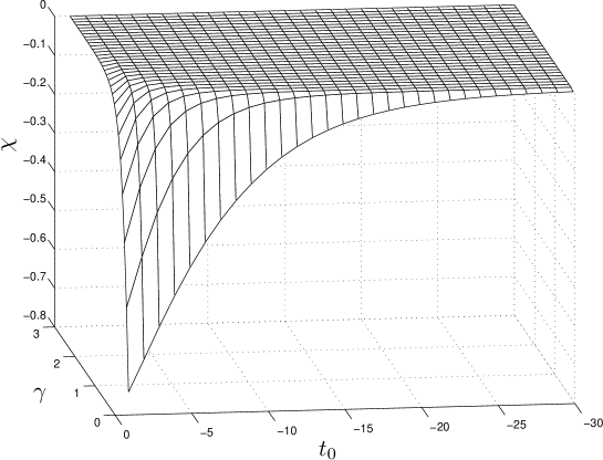
In Figure 1 the error term $\chi$ is plotted. It illustrates that for increasing spectral gap $\gamma$ and increasing time intervals $[t_{0},t_{\mathrm{f}}]$ the approximation of the SIM improves while the error decreases exponentially.

Fig. 1: The error term $\chi$ in (8) plotted against $t_{0}$ and $\gamma$ with $t_{\mathrm{f}}=0$.

3.2 Davis–Skodje Test Problem

The Davis–Skodje model (9) [6, 29] is widely used for analysis and performance tests of model reduction techniques supposed to identify slow invariant manifolds,

$$\frac{\mathrm{d}x_{1}}{\mathrm{d}t} =-x_{1}$$ (9a)

$$\frac{\mathrm{d}x_{2}}{\mathrm{d}t} =-\gamma x_{2}+\frac{(\gamma-1)x_{1}+\gamma x_{1}^{2}}{(1+x_{1})^{2}},$$ (9b)

where $\gamma>1$ is a measure for the spectral gap (stiffness) of the system. Typically model reduction algorithms show a good performance for large values of $\gamma$, which represent a large time scale separation. Small values of $\gamma$ impose a significantly harder challenge on the computation of the slow invariant manifold. For reasons of adjustable time scale separation and analytically computable SIM, the Davis–Skodje model is widely used for testing numerical model reduction approaches. We provide analytical and numerical results for the variational approach with the Davis–Skodje model.

Theorem 2.

Let $\dot{x}=f(x)$ be the Davis–Skodje model (9), the slow invariant manifold defined by $\Lambda_{\mathrm{s}}\mathrel{\mathop{:}}=\{(x_{1},x_{2})\in\mathbb{R}^{2}\ |\ x_{2}=\tfrac{x_{1}}{1+x_{1}}$} and $x^{*}$ the optimal solution of (1) with $t_{*}=t_{\mathrm{f}}\in\mathbb{R}$, $g\equiv 0$, $I_{\mathrm{fix}}=\{1\}$, and $\Phi\left(x(t)\right)=\left\|J_{f}\left(x(t)\right)\;f\left(x(t)\right)\right\|^{2}_{2}$. Then for all $\gamma>1$, $x_{1}^{t_{\mathrm{f}}}>1$ and $t_{0}<t_{\mathrm{f}}$ holds

$$\lim_{t_{0}\rightarrow-\infty}d(x^{*}(t_{\mathrm{f}}),\Lambda_{\mathrm{s}})=\lim_{t_{0}\rightarrow-\infty}\inf_{b\in\Lambda_{\mathrm{s}}}\|x^{*}(t_{\mathrm{f}})-b\|_{2}=0.$$

Proof.

The Jacobian of $f$ is given by

$$J_{f}(x(t))=\begin{pmatrix}-1&0\\ \frac{(1+\gamma)x_{1}(t)+\gamma-1}{\left(1+x_{1}(t)\right)^{3}}&-\gamma\end{pmatrix}.$$

$\Phi\left(x(t)\right)$ in the objective function can be computed explicitly as

$$\Phi\left(x(t)\right)= \left(x_{1}(t)\right)^{2}+\gamma^{4}\left(x_{2}(t)\right)^{2}+\frac{\left(x_{1}(t)\right)^{2}\left(1-2\gamma^{2}+\gamma^{4}\right)}{\left(1+x_{1}(t)\right)^{6}}$$

$$+\frac{\left(x_{1}(t)\right)^{3}\left(-2-2\gamma^{2}+4\gamma^{4}\right)}{\left(1+x_{1}(t)\right)^{6}}+\frac{\left(x_{1}(t)\right)^{4}\left(1+2\gamma^{2}+6\gamma^{4}\right)}{\left(1+x_{1}(t)\right)^{6}}$$

$$+\frac{\left(x_{1}(t)\right)^{5}\left(2\gamma^{2}+4\gamma^{4}\right)}{\left(1+x_{1}(t)\right)^{6}}+\frac{\left(x_{1}(t)\right)^{6}\gamma^{4}}{\left(1+x_{1}(t)\right)^{6}}$$

$$-x_{1}(t)x_{2}(t)\frac{\left(2\gamma^{2}x_{1}(t)-2\gamma^{2}+2\gamma^{4}+4\gamma^{4}x_{1}(t)+2\gamma^{4}\left(x_{1}(t)\right)^{2}\right)}{\left(1+x_{1}(t)\right)^{3}}.$$

An analytical solution of model (9) will be computed in the following. The first differential equation yields $x_{1}(t)=c_{1}\mathrm{e}^{-t}$ as a general solution. Equation (9b) is a inhomogeneous first order linear ordinary differential equation and the ansatz of the method of variation of parameters gives $x_{2}(t)=x_{2,\textrm{hom}}(t)+x_{2,\textrm{part}}(t)$. The homogeneous equations are solved by $x_{2,\textrm{hom}}(t)=c_{2}\mathrm{e}^{-\gamma t}$, because $\dot{x}_{2,\textrm{hom}}(t)=-\gamma c_{2}\mathrm{e}^{-\gamma t}=-\gamma x_{2,\textrm{hom}}(t)$. To determine $x_{2,\textrm{part}}(t)$ the relation

$$\mathrm{e}^{-\gamma t}\dot{c}_{2}(t)=\frac{\left(\gamma-1\right)c_{1}\mathrm{e}^{-t}+\gamma c_{1}^{2}\mathrm{e}^{-2t}}{\left(1+c_{1}\mathrm{e}^{-t}\right)^{2}}\\$$

has to be solved for $c_{2}$:

$$c_{2}(t)=\int\!\dot{c}_{2}(t)\,\textrm{d}t=\int\!\frac{\left(\gamma-1\right)c_{1}\mathrm{e}^{-t}+\gamma c_{1}^{2}\mathrm{e}^{-2t}}{\mathrm{e}^{-\gamma t}\left(1+c_{1}\mathrm{e}^{-t}\right)^{2}}\,\textrm{d}t=\frac{c_{1}\mathrm{e}^{\gamma t}}{c_{1}+\mathrm{e}^{t}}.$$

Therefore, the missing part is

$$x_{2,\textrm{part}}(t)=\mathrm{e}^{-\gamma t}\frac{c_{1}\mathrm{e}^{\gamma t}}{c_{1}+\mathrm{e}^{t}}=\frac{c_{1}}{c_{1}+\mathrm{e}^{t}}$$

and the full solution of the ODE is given by

$$x_{1}(t) =c_{1}\mathrm{e}^{-t}$$ (10a)

$$x_{2}(t) =c_{2}\mathrm{e}^{-\gamma t}+\frac{c_{1}}{c_{1}+\mathrm{e}^{t}}.$$ (10b)

Now the criterion $\Phi$ is integrated over time using (10). In the next formula $r_{i}$, $i=1,2$ represents a “rest” – all terms independent of $x_{2}(t)$, hence also independent of $c_{2}$, which annihilate after differentiation with respect to $c_{2}$ afterwards. Making use of $c_{1}=x_{1}(t_{\mathrm{f}})\;\mathrm{e}^{t_{\mathrm{f}}}=x_{1}^{t_{\mathrm{f}}}\mathrm{e}^{t_{\mathrm{f}}}$ due to (10a) yields as an expression for the objective function only depending on $c_{2}$

$$h(c_{2})= \ r_{1}+\int_{t_{0}}^{t_{\mathrm{f}}}\!\gamma^{4}\left(x_{2}(t)\right)^{2}\,\textrm{d}t$$

$$-\int_{t_{0}}^{t_{\mathrm{f}}}\!x_{1}(t)x_{2}(t)\frac{2\gamma^{2}x_{1}(t)-2\gamma^{2}+2\gamma^{4}+4\gamma^{4}x_{1}(t)+2\gamma^{4}\left(x_{1}(t)\right)^{2}}{\left(1+x_{1}(t)\right)^{3}}\,\textrm{d}t$$

$$= \ r_{2}+c_{2}^{2}\left(\frac{1}{2}\gamma^{3}\mathrm{e}^{-2\gamma t_{0}}-\frac{1}{2}\gamma^{3}\mathrm{e}^{-2\gamma t_{\mathrm{f}}}\right)$$

$$+c_{2}\int_{t_{0}}^{t_{\mathrm{f}}}\!\!\underbrace{\left[\frac{2\gamma^{4}c_{1}\mathrm{e}^{-\gamma t}}{c_{1}+\mathrm{e}^{t}}-2\gamma^{2}c_{1}\mathrm{e}^{(-1-\gamma)t}\frac{c_{1}\mathrm{e}^{-t}-1+\gamma^{2}\left(1+2c_{1}\mathrm{e}^{-t}+c_{1}^{2}\mathrm{e}^{-2t}\right)}{(1+c_{1}\mathrm{e}^{-t})^{3}}\right]}_{=\mathrel{\mathop{:}}\varphi(t)}\textrm{d}t$$

The necessary first-order condition for a minimum is applied. Setting $\tfrac{\mathrm{d}h\left(c_{2}\right)}{\mathrm{d}c_{2}}=0$ results in an optimal

$$\check{c}_{2}\mathrel{\mathop{:}}=\frac{-\int_{t_{0}}^{t_{\mathrm{f}}}\!\varphi(t)\,\mathrm{d}t}{\gamma^{3}\mathrm{e}^{-2\gamma t_{0}}-\gamma^{3}\mathrm{e}^{-2\gamma t_{\mathrm{f}}}}.$$

The second order check

$$\frac{\textrm{d}^{2}h}{\textrm{d}c_{2}^{2}}\equiv\gamma^{3}\mathrm{e}^{-2\gamma t_{0}}-\gamma^{3}\mathrm{e}^{-2\gamma t_{\mathrm{f}}}>0\quad\forall c_{2},\ t_{0}<t_{\mathrm{f}},\ \gamma>1$$

assures $\check{c}_{2}$ being a minimum.

An expression for $x_{2}(t_{\mathrm{f}})$ can be derived by substituting $c_{1}$ and $\check{c}_{2}$ in (10b):

$$x_{2}\left(t_{\mathrm{f}}\right)=\frac{-\int_{t_{0}}^{t_{\mathrm{f}}}\!\varphi(t)\,\textrm{d}t}{\gamma^{3}\mathrm{e}^{-2\gamma t_{0}}-\gamma^{3}\mathrm{e}^{-2\gamma t_{\mathrm{f}}}}\mathrm{e}^{-\gamma t_{\mathrm{f}}}+\frac{x_{1}^{t_{\mathrm{f}}}}{x_{1}^{t_{\mathrm{f}}}+1}.$$

The proof for the relation

$$\lim_{t_{0}\to-\infty}\frac{-\int_{t_{0}}^{t_{\mathrm{f}}}\!\varphi(t)\,\textrm{d}t}{\gamma^{3}\mathrm{e}^{-2\gamma t_{0}}-\gamma^{3}\mathrm{e}^{-2\gamma t_{\mathrm{f}}}}\mathrm{e}^{-\gamma t_{\mathrm{f}}}=0$$ (11)

will be given in the following Lemma 3. Because of (11) it holds

$$\lim\limits_{t_{0}\to-\infty}x_{2}(t_{\mathrm{f}})=\frac{x_{1}^{t_{\mathrm{f}}}}{x_{1}^{t_{\mathrm{f}}}+1},$$

which is the analytic expression for the slow invariant manifold of the Davis–Skodje system (see [6]). This completes the proof. ∎

Lemma 3.

Under the conditions of Theorem 2 equation (11) holds.

Proof.

In the following $\left(x\right)_{n}$ is the Pochhammer symbol which is defined as $(x)_{n}\mathrel{\mathop{:}}=x\left(x+1\right)\cdots\left(x+n-1\right)$. For the proof the integral in (11) is evaluated using Wolfram Mathematica^® 7:

$$\int_{t_{0}}^{t_{\mathrm{f}}}\!\varphi(t)\,\textrm{d}t=\left[\underbrace{\frac{-2\gamma^{2}\mathrm{e}^{\left(1-\gamma\right)t}\left(c_{1}\gamma+c_{1}+\gamma\mathrm{e}^{t}\right)}{\left(c_{1}+\mathrm{e}^{t}\right)^{2}}}_{=\mathrel{\mathop{:}}\psi_{1}(t)}\right]_{t_{0}}^{t_{\mathrm{f}}}-\left[\underbrace{\frac{\sum\limits_{n=0}^{\infty}\frac{\left(1\right)_{n}\left(1-\gamma\right)_{n}}{\left(2-\gamma\right)_{n}n!}2\gamma^{4}\mathrm{e}^{\left(1-\gamma\right)t}\frac{\mathrm{e}^{nt}}{c_{1}^{n}}}{c_{1}\left(\gamma-1\right)}}_{=\mathrel{\mathop{:}}\psi_{2}(t)}\right]_{t_{0}}^{t_{\mathrm{f}}}.$$

With this result the values of $\psi_{i}(t)$, $i=1,2$ at $t=t_{0},t_{\mathrm{f}}$ are substituted replacing the integral in equation (11) and four summands can be regarded separately in the limit:

$$\Psi_{1,t_{\mathrm{f}}}(t_{0}) \mathrel{\mathop{:}}=\frac{2\gamma^{2}\mathrm{e}^{\left(1-\gamma\right)t_{\mathrm{f}}}\left(x_{1}^{t_{\mathrm{f}}}\mathrm{e}^{t_{\mathrm{f}}}\gamma+x_{1}^{t_{\mathrm{f}}}\mathrm{e}^{t_{\mathrm{f}}}+\gamma\mathrm{e}^{t_{\mathrm{f}}}\right)\mathrm{e}^{-\gamma t_{\mathrm{f}}}}{\left(x_{1}^{t_{\mathrm{f}}}\mathrm{e}^{t_{\mathrm{f}}}+\mathrm{e}^{t_{\mathrm{f}}}\right)^{2}\left(\gamma^{3}\mathrm{e}^{-2\gamma t_{0}}-\gamma^{3}\mathrm{e}^{-2\gamma t_{\mathrm{f}}}\right)}$$

$$\Psi_{1,t_{0}}(t_{0}) \mathrel{\mathop{:}}=\frac{2\gamma^{2}\mathrm{e}^{\left(1-\gamma\right)t_{0}}\left(x_{1}^{t_{\mathrm{f}}}\mathrm{e}^{t_{\mathrm{f}}}\gamma+x_{1}^{t_{\mathrm{f}}}\mathrm{e}^{t_{\mathrm{f}}}+\gamma\mathrm{e}^{t_{0}}\right)\mathrm{e}^{-\gamma t_{\mathrm{f}}}}{\left(x_{1}^{t_{\mathrm{f}}}\mathrm{e}^{t_{\mathrm{f}}}+\mathrm{e}^{t_{0}}\right)^{2}\left(\gamma^{3}\mathrm{e}^{-2\gamma t_{0}}-\gamma^{3}\mathrm{e}^{-2\gamma t_{\mathrm{f}}}\right)}$$

$$\Psi_{2,t_{\mathrm{f}}}(t_{0}) \mathrel{\mathop{:}}=\frac{\sum\limits_{n=0}^{\infty}\frac{\left(1\right)_{n}\left(1-\gamma\right)_{n}}{\left(2-\gamma\right)_{n}n!}2\gamma^{4}\frac{\mathrm{e}^{\left(1-\gamma\right)t_{\mathrm{f}}}}{\left(x_{1}^{t_{\mathrm{f}}}\right)^{n}}\mathrm{e}^{-\gamma t_{\mathrm{f}}}}{\left(x_{1}^{t_{\mathrm{f}}}\mathrm{e}^{t_{\mathrm{f}}}\left(\gamma-1\right)\right)\left(\gamma^{3}\mathrm{e}^{-2\gamma t_{0}}-\gamma^{3}\mathrm{e}^{-2\gamma t_{\mathrm{f}}}\right)}$$

$$\Psi_{2,t_{0}}(t_{0}) \mathrel{\mathop{:}}=\frac{\sum\limits_{n=0}^{\infty}\frac{\left(1\right)_{n}\left(1-\gamma\right)_{n}}{\left(2-\gamma\right)_{n}n!}2\gamma^{4}\mathrm{e}^{\left(1-\gamma\right)t_{0}}\frac{\mathrm{e}^{nt_{0}}}{\left(x_{1}^{t_{\mathrm{f}}}\right)^{n}\mathrm{e}^{nt_{\mathrm{f}}}}\mathrm{e}^{-\gamma t_{\mathrm{f}}}}{\left(x_{1}^{t_{\mathrm{f}}}\mathrm{e}^{t_{\mathrm{f}}}\left(\gamma-1\right)\right)\left(\gamma^{3}\mathrm{e}^{-2\gamma t_{0}}-\gamma^{3}\mathrm{e}^{-2\gamma t_{\mathrm{f}}}\right)}.$$

The limit of the first two expressions $\lim_{t_{0}\to-\infty}\Psi_{1,t_{\mathrm{f}}}(t_{0})=\lim_{t_{0}\to-\infty}\Psi_{1,t_{0}}(t_{0})=0$ is evident. The two terms $\Psi_{2,t_{\mathrm{f}}}(t_{0})$ and $\Psi_{2,t_{0}}(t_{0})$ contain a hypergeometric series. $\Psi_{2,t_{\mathrm{f}}}(t_{0})$ is absolutely convergent if $x_{1}^{t_{\mathrm{f}}}>1$, $\Psi_{2,t_{0}}(t_{0})$ is absolutely convergent if $\left|{\mathrm{e}^{t_{0}}}/{x_{1}^{t_{\mathrm{f}}}\mathrm{e}^{t_{\mathrm{f}}}}\right|<1$ (generalized ratio test). This is always fullfilled for $t_{0}$ small enough. Therefore, $\lim_{t_{0}\to-\infty}\Psi_{2,t_{\mathrm{f}}}(t_{0})=\lim_{t_{0}\to-\infty}\Psi_{2,t_{0}}(t_{0})=0$. ∎

4 Numerical Results

We present numerical results for the examples investigated theoretically in the previous section. Additionally, numerical SIM computations for a simplified realistic hydrogen combustion mechanism are shown.

4.1 Numerical Methods

After suitable discretization the optimization problem (1) can be solved as a standard nonlinear programming problem (NLP), for example via the sequential quadratic programming (SQP) method [25] or interior point (IP) methods, e.g. [8]. In particular, one has to decide how to treat the differential equation constraint and the objective functional. The easiest way is a decoupled iterative approach, a full numerical integration of the ODE model with the current values of the variables subject to optimization. This procedure is called the sequential (or single shooting) approach since it fully decouples simulation of the model and optimization. However, it is often beneficial to have an “all at once” approach that couples simulation and optimization via explicit discretization of the ODE constraint. This so-called simultaneous approach has the advantage of introducing more freedom into the optimization problem since the differential equation model does not have to be solved exactly in each iteration of the optimization algorithm. Especially for highly unstable ODE problems such as (1b) considered backwards in time a fully discrete collocation approach seems appropriate for the ODE constraint. On a predefined time grid the collocation method constructs polynomials obeying the differential equation at a certain number of nodes depending on its degree. For the numerical solutions presented in this work we use a Radau-method with linear, quadratic, and cubic polynomials, respectively, [2].

The main difference between SQP and IP optimization methods for the solution of an NLP is the treatment of inequality constraints. Whereas SQP identifies the set of active constraints in the solution, IP formally couples the constraint violation to the objective function via a penalty term. Both methods finally use variants of Newton’s method applied to the necessary optimality conditions, cf. [24]. For the numerical results presented in this work the NLP has been solved using the robust interior point method implemented in IPOPT [31] including linear algebra solvers of the HSL routines [13]. The required derivatives are computed using the open source automatic differentiation package CppAD [3]. Plots are generated using MATLAB^®.

4.2 Linear Model

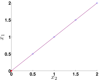
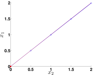
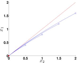
Figure 2 and Figure 3 depict numerical solution results of problem (1) with the linear model (3) and small time scale separation $\gamma=0.2$ and $\gamma=1.0$, respectively. Solutions for the forward mode and reverse mode are shown. In all cases $x_{2}$ is chosen as reaction progress variable (parameterization of the SIM) and fixed at four different values: $x_{2}^{t_{\mathrm{f}}}=2.0,$ $1.5,$ $1.0,$ $0.5$, for each of which the optimization problem is solved to obtain the coordinate of the second variable supposed to be located on the SIM (here slow eigenspace). The red curve is the SIM (slow eigenspace) which is given as the first bisectrix and the blue curves are the trajectories integrated numerically starting from those points (blue circles) that have been computed as solutions of the optimization problem. The red dot represents the equilibrium point (stable fixed point). Obviously the reverse mode gives solutions that are significantly closer to the SIM than the forward mode.

(a) Forward mode: $t_{0}=0.0,t_{\mathrm{f}}=10.0$.

(b) Reverse mode: $t_{0}=-21.0,t_{\mathrm{f}}=0.0$.

Fig. 2: Results for the linear model (4) with $\gamma=0.2$, (a) forward mode: $x_{2}(t_{0})=x_{2}^{t_{0}}$, and (b) backward mode: $x_{2}(t_{\mathrm{f}})=x_{2}^{t_{\mathrm{f}}}$.

(a) Forward mode with $t_{0}=0.0$ and $t_{\mathrm{f}}=10.0$.

(b) Reverse mode with $t_{0}=-17.0$ and $t_{\mathrm{f}}=0.0$.

Fig. 3: Results for the linear model (4) with $\gamma=1.0$, (a) forward mode: $x_{2}(t_{0})=x_{2}^{t_{0}}$, and (b) backward mode: $x_{2}(t_{\mathrm{f}})=x_{2}^{t_{\mathrm{f}}}$.

4.3 Davis–Skodje Test Problem

(a) Forward mode, $t_{0}=0.0,t_{\mathrm{f}}=10.0$.

(b) Reverse mode, $t_{0}=-8.0,t_{\mathrm{f}}=0.0$.

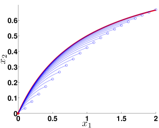
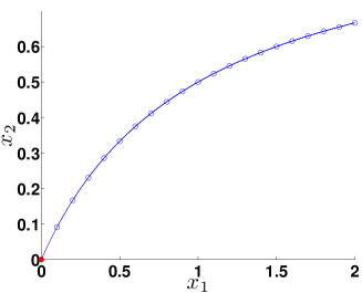
Fig. 4: Results for the Davis–Skodje test problem with (a) forward mode: $x_{1}\left(t_{0}\right)=x_{1}^{t_{0}}$, and (b) reverse mode: $x_{1}\left(t_{\mathrm{f}}\right)=x_{1}^{t_{\mathrm{f}}}$. The red curve represents the analytically calculated SIM, the blue curves are the trajectories integrated numerically from those points that are the solutions of the optimization problem (blue circles), the red dot represent the chemical equilibrium point.

Similar results are shown in Figure 4. Here the Davis–Skodje test problem is used for computations with forward mode (Fig. 4(a)) and reverse mode (Fig. 4(b)). In this case $x_{1}$ is chosen as reaction progress variable (SIM parameterization) and fixed at several values between $0.2$ and $2.0$ for the computation of SIM points as solutions of the optimization problem. The spectral gap parameter is chosen as $\gamma=1.2$.

Forward mode solutions show a larger deviation from the SIM (slow eigenspace) and a lack of invariance, whereas reverse mode solutions are highly accurate representations of the SIM.

4.4 Simplified Realistic Mechanism

As a third example numerical results for a simplified realistic mechanism for hydrogen combustion are presented. The corresponding full mechanism was originally published as a detailed hydrogen combustion mechanism by Li et al. in [20]. Ren et al. simplified the mechanism and used it for testing their ICE-PIC model reduction method in [28]. We use an adapted version of the simplified one. It consists of six chemical species (including the inert gas $\mathrm{N}_{2}$) and twelve chemical reactions as given in Table 1. Element mass conservation relations (in the general problem formulation equality constraints (1c)) for this mechanism are

$$x_{\mathrm{H}}+2x_{\mathrm{H}_{2}}+x_{\mathrm{OH}}+2x_{\mathrm{H}_{2}\mathrm{O}} =0.15$$

$$x_{\mathrm{OH}}+x_{\mathrm{O}}+x_{\mathrm{H}_{2}\mathrm{O}} =0.05$$

$$2x_{\mathrm{N}_{2}} =1.6.$$

Table 1: Adapted version of the simplified mechanism of [28]. Rate coefficients $k$ are computed in dependance of temperature $T$ as $k=AT^{b}\mathrm{exp}\left(-E_{a}/RT\right)$, where $R$ is the universal gas constant. In the mechanism $\mathrm{M}$ represents a third body being any species with collision efficiency $f_{\mathrm{H}}=1$, $f_{\mathrm{H}_{2}}=2.5$, $f_{\mathrm{OH}}=1$, $f_{\mathrm{O}}=1$, $f_{\mathrm{H}_{2}\mathrm{O}}=12$, and $f_{\mathrm{N}_{2}}=1$.

Reaction $A$ / $\text{cm},\text{mol},\text{s}$ $b$ $E_{\text{a}}$ / $\frac{\text{kJ}}{\text{mol}}$ $\mathrm{O}+\mathrm{H_{2}}$ $\rightarrow$ $\mathrm{H}+\mathrm{OH}$ $5.08\times 10^{04}$ $2.7$ $26.3$ $\mathrm{H}+\mathrm{OH}$ $\rightarrow$ $\mathrm{O}+\mathrm{H_{2}}$ $2.24\times 10^{04}$ $2.7$ $18.5$ $\mathrm{H_{2}}+\mathrm{OH}$ $\rightarrow$ $\mathrm{H_{2}O}+\mathrm{H}$ $2.16\times 10^{08}$ $1.5$ $14.4$ $\mathrm{H_{2}O}+\mathrm{H}$ $\rightarrow$ $\mathrm{H_{2}}+\mathrm{OH}$ $9.62\times 10^{08}$ $1.5$ $77.7$ $\mathrm{O}$ + $\mathrm{H_{2}O}$ $\rightarrow$ $\mathrm{2}\,\mathrm{OH}$ $2.97\times 10^{06}$ $2.0$ $56.1$ $\mathrm{2}\,\mathrm{OH}$ $\rightarrow$ $\mathrm{O}+\mathrm{H_{2}O}$ $2.94\times 10^{05}$ $2.0$ $-15.1$ $\mathrm{H_{2}}+\mathrm{M}$ $\rightarrow$ $\mathrm{2}\,\mathrm{H}+\mathrm{M}$ $4.58\times 10^{19}$ $-1.4$ $436.7$ $\mathrm{2}\,\mathrm{H}+\mathrm{M}$ $\rightarrow$ $\mathrm{H_{2}}+\mathrm{M}$ $1.18\times 10^{19}$ $-1.4$ $0.7$ $\mathrm{O}+\mathrm{H}+\mathrm{M}$ $\rightarrow$ $\mathrm{OH}+\mathrm{M}$ $4.71\times 10^{18}$ $-1.0$ $0.0$ $\mathrm{OH}+\mathrm{M}$ $\rightarrow$ $\mathrm{O}+\mathrm{H}+\mathrm{M}$ $8.07\times 10^{18}$ $-1.0$ $428.2$ $\mathrm{H}+\mathrm{OH}+\mathrm{M}$ $\rightarrow$ $\mathrm{H_{2}O}+\mathrm{M}$ $3.80\times 10^{22}$ $-2.0$ $0.0$ $\mathrm{H_{2}O}+\mathrm{M}$ $\rightarrow$ $\mathrm{H}+\mathrm{OH}+\mathrm{M}$ $6.57\times 10^{23}$ $-2.0$ $499.4$

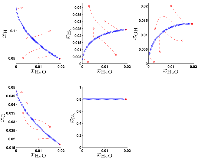
In Figure 5 results for the computation of a one-dimensional slow invariant manifold for the hydrogen combustion mechanism are shown. Solutions of the optimization problem (1) have been computed using the reverse mode. Again the red dot represents the chemical equilibrium and the progress variable $x_{\mathrm{H}_{2}\mathrm{O}}$ has been fixed at different values between $0.0005$ and $0.0180$. The blue circles are the final values $x(t_{\mathrm{f}})$ of the solution trajectories of the optimization problem and blue curves are the trajectories integrated numerically from those values forward to equilibrium. They accurately approximate the SIM; convergence of trajectories (dashed red curves) started from arbitrary initial values (red circles) to the computed SIM is visualized in Figure 5.

Fig. 5: Results for a one-dimensional SIM of the simplified combustion mechanism computed with reverse mode, i.e. $x_{\mathrm{H}_{2}\mathrm{O}}\left(t_{\mathrm{f}}\right)=x_{\mathrm{H}_{2}\mathrm{O}}^{t_{\mathrm{f}}}$. $t_{0}=-0.0004,t_{\mathrm{f}}=0.0$, temperature $T=3000~{}{\rm K}$. Arbitrary trajectories relax on the manifold (red, dashed).

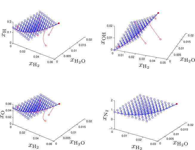
Figure 6 shows a two-dimensional manifold computed with the reverse mode. Two reaction progress variables $x_{\mathrm{H}_{2}\mathrm{O}}$ and $x_{\mathrm{H}_{2}}$ are fixed and the slow invariant manifold is approximated on a two-dimensional grid as a solution of a family of optimization problems.

Fig. 6: Results for two-dimensional SIM of the simplified combustion mechanism computed with reverse mode and $x_{\mathrm{H}_{2}\mathrm{O}}(t_{\mathrm{f}})$ and $x_{\mathrm{H}_{2}}(t_{\mathrm{f}})$ chosen as reaction progress variables, $t_{0}=-5.0\times 10^{-7},t_{\mathrm{f}}=0.0$, constant temperature $T=3000~{}{\rm K}$. The same arbitrary trajectories as in Fig. 5 are shown in red.

References

• [1] A. Adrover, F. Creta, M. Giona, and M. Valorani, Stretching-based diagnostics and reduction of chemical kinetic models with diffusion, J. Comput. Phys., 225 (2007), pp. 1442–1471.
• [2] U.M. Ascher and L.R. Petzold, Computer methods for ordinary differential equations and differential-algebraic equations, SIAM, Philadelphia, 1998.
• [3] B.M. Bell and J.V. Burke, Algorithmic differentiation of implicit functions and optimal values, in Advances in Automatic Differentiation, Ch.H. Bischof, H.M. Bücker, P.D. Hovland, U. Naumann, and J. Utke, eds., Springer, 2008, pp. 67–77.
• [4] V. Bykov, V. Gol’dshtein, and U. Maas, Simple global reduction technique based on decomposition approach, Combust. Theor. Model., 12 (2008), pp. 389–405.
• [5] E. Chiavazzo, I.V. Karlin, A.N. Gorban, and K. Boulouchos, Combustion simulation via lattice boltzmann and reduced chemical kinetics, J. Stat. Mech., 2009 (2009), p. P06013.
• [6] M.J. Davis and R.T. Skodje, Geometric investigation of low-dimensional manifolds in systems approaching equilibrium, J. Chem. Phys., 111 (1999), pp. 859–874.
• [7] S. Delhaye, L.M.T. Somers, J.A. van Oijen, and L.P.H. de Goey, Simulating transient effects of laminar diffusion flames using flamelet libraries, in Proceedings of the Third European Combustion Meeting, ECM, 2007.
• [8] A. Forsgren, P.E. Gill, and M.H. Wright, Interior methods for nonlinear optimization, SIAM Rev., 44 (2002), pp. 525–597.
• [9] S.J. Fraser, The steady state and equilibrium approximations: A geometrical picture, J. Chem. Phys., 88 (1988), pp. 4732–4738.
• [10] C.W. Gear, T.J. Kaper, I.G. Kevrekidis, and A. Zagaris, Projecting to a slow manifold: Singularly perturbed systems and legacy codes, SIAM J. Appl. Dyn. Syst., 4 (2005), pp. 711–732.
• [11] A.N. Gorban and I.V. Karlin, Invariant Manifolds for Physical and Chemical Kinetics, vol. 660 of Lecture Notes in Physics, Springer-Verlag Berlin, 2005.
• [12] A. Gorban, I. Karlin, and A. Zinovyev, Invariant grids: Method of complexity reduction in reaction networks, Complexus, 2 (2005), pp. 110–127.
• [13] HSL, A collection of fortran codes for large-scale scientific computation. See URL http://www.hsl.rl.ac.uk, 2007.
• [14] J.C. Keck and D. Gillespie, Rate-controlled partial-equilibrium method for treating reacting gas mixtures, Combust. Flame, 17 (1971), pp. 237–241.
• [15] S.H. Lam, Recent Advances in the Aerospace Sciences, Plenum Press, New York and London, 1985, ch. Singular Perturbation for Stiff Equations using Numerical Methods, pp. 3–20.
• [16] S.H. Lam and D.A. Goussis, The CSP method for simplifying kinetics, Int. J. Chem. Kinet., 26 (1994), pp. 461–486.
• [17] D. Lebiedz, Computing minimal entropy production trajectories: An approach to model reduction in chemical kinetics, J. Chem. Phys., 120 (2004), pp. 6890–6897.
• [18] D. Lebiedz, V. Reinhardt, and J. Kammerer, Novel trajectory based concepts for model and complexity reduction in (bio)chemical kinetics, in Model reduction and coarse-graining approaches for multi-scale phenomena, A. N. Gorban, N. Kazantzis, I. G. Kevrekidis, and C. Theodoropoulos, eds., Springer, Berlin, 2006, pp. 343–364.
• [19] D. Lebiedz, V. Reinhardt, and J. Siehr, Minimal curvature trajectories: Riemannian geometry concepts for model reduction in chemical kinetics. arXiv:0910.3527, 2009.
• [20] J. Li, Z. Zhao, A. Kazakov, and F.L. Dryer, An updated comprehensive kinetic model of hydrogen combustion, Int. J. Chem. Kinet., 36 (2004), pp. 566–575.
• [21] U. Maas and S.B. Pope, Simplifying chemical kinetics: Intrinsic low-dimensional manifolds in composition space, Combust. Flame, 88 (1992), pp. 239–264.
• [22] K.D. Mease, S. Bharadwaj, and S. Iravanchy, Timescale analysis for nonlinear dynamical systems, Journal of Guidance, Control, and Dynamics, 26 (2003), pp. 318–330.
• [23] A.H. Nguyen and S.J. Fraser, Geometrical picture of reaction in enzyme kinetics, J. Chem. Phys., 91 (1989), pp. 186–193.
• [24] J. Nocedal and S.J. Wright, Numerical Optimization, Springer Series in Operations Research and Financial Engineering, Springer, New York, second ed., 2006.
• [25] M.J.D. Powell, A fast algorithm for nonlinearly constrained optimization calculations, in Numerical Analysis, A. Dold and B. Eckmann, eds., vol. 630 of Lecture Notes in Mathematics, Springer-Verlag Berlin, 1978, pp. 144–157.
• [26] V. Reinhardt, M. Winckler, and D. Lebiedz, Approximation of slow attracting manifolds in chemical kinetics by trajectory-based optimization approaches, J. Phys. Chem. A., 112 (2008), pp. 1712–1718.
• [27] Z. Ren and S.B. Pope, Species reconstruction using pre-image curves, in Proc. Comb. Inst., vol. 30, 2005, pp. 1293–1300.
• [28] Z. Ren, S.B. Pope, A. Vladimirsky, and J.M. Guckenheimer, The invariant constrained equilibrium edge preimage curve method for the dimension reduction of chemical kinetics, J. Chem. Phys., 124 (2006), p. 114111.
• [29] S. Singh, J.M. Powers, and S. Paolucci, On slow manifolds of chemically reactive systems, J. Chem. Phys., 117 (2002), pp. 1482–1496.
• [30] J.A. van Oijen and L.P.H. de Goey, Modelling of premixed laminar flames using flamelet-generated manifolds, Combust. Sci. Technol., 161 (2000), pp. 113–137.
• [31] A. Wächter and L.T. Biegler, On the implementation of a primal-dual interior point filter line search algorithm for large-scale nonlinear programming, Math. Program., 106 (2006), pp. 25–57.
• [32] J. Warnatz, U. Maas, and R.W. Dibble, Combustion: Physical and Chemical Fundamentals, Modeling and Simulation, Experiments, Pollutant Formation, Springer, Berlin, 2006.
• [33] A. Zagaris, C.W. Gear, T.J. Kaper, and Y.G. Kevrekidis, Analysis of the accuracy and convergence of equation-free projection to a slow manifold, ESAIM: Math. Model. Numer. Anal., 43 (2009), pp. 757–784.