Abstract

The electroweak currents of quarks and leptons in the $SO(5)\times U(1)$ gauge-Higgs unification model in the Randall-Sundrum warped space are determined. The 4D gauge couplings deviate from those in the standard model and the weak universality is slightly violated. It is shown that the model is free from 4D anomalies and the deviations of the gauge couplings are tiny, less than 1% except for the top quark. The $Zt_{L}\bar{t}_{L}$, $Zt_{R}\bar{t}_{R}$, $Zb_{L}\bar{b}_{L}$ and $Zb_{R}\bar{b}_{R}$ couplings deviate from those in the standard model by $-7$%, 18%, 0.3% and 0.9% with the warp factor $z_{L}=10^{15}$, respectively. The violation of the $\mu$-$e$, $\tau$-$e$ and $t$-$e$ universality in the charged current interactions is ${\cal O}(10^{-8})$, ${\cal O}(10^{-6})$ and 2.3%, respectively.

1 Introduction

The Higgs boson is the only particle yet to be found in the standard model of electroweak interactions. It is not clear, however, if the Higgs boson appears as described in the standard model. New physics may be hidden behind it.

In the gauge-Higgs unification scenario the 4D Higgs field is identified with a part of the extra-dimensional component of gauge fields in higher dimensions.[2, 3] The 4D Higgs field appears as an Aharonov-Bohm (AB) phase, or a Wilson line phase, in the extra dimension.[4, 5, 6] The electroweak (EW) symmetry breaking is induced by dynamics of the AB phase through the Hosotani mechanism. A finite mass of the Higgs boson is generated at the quantum level, the mechanism of which provides a new way of solving the gauge hierarchy problem as an alternative to supersymmetric theories, the little Higgs model and the Higgsless model.[7]

A realistic gauge-Higgs unification model is constructed in the Randall-Sundrum warped space.[8, 9, 10] Based on the gauge group $SO(5)\times U(1)$ quarks and leptons are introduced in the vector (5) representation of $SO(5)$ in the bulk five-dimensional spacetime with additional fermions localized on the Planck brane.[11]-[14] The presence of the top quark dynamically induces the EW symmetry breaking, thereby the effective potential $V_{\rm eff}$ for the AB phase $\theta_{H}$ being minimized at $\theta_{H}=\pm\hbox{${1\over 2}$}\pi$.[13]

In the gauge-Higgs unification scenario the interactions of the Higgs boson are governed by the gauge principle. Its interactions with other particles deviate from those in the standard model, which may be understood as manifestation of the underlying gauge invariance. The 4D neutral Higgs field $H(x)$ corresponds to four-dimensional fluctuations of the AB phase $\theta_{H}$ so that these two appear, in the effective theory at low energies, always in the combination of

$$\hat{\theta}_{H}(x)=\theta_{H}+\frac{H(x)}{f_{H}}$$ (1.1)

where $f_{H}$ turns out $\sim 246\,$GeV. The effective interactions with $W$, $Z$ bosons and fermions are summarized as [14]

$${\cal L}_{\rm eff}=-V_{\rm eff}(\hat{\theta}_{H})-m_{W}^{2}(\hat{\theta}_{H})W^{\dagger}_{\mu}W^{\mu}-\hbox{${1\over 2}$}m_{Z}^{2}(\hat{\theta}_{H})Z_{\mu}Z^{\mu}-\sum_{a,b}m^{F}_{ab}(\hat{\theta}_{H})\psi\kern-6.49994pt\raise 6.00006pt\hbox{$-$}_{a}\psi_{b}~{}.$$ (1.2)

The mass functions are approximately given by $m_{W}(\hat{\theta}_{H})\sim\hbox{${1\over 2}$}gf_{H}\sin\hat{\theta}_{H}$, $m^{F}_{f}(\hat{\theta}_{H})\sim y_{f}f_{H}\sin\hat{\theta}_{H}$ etc. In the standard model they are given by $m_{W}=\hbox{${1\over 2}$}g(v+H)$ and $m^{F}_{f}=y_{f}(v+H)$. The periodicity in $\hat{\theta}_{H}$ in the gauge-Higgs unification follows from the gauge invariance of the theory.

The large gauge invariance implying the periodicity in $\hat{\theta}_{H}$, and the smooth $\hat{\theta}_{H}$-dependence of the mass functions without the level crossing in the warped space lead to significant deviation in the Higgs couplings from the standard model.[14]-[20] As follows from (1.2), the $WWH$, $ZZH$ and Yukawa couplings are suppressed by a factor $\sim\cos\theta_{H}$ compared with those in the standard model. At particular values of $\theta_{H}=\pm\hbox{${1\over 2}$}\pi$, namely at the extrema of the smooth periodic mass functions, they vanish. As proven in ref. [21] the $WWH^{\ell}$, $ZZH^{\ell}$ and $\psi\kern-6.49994pt\raise 6.00006pt\hbox{$-$}\psi H^{\ell}$ couplings with an odd integer $\ell$ vanish to all order in perturbation theory, provided that all bulk fermions belong to the vector representation of $SO(5)$. The Higgs boson becomes absolutely stable, the stability being protected by the dynamically emerging $H$-parity. The Higgs boson is $H$-parity odd, while all other particles in the standard model are $H$-parity even. This leads to astonishing physical consequences. In the evolution of the universe, Higgs bosons become the cold dark matter. The dark matter density observed at WMAP is explained with $m_{H}\sim 70\,$GeV. This scenario of the stable Higgs bosons as cold dark matter is quite different from the Kaluza-Klein (KK) dark matter scenario in which additional fields with odd KK parity become dark matter.[22] The LEP2 bound for $m_{H}$ is evaded as the $ZZH$ coupling vanishes. Higgs bosons can be produced in pairs in collider experiments . They appear as missing energies and momenta.

In this paper we turn our attention to the gauge couplings of quarks and leptons.[23, 24] Although the five-dimensional gauge couplings are dictated by the gauge principle and are universal, the four-dimensional gauge couplings appear as overlap integrals in the fifth coordinate with wave functions of relevant fields inserted. In the gauge-Higgs unification models in the RS warped space each of the left- and right-handed quarks and leptons has a quite different profile of the wave function so that deviation from the standard model is expected to arise in gauge couplings as well. It has been argued that in the $SU(3)$ model the weak ($\mu$-$e$, $\tau$-$e$) universality is slightly violated.[25] There appear corrections to the $S$ and $T$ parameters,[11, 26, 27] which would constrain the models. Consequences in the tree level unitarity in the $WW$, $WZ$, and $ZZ$ scattering also have been discussed.[28]-[31] Further, it has been shown that corrections to muon anomalous magnetic moment and to neutron electric dipole moment appear in the $SU(3)$ model, which has been used to get a bound for the KK mass scale.[32, 33]

The purpose of this paper is to determine the $W$, $Z$ and electromagnetic currents in the $SO(5)\times U(1)$ model with three generations of quarks and leptons, which generalizes the model of ref. [13]. The electroweak currents depend on the profiles of wave functions of $W$, $Z$, quarks and leptons both in the fifth dimension and in the $SO(5)$ group. Despite their highly nontrivial profiles, it is found that the deviations of the couplings of quarks and leptons to the gauge bosons from the standard model are less than 1% except for the top quark.

The paper is organized as follows. In Section 2 the $SO(5)\times U(1)$ model is specified. Quark and lepton multiplets are introduced in the bulk five-dimensional spacetime, with associated fermions localized on the Planck brane. In Section 3 we show that with both quark and lepton multiplets included the model becomes free from 4D anomalies with respect to the $SO(4)\times U(1)$ gauge symmetry left after the orbifold conditions imposed. Brane fermions play an important role there. In Section 4 the spectrum of gauge bosons and fermions is determined, and the wave functions of the photon, $W$, $Z$, quarks, and leptons are determined. Numerical values of the coefficients in the wave functions are give at $\theta_{H}=\hbox{${1\over 2}$}\pi$. By making use of the wave functions, the electroweak gauge couplings are evaluated in Section 5. Comparison with those in the standard model is given. Section 6 is devoted to discussions and conclusion. Useful formulas are collected in appendices A, B, and C. The results for the gauge couplings evaluated with the pole masses of quarks and leptons are given in the main text, while the results with the running quark and lepton masses at the $m_{Z}$ scale are summarized in Appendix D.

2 Model

The model is defined in the Randall-Sundrum (RS) warped spacetime whose metric is given by

$$ds^{2}=G_{MN}dx^{M}dx^{N}=e^{-2\sigma(y)}\eta_{\mu\nu}dx^{\mu}dx^{\nu}+dy^{2},\qquad$$ (2.1)

where $\eta_{\mu\nu}=\textrm{diag}(-1,1,1,1)$, $\sigma(y)=\sigma(y+2L)$, and $\sigma(y)=k|y|$ for $|y|\leq L$. The fundamental region in the fifth dimension is given by $0\leq y\leq L$. The Planck brane and the TeV brane are located at $y=0$ and $y=L$, respectively. The bulk region $0<y<L$ is an anti-de Sitter spacetime with the cosmological constant $\Lambda=-6k^{2}$.

We consider an $SO(5)\times U(1)_{X}$ gauge theory in the RS warped spacetime. The $SO(5)\times U(1)_{X}$ symmetry is broken to $SO(4)\times U(1)_{X}$ by the orbifold boundary conditions at the Planck and TeV branes. The symmetry is spontaneously broken to $SU(2)_{L}\times U(1)_{Y}$ by additional interactions at the Planck brane.

The action integral consists of four parts:

$$S=S_{\textrm{\scriptsize bulk}}^{\textrm{\scriptsize gauge}}+S_{\textrm{\scriptsize Pl. brane}}^{\textrm{\scriptsize scalar}}+S_{\textrm{\scriptsize bulk}}^{\textrm{\scriptsize fermion}}+S_{\textrm{\scriptsize Pl. brane}}^{\textrm{\scriptsize fermion}}.$$ (2.2)

The bulk parts respect $SO(5)\times U(1)_{X}$ gauge symmetry. There are $SO(5)$ gauge fields $A_{M}$ and $U(1)_{X}$ gauge field $B_{M}$. The former are decomposed as $A_{M}=\sum_{I=1}^{10}A_{M}^{I}T^{I}=\sum_{a_{L}=1}^{3}A_{M}^{a_{L}}T^{a_{L}}+\sum_{a_{R}=1}^{3}A_{M}^{a_{R}}T^{a_{R}}+\sum_{\hat{a}=1}^{4}A_{M}^{\hat{a}}T^{\hat{a}}$, where $T^{a_{L},a_{R}}(a_{L},a_{R}=1,2,3)$ and $T^{\hat{a}}(\hat{a}=1,\ldots,4)$ are the generators of $SO(4)\sim SU(2)_{L}\times SU(2)_{R}$ and $SO(5)/SO(4)$, respectively. In a vectorial representation, the components of the generator are $T_{ij}^{a_{L},a_{R}}=-{i\over 2}[{1\over 2}\epsilon^{abc}(\delta_{i}^{b}\delta_{j}^{c}-\delta_{j}^{b}\delta_{i}^{c})\pm(\delta_{i}^{a}\delta_{j}^{4}-\delta_{j}^{a}\delta_{i}^{4})]$ and $T_{ij}^{\hat{a}}=-{i\over\sqrt{2}}(\delta_{i}^{\hat{a}}\delta_{j}^{5}-\delta_{j}^{\hat{a}}\delta_{i}^{5})$, where $i,j=1,\ldots,5$. They satisfy $\textrm{Tr}(T^{I}T^{J})=\delta^{IJ}$. The action integral for the pure gauge boson part is

$$S_{\rm bulk}^{\rm gauge} \!\!\!=\!\!\! \int d^{5}x\sqrt{-G}\left[-\textrm{tr}({1\over 4}F^{(A)MN}F_{MN}^{(A)}+{1\over 2\xi}(f_{\textrm{\scriptsize gf}}^{(A)})^{2}+{\cal L}_{\textrm{\scriptsize gh}}^{(A)})\right.$$ (2.3)

$$\qquad\left.-({1\over 4}F^{(B)MN}F_{MN}^{(B)}+{1\over 2\xi}(f_{\textrm{\scriptsize gf}}^{(B)})^{2}+{\cal L}_{\textrm{\scriptsize gh}}^{(B)})\right],$$

where the gauge fixing and ghost terms are denoted as functionals with suffices gf and gh, respectively. Here $F_{MN}^{(A)}=\partial_{M}A_{N}-\partial_{N}A_{M}-ig_{A}[A_{M},A_{N}]$ and $F_{MN}^{(B)}=\partial_{M}B_{N}-\partial_{N}B_{M}$.

The orbifold boundary conditions at $y_{0}=0$ and $y_{1}=L$ for gauge fields are given by

$$\left(\begin{array}[]{c}A_{\mu}\\ A_{y}\\ \end{array}\right)(x,y_{j}-y)=P_{j}\left(\begin{array}[]{c}A_{\mu}\\ -A_{y}\\ \end{array}\right)(x,y_{j}+y)P_{j}^{-1},$$ (2.8)

$$\left(\begin{array}[]{c}B_{\mu}\\ B_{y}\\ \end{array}\right)(x,y_{j}-y)=\left(\begin{array}[]{c}B_{\mu}\\ -B_{y}\\ \end{array}\right)(x,y_{j}+y),$$ (2.13)

$$P_{j}=\textrm{diag}(-1,-1,-1,-1,+1),\qquad(j=0,1),$$ (2.14)

which reduce the $SO(5)\times U(1)_{X}$ symmetry to $SO(4)\times U(1)_{X}$. A scalar field $\Phi(x)$ on the Planck brane belongs to $(0,{1\over 2})$ representation of $SO(4)\sim SU(2)_{L}\times SU(2)_{R}$ with a $U(1)_{X}$ charge. With the brane action

$$S_{\textrm{\scriptsize Pl. brane}}^{\textrm{\scriptsize scalar}} \!\!\!=\!\!\! \int d^{5}x\delta(y)\left\{-(D_{\mu}\Phi)^{\dagger}D^{\mu}\Phi-\lambda_{\Phi}(\Phi^{\dagger}\Phi-w^{2})^{2}\right\},$$

$$D_{\mu}\Phi \!\!\!=\!\!\! \partial_{\mu}\Phi-i\left(g_{A}\sum_{a_{R}}^{3}A_{\mu}^{a_{R}}T^{a_{R}}+{g_{B}\over 2}B_{\mu}\right)\Phi,$$ (2.15)

the $SU(2)_{R}\times U(1)_{X}$ symmetry breaks down to $U(1)_{Y}$, the weak hypercharge in the standard model. Let us denote

$$\hskip-28.45274pt\left(\begin{array}[]{c}A_{M}^{{}^{\prime}3_{R}}\\ A_{M}^{Y}\\ \end{array}\right)=\left(\begin{array}[]{cc}c_{\phi}&-s_{\phi}\\ s_{\phi}&c_{\phi}\\ \end{array}\right)\left(\begin{array}[]{c}A_{M}^{3_{R}}\\ B_{M}\\ \end{array}\right)$$ (2.22)

$$\hskip-28.45274ptc_{\phi}={g_{A}\over\sqrt{g_{A}^{2}+g_{B}^{2}}},\quad s_{\phi}={g_{B}\over\sqrt{g_{A}^{2}+g_{B}^{2}}}~{}.$$ (2.23)

Suppose that $w$ is much larger than the KK mass scale $M_{\rm KK}$, being of, for instance, ${\cal O}(M_{\textrm{\scriptsize GUT}})$ to ${\cal O}(M_{\textrm{\scriptsize Planck}})$. Although the fields $A_{\mu}^{1_{R}}$, $A_{\mu}^{2_{R}}$ and $A_{\mu}^{{}^{\prime}3_{R}}$ are even under parity and obey the Neumann condition, the values at $y=0$ of low-lying modes of their KK towers become extremely tiny because of the large VEV $w$. The net effect for the low-lying modes of the KK towers of $A_{\mu}^{1_{R}}$, $A_{\mu}^{2_{R}}$ and $A_{\mu}^{{}^{\prime}3_{R}}$ is that they effectively obey Dirichlet boundary conditions at the Planck brane so that the originally-massless modes of $A_{\mu}^{1_{R}}$, $A_{\mu}^{2_{R}}$ and $A_{\mu}^{{}^{\prime}3_{R}}$ acquire large masses of ${\cal O}(M_{\rm KK})$.[18] On the other hand the fields $A_{y}^{1_{R}}$, $A_{y}^{2_{R}}$ and $A_{y}^{{}^{\prime}3_{R}}$ are odd under parity and necessarily vanish at $y=0$. The effective orbifold boundary conditions are tabulated in Table 1. In passing, it is possible to allow discontinuities in $A_{y}$ at $y=0$ by enlarging the configuration space for $A_{y}$ as discussed in ref. [34]. One can include discontinuities in $A_{y}$ in the gauge-fixing condition at the Planck brane. Then $A_{y}$ can obey either Dirichlet, or Neumann, or other boundary condition, depending on the gauge condition, as spelled out in refs. [13] and [34]. We adopt the viewpoint that all vector potentials $A_{M}$ are continuous, but the results in the present paper are not affected by the gauge choice.

Table 1: Boundary conditions of gauge fields and bulk fermions: The effective Dirichlet condition resulting from brane dynamics is denoted as D_eff. For fermions $\psi_{aj}$, $j=1,\cdots,4$.

$A_{\mu}^{a_{L}}$	$A_{\mu}^{1_{R},2_{R}}$	$A_{\mu}^{{}^{\prime}3_{R}}$	$A_{\mu}^{Y}$	$A_{\mu}^{\hat{a}}$	$B_{\mu}$	$\psi_{ajL},\psi_{a5R}$
(N,N)	(Deff,N)	(Deff,N)	(N,N)	(D,D)	(N,N)	(N,N)
$A_{y}^{a_{L}}$	$A_{y}^{1_{R},2_{R}}$	$A_{y}^{{}^{\prime}3_{R}}$	$A_{y}^{Y}$	$A_{y}^{\hat{a}}$	$B_{y}$	$\psi_{ajR},\psi_{a5L}$
(D,D)	(D,D)	(D,D)	(D,D)	(N,N)	(D,D)	(D,D)

Bulk fermions for quarks and leptons are introduced as multiplets in the vectorial representation of $SO(5)$. In the quark sector two vector multiplets are introduced for each generation. In the lepton sector it suffices to introduce one multiplet for each generation to describe massless neutrinos, whereas it is necessary to introduce two multiplets to describe massive neutrinos. They are denoted by $\Psi_{a}^{t}=(\psi_{a1},\ldots,\psi_{a5})^{t}$ where the subscript $a$ runs from 1 to 3 or 4 for each generation.

The action integral in the bulk is given by

$$S_{\textrm{\scriptsize bulk}}^{\textrm{\scriptsize fermion}} \!\!\!=\!\!\! \int d^{5}x\,\sqrt{-G}\sum_{a}i\bar{\Psi}_{a}{\cal D}(c_{a})\Psi_{a}~{},$$ (2.24)

$${\cal D}(c_{a}) \!\!\!=\!\!\! \Gamma^{A}e_{A}^{M}(\partial_{M}+{1\over 8}\omega_{MBC}[\Gamma^{B},\Gamma^{C}]-ig_{A}A_{M}-ig_{B}Q_{Xa}B_{M})-c_{a}\sigma^{\prime}(y)~{},$$ (2.25)

where the Dirac conjugate is given by $\bar{\Psi}=i\Psi^{\dagger}\Gamma^{0}$ and $\Gamma^{\mu}$ matrices are given by

$$\Gamma^{\mu}=\left(\begin{array}[]{cc}&\sigma^{\mu}\\ \bar{\sigma}^{\mu}&\\ \end{array}\right),\quad\Gamma^{5}=\left(\begin{array}[]{cc}1&\\ &-1\\ \end{array}\right),\quad\sigma^{\mu}=(1,\vec{\sigma}),\quad\bar{\sigma}^{\mu}=(-1,\vec{\sigma}).$$ (2.30)

The non-vanishing spin connection is $\omega_{\mu m5}=-\sigma^{\prime}e^{-\sigma}\delta_{\mu m}$, where $\delta_{\mu m}$ denotes a vierbein in the 4D Minkowski spacetime. The $c_{a}$ term in Eq. (2.25) gives a bulk kink mass, where $\sigma^{\prime}(y)=k\epsilon(y)$ is a periodic step function with a magnitude $k$. The dimensionless parameter $c_{a}$ plays an important role in the RS warped spacetime. The orbifold boundary conditions are given by

$$\Psi_{a}(x,y_{j}-y) \!\!\!=\!\!\! P_{j}\Gamma^{5}\Psi_{a}(x,y_{j}+y).$$ (2.31)

With $P_{j}$ in Eq. (2.14), the first four component of $\Psi_{a}$ are even under parity for the 4D left-handed $(\Gamma^{5}=-1)$ components, whereas the fifth component of $\Psi_{a}$ is even for the 4D right-handed component. An $SO(5)$ vector $\Psi$ can be expressed as the sum of $({1\over 2},{1\over 2})$ representation and a singlet $(0,0)$ of the subgroup $SU(2)_{L}\times SU(2)_{R}$. The $({1\over 2},{1\over 2})$ representation is expressed as

$$\hat{\psi} \!\!\!=\!\!\! \begin{pmatrix}\hat{\psi}_{11}&\hat{\psi}_{12}\cr\hat{\psi}_{21}&\hat{\psi}_{22}\end{pmatrix}=\frac{1}{\sqrt{2}}(\psi_{4}+i\vec{\psi}\cdot\vec{\sigma})i\sigma_{2}$$ (2.32)

$$\!\!\!=\!\!\! -\frac{1}{\sqrt{2}}\begin{pmatrix}\psi_{2}+i\psi_{1}&-(\psi_{4}+i\psi_{3})\\ \psi_{4}-i\psi_{3}&\psi_{2}-i\psi_{1}\\ \end{pmatrix}~{}.$$ (2.33)

$\psi_{5}$ is a singlet $(0,0)$. The quarks in the third generation, for instance, are composed of bulk Dirac fermions in the $SO(5)$ vectorial representation

$$\Psi_{1} \!\!\!=\!\!\! \left[Q_{1}=\left(\begin{array}[]{c}T\\ B\\ \end{array}\right),~{}q=\left(\begin{array}[]{c}t\\ b\\ \end{array}\right),~{}t^{\prime}\right],$$ (2.38)

$$\Psi_{2} \!\!\!=\!\!\! \left[Q_{2}=\left(\begin{array}[]{c}U\\ D\\ \end{array}\right),~{}Q_{3}=\left(\begin{array}[]{c}X\\ Y\\ \end{array}\right),~{}b^{\prime}\right],$$ (2.43)

and right-handed brane fermions of the $({1\over 2},0)$ representation in $SU(2)_{L}\times SU(2)_{R}$

$$\hat{\chi}_{1R}=\left(\begin{array}[]{c}\hat{T}_{R}\\ \hat{B}_{R}\\ \end{array}\right),\qquad\hat{\chi}_{2R}=\left(\begin{array}[]{c}\hat{U}_{R}\\ \hat{D}_{R}\\ \end{array}\right),\qquad\hat{\chi}_{3R}=\left(\begin{array}[]{c}\hat{X}_{R}\\ \hat{Y}_{R}\\ \end{array}\right).$$ (2.50)

For brane fermions, the hypercharge $Y/2$ is equal to the $U(1)_{X}$ charge, $Q_{X}$. Leptons in the third generation (with massless $\nu_{\tau}$) are composed of bulk Dirac fermions in the $SO(5)$ vectorial representation

$$\Psi_{3}=\left[\ell=\left(\begin{array}[]{c}\nu_{\tau}\\ \tau\\ \end{array}\right),~{}L_{1}=\left(\begin{array}[]{c}L_{1X}\\ L_{1Y}\\ \end{array}\right),~{}\tau^{\prime}\right],$$ (2.55)

and right-handed brane fermions of the $({1\over 2},0)$ representation in $SU(2)_{L}\times SU(2)_{R}$

$$\hat{\chi}_{1R}^{\ell}=\left(\begin{array}[]{c}\hat{L}_{1XR}\\ \hat{L}_{1YR}\\ \end{array}\right).$$ (2.58)

The assignment of charges for quarks and leptons is tabulated in Table 2, where the $U(1)_{X}$ charge, the hypercharge and the electric charge are denoted as $Q_{X}$, $Y/2=T^{3_{R}}+Q_{X}$ and $Q_{E}=T^{3_{L}}+T^{3_{R}}+Q_{X}$, respectively.

Table 2: Content of bulk and brane fermions in the third generation. The brane fermion $\hat{\chi}_{2R}$ couples to both $q$ and $Q_{2}$ so that it may be placed in the column of $\Psi_{1}$ instead of $\Psi_{2}$.

bulk	$Q_{X}$		$\hbox{${1\over 2}$}Y$	$Q_{E}$	on the brane	$Q_{X},\hbox{${1\over 2}$}Y$	$Q_{E}$
$\Psi_{1}$	${2/3}$	$Q_{1}=\left(\begin{array}[]{c}T\\ B\\ \end{array}\right)$	${7/6}$	$\begin{array}[]{c}{5/3}\\ {2/3}\\ \end{array}$	$\hat{\chi}_{1R}=\left(\begin{array}[]{c}\hat{T}_{R}\\ \hat{B}_{R}\\ \end{array}\right)$	${7/6}$	$\begin{array}[]{c}{5/3}\\ {2/3}\\ \end{array}$
		$q=\left(\begin{array}[]{c}t\\ b\\ \end{array}\right)$	${1/6}$	$\begin{array}[]{c}{2/3}\\ -{1/3}\\ \end{array}$
		$t^{\prime}$	${2/3}$	${2/3}$
$\Psi_{2}$	$-{1/3}$	$Q_{2}=\left(\begin{array}[]{c}U\\ D\\ \end{array}\right)$	${1/6}$	$\begin{array}[]{c}{2/3}\\ -{1/3}\\ \end{array}$	$\hat{\chi}_{2R}=\left(\begin{array}[]{c}\hat{U}_{R}\\ \hat{D}_{R}\\ \end{array}\right)$	${1/6}$	$\begin{array}[]{c}{2/3}\\ -{1/3}\\ \end{array}$
		$Q_{3}=\left(\begin{array}[]{c}X\\ Y\\ \end{array}\right)$	$-{5/6}$	$\begin{array}[]{c}-{1/3}\\ -{4/3}\\ \end{array}$	$\hat{\chi}_{3R}=\left(\begin{array}[]{c}\hat{X}_{R}\\ \hat{Y}_{R}\\ \end{array}\right)$	$-{5/6}$	$\begin{array}[]{c}-{1/3}\\ -{4/3}\\ \end{array}$
		$b^{\prime}$	$-{1/3}$	$-{1/3}$
$\Psi_{3}$	$-1$	$\ell=\left(\begin{array}[]{c}\nu_{\tau}\\ \tau\\ \end{array}\right)$	$-{1/2}$	$\begin{array}[]{c}0\\ -1\\ \end{array}$
		$L_{1}=\left(\begin{array}[]{c}L_{1X}\\ L_{1Y}\\ \end{array}\right)$	$-{3/2}$	$\begin{array}[]{c}-1\\ -2\\ \end{array}$	$\hat{\chi}_{1R}^{\ell}=\left(\begin{array}[]{c}\hat{L}_{1XR}\\ \hat{L}_{1YR}\\ \end{array}\right)$	$-{3/2}$	$\begin{array}[]{c}-1\\ -2\\ \end{array}$
		$\tau^{\prime}$	$-1$	$-1$
$\Psi_{4}$	$0$	$L_{2}=\left(\begin{array}[]{c}L_{2X}\\ L_{2Y}\\ \end{array}\right)$	${1/2}$	$\begin{array}[]{c}1\\ 0\\ \end{array}$	$\hat{\chi}_{2R}^{\ell}=\left(\begin{array}[]{c}\hat{L}_{2XR}\\ \hat{L}_{2YR}\\ \end{array}\right)$	$1/2$	$\begin{array}[]{c}1\\ 0\\ \end{array}$
		$L_{3}=\left(\begin{array}[]{c}L_{3X}\\ L_{3Y}\\ \end{array}\right)$	${-1/2}$	$\begin{array}[]{c}0\\ -1\\ \end{array}$	$\hat{\chi}_{3R}^{\ell}=\left(\begin{array}[]{c}\hat{L}_{3XR}\\ \hat{L}_{3YR}\\ \end{array}\right)$	$-1/2$	$\begin{array}[]{c}0\\ -1\\ \end{array}$
		$\nu_{\tau}^{\prime}$	$0$	$0$

The component $(t-B)/\sqrt{2}$ mixes with $t^{\prime}$ through the nonvanishing Wilson line phase $\theta_{H}$. Similarly, $(X-D)/\sqrt{2}$ and $(L_{1X}-\tau)/\sqrt{2}$ mix with $b^{\prime}$ and $\tau^{\prime}$, respectively. With $\theta_{H}$ alone, there remain many unwanted massless modes of fermions. To make them heavy we introduce right-handed fermions $\hat{\chi}_{\alpha R}$ and $\hat{\chi}_{\alpha R}^{\ell}$ in the $(\hbox{${1\over 2}$},0)$ representation of $SU(2)_{L}\times SU(2)_{R}$ localized on the Planck brane at $y=0$ as tabulated in Table 2.

The brane fermions $\hat{\chi}_{\alpha R}$ and $\hat{\chi}_{\alpha R}^{\ell}$ couple to the corresponding bulk fermions and the brane scalar $\Phi$ in (2.15) without spoiling the $SO(4)$ symmetry on the Planck brane through Yukawa couplings such as $\tilde{y}\hat{\chi}_{2R}^{\dagger}(Q_{1}q)\Phi$ and $y_{1}\hat{\chi}_{1R}^{\dagger}(Q_{1}q)\tilde{\Phi}$, etc., where $(Q_{1}q)$ is cast in a 2-by-2 matrix in the $({1\over 2},{1\over 2})$ representation of $SU(2)_{L}\times SU(2)_{R}$. The conjugate $SU(2)_{R}$-doublet and the Yukawa coupling constants are denoted as $\tilde{\Phi}=i\sigma^{2}\Phi^{*}$ and $\tilde{y}$, $y_{1}$, respectively.

After the scalar field $\Phi$ develops a vacuum expectation value, the general brane action for $\hat{\chi}_{\alpha R}$ and $\hat{\chi}_{\alpha R}^{\ell}$ becomes

$$\hskip-28.45274ptS_{\rm Pl.brane}^{\rm fermion}=\int d^{5}x\sqrt{-G}~{}i\delta(y)$$ (2.59)

$$\hskip-19.91684pt\times\bigg{\{}\sum_{\alpha=1}^{3}\Big{[}\hat{\chi}_{\alpha R}^{\dagger}\bar{\sigma}^{\mu}D_{\mu}\hat{\chi}_{\alpha R}-\mu_{\alpha}(\hat{\chi}_{\alpha R}^{\dagger}Q_{\alpha L}-Q_{\alpha L}^{\dagger}\hat{\chi}_{\alpha R})\Big{]}-\tilde{\mu}(\hat{\chi}_{2R}^{\dagger}q_{L}-q_{L}^{\dagger}\hat{\chi}_{2R})$$ (2.60)

$$\hskip-11.38092pt+\sum_{\alpha=1}^{3}\Big{[}\hat{\chi}_{\alpha R}^{\ell{\dagger}}\bar{\sigma}^{\mu}D_{\mu}\hat{\chi}_{\alpha R}^{\ell}-\mu_{\alpha}^{\ell}(\hat{\chi}_{\alpha R}^{\ell{\dagger}}L_{\alpha L}-L_{\alpha L}^{\dagger}\hat{\chi}_{\alpha R}^{\ell})\Big{]}-\tilde{\mu}^{\ell}(\hat{\chi}_{3R}^{\ell{\dagger}}\ell_{L}-\ell_{L}^{\dagger}\hat{\chi}_{3R}^{\ell})\bigg{\}}~{},$$ (2.61)

where $D_{\mu}$ in the kinetic term has the same form as in Eq. (2.15) with $A_{\mu}^{a_{R}}T^{a_{R}}$ replaced by $A_{\mu}^{a_{L}}T^{a_{L}}$. The $\mu$ terms mix bulk left-handed fermions and brane right-handed fermions. The couplings $\mu_{\alpha},\tilde{\mu},\mu_{\alpha}^{\ell}$ and $\tilde{\mu}^{\ell}$ have the dimension $M^{1/2}$. As we shall see below, only modest conditions are necessary to be satisfied for the values of $\mu$’s to get the desired low energy mass spectrum. In the case of massless neutrinos, $\Psi_{4}$, $\hat{\chi}_{2R}^{\ell}$ and $\hat{\chi}_{3R}^{\ell}$ are unnecessary.

3 Anomaly cancellation

In the previous section the brane fermions $\hat{\chi}_{\alpha R}$ and $\hat{\chi}_{\alpha R}^{\ell}$ are introduced to get the low energy spectrum of quarks and leptons. We would like to show that they are necessary for the cancellation of 4D anomalies with respect to the $SU(2)_{L}\times SU(2)_{R}\times U(1)_{X}$ gauge symmetry. From this viewpoint the presence of the brane fermions is expected to be a physical consequence resulting from a more fundamental theory.

Let us first consider the case of massless neutrinos in which there are the multiplets $\Psi_{1}$, $\Psi_{2}$, $\hat{\chi}_{1R}$, $\hat{\chi}_{2R}$, and $\hat{\chi}_{3R}$ in the quark sector, and $\Psi_{3}$ and $\hat{\chi}_{1R}^{\ell}$ in the lepton sector. We need to check the cancellation of 4D anomalies for triangle diagrams in the gauge group $SU(2)_{L}\times SU(2)_{R}\times U(1)_{X}(\times SU(3)_{c})$. We recall that the first four components of left-handed $\Psi_{a}$ and the fifth component of right-handed $\Psi_{a}$ have chiral zero modes. Brane fermions are all right-handed. The cancellation is achieved irrespective of the values of the brane masses $\mu_{\alpha}$, $\tilde{\mu}$, $\mu_{\alpha}^{\ell}$, and $\tilde{\mu}^{\ell}$.

From the assignment of charges in Table 2, the anomaly cancellation for $SU(2)_{L}\times U(1)_{Y}$ is manifest. For three $U(1)_{X}$ bosons, anomalous terms for quarks for each color are proportional to

$$\left({2\over 3}\right)^{3}\times(-4+1)+\left(-{1\over 3}\right)^{3}\times(-4+1)$$

$$+\left({7\over 6}\right)^{3}\times 2+\left({1\over 6}\right)^{3}\times 2+\left(-{5\over 6}\right)^{3}\times 2={5\over 4},$$ (3.1)

and the coefficient for leptons is

$$(-1)^{3}\times(-4+1)+\left(-{3\over 2}\right)^{3}\times 2=-{15\over 4}.$$ (3.2)

For three $U(1)_{X}$ bosons, the sum of contributions vanishes,

$$3\times{5\over 4}-{15\over 4}=0.$$ (3.3)

For one $U(1)_{X}$ boson, the coefficient for quarks for each color is

$${2\over 3}\times(-4+1)+\left(-{1\over 3}\right)\times(-4+1)+{7\over 6}\times 2+{1\over 6}\times 2+\left(-{5\over 6}\right)\times 2=0,$$ (3.4)

and the coefficient for leptons is

$$-1\times(-4+1)+\left(-{3\over 2}\right)\times 2=0.$$ (3.5)

From Eq. (3.4), the coefficient for one $U(1)_{X}$ boson with two $SU(3)_{c}$ bosons is also vanishing. For one $U(1)_{X}$ boson with two $SU(2)_{L}$ bosons, the coefficient is

$${2\over 3}\times(-2)+\left(-{1\over 3}\right)\times(-2)+{7\over 6}\times 1+{1\over 6}\times 1+\left(-{5\over 6}\right)\times 1=-{1\over 6},$$ (3.6)

for quarks for each color and

$$-1\times(-2)+\left(-{3\over 2}\right)\times 1={1\over 2},$$ (3.7)

for leptons. The sum of the contributions vanishes. Finally for one $U(1)_{X}$ boson with two $SU(2)_{R}$ bosons, the coefficient is

$${2\over 3}\times(-2)-{1\over 3}\times(-2)=-{2\over 3},$$ (3.8)

for quarks for each color and

$$-1\times(-2)=2,$$ (3.9)

for leptons. The sum vanishes. We have confirmed the anomaly cancellation for $\Psi_{i}$, $\hat{\chi}_{iR}$, $(i=1,2,3)$ and $\hat{\chi}_{1R}^{\ell}$.

In the case of massive neutrinos the set of additional multiplets, $(\Psi_{4},\hat{\chi}_{2R}^{\ell},\hat{\chi}_{3R}^{\ell})$ must be included. Amazingly this set of the multiplets does not generate any anomaly. Indeed, for three $U(1)_{X}$, anomalous terms for $(\Psi_{4},\hat{\chi}_{2R}^{\ell},\hat{\chi}_{3R}^{\ell})$ are proportional to

$$0\times(-4+1)+\left({1\over 2}\right)^{3}\times 2+\left(-{1\over 2}\right)^{3}\times 2=0.$$ (3.10)

For one $U(1)_{X}$, the coefficient is

$$0\times(-4+1)+\left({1\over 2}\right)\times 2+\left(-{1\over 2}\right)\times 2=0.$$ (3.11)

From this equation, the coefficient for one $U(1)_{X}$ boson with two $SU(3)_{c}$ bosons is also vanishing. For one $U(1)_{X}$ boson with two $SU(2)_{L}$ bosons, the coefficient is

$$0\times(-2)+\left({1\over 2}\right)\times 1+\left(-{1\over 2}\right)\times 1=0.$$ (3.12)

Finally for one $U(1)_{X}$ boson with two $SU(2)_{R}$ bosons, the coefficient is

$$0\times(-2)=0.$$ (3.13)

Thus the cancellation of the 4D anomalies has been confirmed even when $(\Psi_{4},\hat{\chi}_{2R}^{\ell},\hat{\chi}_{3R}^{\ell})$ is also included.

We remark that there remain 5D anomalies. As shown in refs. [35] - [37], the bulk fermions give rise to an anomaly to a 5D current $J^{M}_{\rm 5D}(x,y)$. The anomaly associated with bulk fermions takes the form ${J^{M}_{\rm 5D~{}bulk}}_{;M}=a\{\delta(y)+\delta(y-L)\}F_{\mu\nu}\tilde{F}^{\mu\nu}/\sqrt{-G}$. With the contributions from brane fermions incorporated, it becomes ${J^{M}_{\rm 5D}}_{;M}=a\{-\delta(y)+\delta(y-L)\}F_{\mu\nu}\tilde{F}^{\mu\nu}/\sqrt{-G}$ and the cancellation of the 4D anomaly is ensured; $\partial_{\mu}J^{\mu}_{\rm 4D}(x)=0$ with $J^{\mu}_{\rm 4D}(x)=\int dy\sqrt{-G}\,J^{\mu}_{\rm 5D}(x,y)$. The remaining 5D anomalies need be cancelled, which may be achieved, for instance, by introducing Chern-Simons terms. We leave more detailed analysis for future investigation.

4 Spectrum and mode function profiles

In identifying the spectrum of particles and their wave functions, the conformal coordinate $z=e^{\sigma(y)}$ for the fifth dimension is useful, with which the metric becomes

$$ds^{2} \!\!\!=\!\!\! {1\over z^{2}}\left\{\eta_{\mu\nu}dx^{\mu}dx^{\nu}+{dz^{2}\over k^{2}}\right\}.$$ (4.1)

The fundamental region $0\leq y\leq L$ is mapped to $1\leq z\leq z_{L}=e^{kL}$. In the bulk region $0<y<L$, one has $\partial_{y}=kz\partial_{z}$, $A_{y}=kzA_{z}$, $B_{y}=kzB_{z}$. To find the gauge couplings of quarks and leptons in four dimensions one needs their wave functions in the fifth dimension.

4.1 Gauge bosons

The $SO(5)$ gauge fields are split into classical and quantum parts $A_{M}=A_{M}^{c}+A_{M}^{q}$, where $A_{\mu}^{c}=0$ and $A_{y}^{c}=(dz/dy)A_{z}^{c}=kzA_{z}^{c}$. With the gauge-fixing functional

$$f_{\textrm{\scriptsize gf}}^{(A)}=z^{2}\left\{\eta^{\mu\nu}{\cal D}_{\mu}^{c}A_{\nu}^{q}+\xi k^{2}z{\cal D}_{z}^{c}\left({1\over z}A_{z}^{q}\right)\right\},$$ (4.2)

the quadratic part of the action for the $SO(5)$ gauge fields is given by

$$S_{\textrm{\scriptsize bulk 2}}^{\textrm{\scriptsize gauge}}=\int d^{4}x{dz\over kz}\left[\textrm{tr}\left\{\eta^{\mu\nu}A_{\mu}^{q}(\Box+k^{2}{\cal P}_{4})A_{\nu}^{q}+k^{2}A_{z}^{q}(\Box+k^{2}{\cal P}_{z})A_{z}^{q}\right\}\right],$$ (4.3)

for $\xi=1$. Here $A_{\mu}^{c}=0$ have been taken. The differential operators are defined by $\Box=\eta^{\mu\nu}\partial_{\mu}\partial_{\nu}$, ${\cal P}_{4}=z{\cal D}_{z}^{c}({1/z}){\cal D}_{z}^{c}$, ${\cal P}_{z}={\cal D}_{z}^{c}z{\cal D}_{z}^{c}({1/z})$ where ${\cal D}_{M}^{c}A_{N}^{q}=\partial_{M}A_{N}^{q}-ig_{A}[A_{M}^{c},A_{N}^{q}]$. The linearized equations of motion are

$$\Box A_{\mu}^{q}+k^{2}z{\cal D}_{z}^{c}{1\over z}{\cal D}_{z}^{c}A_{\mu}^{q}=0,\qquad\Box A_{z}^{q}+k^{2}{\cal D}_{z}^{c}z{\cal D}_{z}^{c}{1\over z}A_{z}^{q}=0.$$ (4.4)

The $SO(4)$ vector $A_{y}^{\hat{a}}$, which forms an $SU(2)_{L}$-doublet $\Phi_{H}^{t}=(A_{y}^{\hat{2}}+iA_{y}^{\hat{1}},A_{y}^{\hat{4}}-iA_{y}^{\hat{3}})$, has zero modes. One can utilize the residual symmetry such that the zero mode of $A_{y}^{\hat{4}}$ yield a nonzero vacuum expectation value $\langle A_{y}^{\hat{a}}\rangle=v\,\delta^{a4}$. The Wilson line phase $\theta_{H}$ is given by $\exp\{{i\over 2}\theta_{H}(2\sqrt{2}T^{\hat{4}})\}=\exp\{ig_{A}\int_{1}^{z_{L}}dz\langle A_{z}\rangle\}$ so that $\theta_{H}={1\over 2}g_{A}v\sqrt{(z_{L}^{2}-1)/k}$ [10]. By a large gauge transformation which maintains the orbifold boundary conditions $\theta_{H}$ is shifted to $\theta_{H}+2\pi$. The gauge invariance of the theory implies that physics is periodic in $\theta_{H}$ with a period $2\pi$. By a gauge transformation a new basis can be taken in which the background field vanishes, $\tilde{A}_{z}^{c}=0$. [18, 38] The new gauge is called the twisted gauge as the boundary conditions are twisted. The new gauge potentials are related to the original ones by $\tilde{A}_{M}=\Omega A_{M}^{q}\Omega^{-1}$, $\tilde{B}_{M}=B_{M}^{q}$ where $\Omega(z)=\exp\{i\theta(z)\sqrt{2}T^{\hat{4}}\}$ and $\theta(z)=\theta_{H}(z_{L}^{2}-z^{2})/(z_{L}^{2}-1)$. The equations of motion (4.4) become

$$\Box\tilde{A}_{\mu}+k^{2}\left(\partial_{z}^{2}-{1\over z}\partial_{z}\right)\tilde{A}_{\mu}=0,\quad\Box\tilde{A}_{z}+k^{2}\left(\partial_{z}^{2}-{1\over z}\partial_{z}+{1\over z^{2}}\right)\tilde{A}_{z}=0.$$ (4.5)

$\tilde{B}_{M}$ satisfies the same equations as $\tilde{A}_{M}$.

The four-dimensional components of the $SO(5)$ and $U(1)_{X}$ gauge bosons contain $W$ and $Z$ bosons and photon as

$$\tilde{A}_{\mu}(x,z) \!\!\!=\!\!\! W_{\mu}\left\{h_{W}^{L}T^{-_{L}}+h_{W}^{R}T^{-_{R}}+h_{W}^{\wedge}T^{\hat{-}}\right\}+W_{\mu}^{\dagger}\left\{h_{W}^{L}T^{+_{L}}+h_{W}^{R}T^{+_{R}}+h_{W}^{\wedge}T^{\hat{+}}\right\}$$

$$\qquad+Z_{\mu}\left\{h_{Z}^{L}T^{3_{L}}+h_{Z}^{R}T^{3_{R}}+h_{Z}^{\wedge}T^{\hat{3}}\right\}+A^{\gamma}_{\mu}h_{\gamma}\left\{T^{3_{L}}+T^{3_{R}}\right\}+\cdots,$$

$$\tilde{B}_{\mu}(x,z) \!\!\!=\!\!\! Z_{\mu}h_{Z}^{B}+A_{\mu}^{\gamma}h_{\gamma}^{B}+\cdots.$$ (4.6)

The wave functions $h_{W}^{L}(z)$, $h_{W}^{R}(z)$ and $h_{W}^{\wedge}(z)$ for $W_{\mu}(x)$, $h_{Z}^{L}(z)$, $h_{Z}^{R}(z)$, $h_{Z}^{\wedge}(z)$ and $h_{Z}^{B}(z)$ for $Z(x)$ and $h_{\gamma}(z)$ and $h_{\gamma}^{B}(z)$ for $A_{\gamma}(x)$ satisfy their own equations of motion and boundary conditions. The boundary conditions at $z=1$ is summarized in Appendix A.

(i) $W$ boson tower

The wave functions of the KK tower of $W_{\mu}(x)$ are given by

$$\begin{pmatrix}h_{W}^{L}\cr h_{W}^{R}\end{pmatrix} \!\!\!=\!\!\! \frac{1\pm\cos\theta_{H}}{2}\,N_{W}(z;\lambda)~{},$$ (4.7)

$$h_{W}^{\wedge}~{} \!\!\!=\!\!\! -\frac{\sin\theta_{H}}{\sqrt{2}}\,D_{W}(z;\lambda)~{}.$$ (4.8)

Here $N_{W}(z;\lambda)=2aC(z;\lambda)$ and $D_{W}(z;\lambda)=2a(C(1;\lambda)/S(1;\lambda))S(z;\lambda)$ where the $C$ and $S$ functions are defined as [13, 38]

$$\hskip-28.45274ptC(z;\lambda)={\pi\over 2}\lambda zz_{L}F_{1,0}(\lambda z,\lambda z_{L})~{},\quad C^{\prime}(z;\lambda)={\pi\over 2}\lambda^{2}zz_{L}F_{0,0}(\lambda z,\lambda z_{L})~{},$$ (4.9)

$$\hskip-28.45274ptS(z;\lambda)=-{\pi\over 2}\lambda zF_{1,1}(\lambda z,\lambda z_{L})~{},\quad S^{\prime}(z;\lambda)=-{\pi\over 2}\lambda^{2}zF_{0,1}(\lambda z,\lambda z_{L})~{},$$ (4.10)

$$\hskip-28.45274ptF_{\alpha,\beta}(u,v)=J_{\alpha}(u)Y_{\beta}(v)-Y_{\alpha}(u)J_{\beta}(v)~{}.$$ (4.11)

Here the prime denotes a derivative; $C^{\prime}=dC/dz$ etc.. A relation $CS^{\prime}-SC^{\prime}=\lambda z$ holds. From the normalization condition $\int_{1}^{z_{L}}dz(kz)^{-1}\left\{(h_{W}^{L})^{2}+(h_{W}^{R})^{2}+(h_{W}^{\wedge})^{2}\right\}=1$ the coefficient $a$ is determined to be

$$a^{-2}=\int_{1}^{z_{L}}{dz\over kz}2\bigg{\{}2(C(z;\lambda))^{2}-\sin^{2}\theta_{H}\bigg{[}(C(z;\lambda))^{2}-\bigg{(}{C(1;\lambda)\over S(1;\lambda)}\bigg{)}^{2}(S(z;\lambda))^{2}\bigg{]}\bigg{\}}~{}.$$ (4.12)

The mass spectrum $k\lambda$ for $W_{\mu}(x)$ and its KK tower is determined by

$$2S(1;\lambda)C^{\prime}(1;\lambda)+\lambda\sin^{2}\theta_{H}=0~{}.$$ (4.13)

The mass $m_{W}$ of the $W$ boson, the lightest mode, is given by

$$m_{W}=k\lambda_{W}\approx\sqrt{k\over L}e^{-kL}|\sin\theta_{H}|\approx{m_{\textrm{\scriptsize KK}}\over\pi\sqrt{kL}}|\sin\theta_{H}|~{}.$$ (4.14)

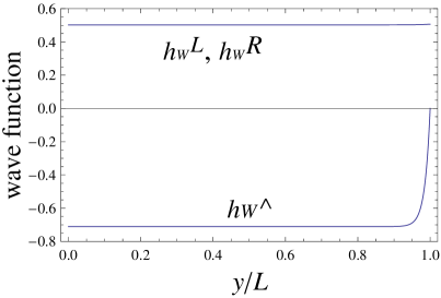
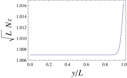
Behavior of the wave functions with respect to $y/L$ is shown in Fig. 1. The wave function of the $W$ boson is flat in most of the region in the bulk in the RS space, which should be contrasted to the case of models in a flat spacetime. In the right figure, the detailed $y$-dependence of $\sqrt{L}N_{W}$ is depicted. In the region where the wave function is flat, $\sqrt{L}N_{W}\simeq 1.00533$. $\sqrt{L}D_{W}\simeq 1-z^{2}/z_{L}^{2}$ for $z/z_{L}\ll 1$.

Figure 1: The $y$-dependence of the wave functions $h_{W}^{L}$, $h_{W}^{R}$ and $h_{W}^{\wedge}$ of the $W$ boson. Here $z_{L}=10^{15}$, $k=4.7\times 10^{17}$ GeV, $m_{W}=80.398$ GeV, $\theta_{H}=\pi/2$.

(ii) Photon tower

The wave functions of the $A_{\mu}^{\gamma}$ bosons in the photon tower are given by

$$h_{\gamma}=cs_{\phi}C(z;\lambda),\qquad h_{\gamma}^{B}=cc_{\phi}C(z;\lambda)$$ (4.15)

where the coefficient $c$ is determined by the normalization $\int_{1}^{z_{L}}dz\,(kz)^{-1}(2(h_{\gamma})^{2}+(h_{\gamma}^{B})^{2})=1$. The mass spectrum is determined by

$$C^{\prime}(1;\lambda)=0.$$ (4.16)

The lowest mass mode is the massless photon. Its wave functions are constant;

$$h_{\gamma}={s_{\phi}\over\sqrt{(1+s_{\phi}^{2})L}},\qquad h_{\gamma}^{B}={c_{\phi}\over\sqrt{(1+s_{\phi}^{2})L}}.$$ (4.17)

It follows from $g_{A}h_{\gamma}(T^{3_{L}}+T^{3_{R}})+g_{B}Q_{X}h_{\gamma}^{B}=Q_{E}g_{A}g_{B}/\sqrt{(g_{A}^{2}+2g_{B}^{2})L}$ that the 4D gauge couplings for weak and electromagnetic interactions are

$${\bar{g}_{A}}={g_{A}\over\sqrt{L}}~{},\qquad e={g_{A}g_{B}\over\sqrt{(g_{A}^{2}+2g_{B}^{2})L}}~{},$$ (4.18)

which lead to $e={\bar{g}_{A}}s_{\phi}/\sqrt{1+s_{\phi}^{2}}$ and $s_{\phi}^{2}=\tan^{2}\theta_{W}$ where $\theta_{W}$ is the weak mixing angle.

(iii) $Z$ boson tower

The wave functions of the bosons in the $Z$ boson tower are

$$\begin{pmatrix}h_{Z}^{L}\cr h_{Z}^{R}\end{pmatrix} \!\!\!=\!\!\! \frac{c_{\phi}^{2}\pm\cos\theta_{H}(1+s_{\phi}^{2})}{2\sqrt{1+s_{\phi}^{2}}}~{}N_{Z}(z;\lambda)~{},$$ (4.19)

$$h_{Z}^{\wedge}~{}~{} \!\!\!=\!\!\! {-\frac{1}{\sqrt{2}}\sin\theta_{H}\sqrt{1+s_{\phi}^{2}}~{}D_{Z}(z;\lambda)}~{},$$ (4.20)

$$h_{Z}^{B}~{}~{} \!\!\!=\!\!\! {-\frac{s_{\phi}c_{\phi}}{\sqrt{1+s_{\phi}^{2}}}~{}N_{Z}(z;\lambda)}~{}.$$ (4.21)

Here $N_{Z}=2b\sqrt{1+s_{\phi}^{2}}C(z;\lambda)$ and $D_{Z}=2b\sqrt{1+s_{\phi}^{2}}(C(1;\lambda)/S(1;\lambda))S(z;\lambda)$. From the normalization condition $\int_{1}^{z_{L}}dz\,(kz)^{-1}\{(h_{Z}^{L})^{2}+(h_{Z}^{R})^{2}+(h_{Z}^{\wedge})^{2}+(h_{Z}^{B})^{2}\}=1$ the coefficient $b$ is determined to be

$$\hskip-28.45274ptb^{-2}=\int_{1}^{z_{L}}\frac{dz}{kz}\,2(1+s_{\phi}^{2})^{2}$$ (4.22)

$$\hskip-14.22636pt\times\Bigg{\{}\frac{2}{1+s_{\phi}^{2}}\,(C(z;\lambda))^{2}-\sin^{2}\theta_{H}\bigg{[}C(z;\lambda)^{2}-\bigg{(}\frac{C(1;\lambda)}{S(1;\lambda)}\bigg{)}^{2}S(z;\lambda)^{2}\bigg{]}\Bigg{\}}~{}.$$ (4.23)

The mass spectrum of the $Z$ tower is determined by

$$2S(1;\lambda)C^{\prime}(1;\lambda)+\lambda(1+s_{\phi}^{2})\sin^{2}\theta_{H}=0~{}.$$ (4.24)

The mass of the lightest mode, the $Z$ boson, is given by

$$m_{Z}\approx{m_{W}\over\cos\theta_{W}}~{}.$$ (4.25)

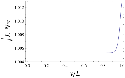
The profile of the wave functions of the $Z$ boson is similar to that of the $W$ boson up to overall factors. The dominant contribution to the normalization comes from $N_{Z}=2b\sqrt{1+s_{\phi}^{2}}C(z;\lambda)$. The figure 2 depicts the $y$-dependence of $\sqrt{L}N_{Z}$ of the $Z$ boson. $\sqrt{L}N_{Z}\simeq 1.00699$ in the region where the wave function is flat. $\sqrt{L}D_{Z}\simeq 1-z^{2}/z_{L}^{2}$ for $z/z_{L}\ll 1$.

Figure 2: The $y$-dependence of $\sqrt{L}N_{Z}$ for the $Z$ boson. Here $z_{L}=10^{15}$, $k=4.7\times 10^{17}$ GeV, $m_{Z}=91.1876$ GeV an d $\theta_{H}=\pi/2$.

4.2 Fermions

In terms of the rescaled fields $\tilde{\Psi}_{a}=z^{-2}\Omega(z)\Psi_{a}$ in the twisted gauge where

$$\Omega(z)=\begin{pmatrix}{\bf 1}_{3}&&\cr&\cos\theta(z)&\sin\theta(z)\cr&-\sin\theta(z)&\cos\theta(z)\end{pmatrix}~{}~{},~{}~{}\theta(z)=\frac{z_{L}^{2}-z^{2}}{z_{L}^{2}-1}\,\theta_{H}~{}~{},$$ (4.26)

the action for the fermions in the bulk region becomes

$$\hskip-28.45274ptS_{\rm bulk}^{\rm fermion}=\sum_{a}\int d^{4}x\frac{dz}{k}~{}i{\overline{\tilde{\Psi}}}_{a}\Big{\{}\Gamma^{\mu}(\partial_{\mu}-ig_{A}\tilde{A}_{\mu}-ig_{B}Q_{Xa}\tilde{B}_{\mu})$$ (4.27)

$$\hskip 22.76228pt+\Gamma^{5}\sigma^{\prime}(\partial_{z}-ig_{A}\tilde{A}_{z}-ig_{B}Q_{Xa}\tilde{B}_{z})-\frac{c_{a}}{z}\,\sigma^{\prime}\Big{\}}~{}\tilde{\Psi}_{a}~{}~{}.$$ (4.28)

If there were no brane interactions, $\tilde{\Psi}_{a}$ would obey

$$\left\{\left(\begin{array}[]{cc}&\sigma\cdot\partial\\ \bar{\sigma}\cdot\partial&\\ \end{array}\right)-k\left(\begin{array}[]{cc}D_{-}(c_{a})&\\ &D_{+}(c_{a})\\ \end{array}\right)\right\}\left(\begin{array}[]{c}\tilde{\Psi}_{aR}\\ \tilde{\Psi}_{aL}\\ \end{array}\right)=0,$$ (4.35)

where $D_{\pm}(c)=\pm(d/dz)+(c/z)$. Neumann conditions for $\tilde{\Psi}_{R}$ and $\tilde{\Psi}_{L}$ are given by $D_{-}(c)\tilde{\Psi}_{R}=0$ and $D_{+}(c)\tilde{\Psi}_{L}=0$, respectively. The resulting second order differential equations are

$$\left\{\partial^{2}-k^{2}D_{-}(c_{a})D_{+}(c_{a})\right\}\tilde{\Psi}_{aL}=0~{},\quad\left\{\partial^{2}-k^{2}D_{+}(c_{a})D_{-}(c_{a})\right\}\tilde{\Psi}_{aR}=0~{}.$$ (4.36)

The basis functions are given by

$$\hskip-28.45274pt\begin{pmatrix}C_{L}\cr S_{L}\end{pmatrix}(z;\lambda,c)=\pm\frac{\pi}{2}\lambda\sqrt{zz_{L}}F_{c+{1\over 2},c\mp{1\over 2}}(\lambda z,\lambda z_{L})~{},$$ (4.37)

$$\hskip-28.45274pt\begin{pmatrix}C_{R}\cr S_{R}\end{pmatrix}(z;\lambda,c)=\mp\frac{\pi}{2}\lambda\sqrt{zz_{L}}F_{c-{1\over 2},c\pm{1\over 2}}(\lambda z,\lambda z_{L})~{}.$$ (4.38)

They satisfy

$$\hskip-28.45274pt\big{\{}D_{+}(c)D_{-}(c)-\lambda^{2}\big{\}}\begin{pmatrix}C_{R}(z)\cr S_{R}(z)\end{pmatrix}=0~{},$$ (4.39)

$$\hskip-28.45274pt\big{\{}D_{-}(c)D_{+}(c)-\lambda^{2}\big{\}}\begin{pmatrix}C_{L}(z)\cr S_{L}(z)\end{pmatrix}=0~{},$$ (4.40)

$$\hskip-28.45274ptS_{L}(z;\lambda,-c)=-S_{R}(z;\lambda,c)~{}~{},~{}~{}C_{L}C_{R}-S_{L}S_{R}=1~{}.$$ (4.41)

They obey the boundary conditions that $C_{R}=C_{L}=1$, $D_{-}C_{R}=D_{+}C_{L}=0$, $S_{R}=S_{L}=0$ and $D_{-}S_{R}=D_{+}S_{L}=\lambda$ at $z=z_{L}$. Further the operators $D_{\pm}$ link $L$ and $R$ functions by $D_{+}(C_{L},S_{L})=\lambda(S_{R},C_{R})$ and $D_{-}(C_{R},S_{R})=\lambda(S_{L},C_{L})$.

(i) Top quark

The wave functions of fermions have been determined in ref. [14]. In the quark sector we choose $c_{1}=c_{2}=c$. The top quark component $t(x)$ in four dimensions is contained in the form

$$\left(\begin{array}[]{c}\tilde{U}_{L}\\ (\tilde{B}_{L}\pm\tilde{t}_{L})/\sqrt{2}\\ \tilde{t}_{L}^{\prime}\\ \end{array}\right)(x,z) \!\!\!=\!\!\! \sqrt{k}\left(\begin{array}[]{c}a_{U}C_{L}(z;\lambda,c)\\ a_{B\pm t}C_{L}(z;\lambda,c)\\ a_{t^{\prime}}S_{L}(z;\lambda,c)\\ \end{array}\right)t_{L}(x),$$ (4.48)

$$\left(\begin{array}[]{c}\tilde{U}_{R}\\ (\tilde{B}_{R}\pm\tilde{t}_{R})/\sqrt{2}\\ \tilde{t}_{R}^{\prime}\\ \end{array}\right)(x,z) \!\!\!=\!\!\! \sqrt{k}\left(\begin{array}[]{c}a_{U}S_{R}(z;\lambda,c)\\ a_{B\pm t}S_{R}(z;\lambda,c)\\ a_{t^{\prime}}C_{R}(z;\lambda,c)\\ \end{array}\right)t_{R}(x).$$ (4.55)

For the right-handed components there are tiny mixture of the brane fermions $\hat{\chi}_{R}$. Their contributions have been shown to be negligibly small.[14] The $u$ and $c$ quarks are described in a similar way. We suppose that the scale of brane masses is much larger than the KK mass scale; $\mu_{1}^{2},\mu_{2}^{2},\mu_{3}^{2},\tilde{\mu}^{2}\gg m_{\rm KK}$. Then the ratios of the coefficients $a$’s are given by

$$[a_{U},a_{B-t},a_{t^{\prime}}]\simeq\left[-{\sqrt{2}\tilde{\mu}\over\mu_{2}},-c_{H},-\frac{s_{H}C_{L}|_{z=1}}{S_{L}|_{z=1}}\right]a_{B+t}~{}~{}.$$ (4.56)

Here $c_{H}=\cos\theta_{H}$ and $s_{H}=\sin\theta_{H}$. The coefficient $a_{B+t}$ is determined by

$$a_{B+t}^{-2}=\int_{1}^{z_{L}}dz\left\{\left(2\left({\tilde{\mu}\over\mu_{2}}\right)^{2}+1+c_{H}^{2}\right)(C_{L}(z))^{2}+s_{H}^{2}\left({C_{L}|_{z=1}\over S_{L}|_{z=1}}\right)^{2}(S_{L}(z))^{2}\right\}.$$ (4.57)

The top quark mass $m_{t}=k\lambda_{t}$ obeys

$$\tilde{\mu}^{2}S_{R}C_{L}+\mu_{2}^{2}C_{L}\left\{S_{R}+{s_{H}^{2}\over 2S_{L}}\right\}\bigg{|}_{z=1,\lambda=\lambda_{t}}=0.$$ (4.58)

This equation contains only the ratio $\tilde{\mu}/\mu_{2}$ and $c$ as parameters. As we will see below, there is the corresponding equation for the bottom quark mass $m_{b}$ which contains the same parameters. A typical set of parameters and the corresponding quark masses are shown in Table 3. The masses of quarks in Table 3 correspond to the central values in the Particle Data Group review. [39] (The analysis with the running masses of quarks and leptons at the $m_{Z}$ scale is given in Appendix D.)

Table 3: The quark and lepton masses are input parameters, from which $c$, $|\tilde{\mu}/\mu_{2}|$ ($|\mu_{3}^{\ell}/\tilde{\mu}^{\ell}|$), and the coefficients of the wave functions are determined. Here $z_{L}=10^{15}$, $k=4.7\times 10^{17}$, $\theta_{H}={\pi\over 2}$ and $\sin^{2}\theta_{W}=0.2312$ which is $\overline{\textrm{MS}}$ value in the ref. [39].

	$c$	$|\tilde{\mu}/\mu_{2}|$, $|\mu_{3}^{\ell}/\tilde{\mu}^{\ell}|$	Mass (GeV)
$W$,$Z$			80.398	91.1876
$u$,$d$	0.8277	1.979	$2.4\times 10^{-3}$	$4.75\times 10^{-3}$
$c$,$s$	0.6564	0.08189	1.27	0.104
$t$,$b$	0.4329	0.02513	171.2	4.20
$\nu_{e}$,$e$	0.8992	$5.110\times 10^{8}$	$10^{-12}$	$0.510998910\times 10^{-3}$
$\nu_{\mu}$,$\mu$	0.7354	$1.174\times 10^{10}$	$9\times 10^{-12}$	0.105658367
$\nu_{\tau}$,$\tau$	0.6456	$3.532\times 10^{10}$	$5.0309\times 10^{-11}$	1.77684

	$a_{U}$	$a_{B+t}$	$a_{t^{\prime}}$
$u$	$-2.774\times 10^{-13}$	$9.909\times 10^{-14}$	$5.153\times 10^{-8}$
$c$	$-6.507\times 10^{-12}$	$5.619\times 10^{-11}$	$4.809\times 10^{-8}$
$t$	$-3.102\times 10^{-10}$	$8.728\times 10^{-9}$	$4.388\times 10^{-8}$
	$a_{b}$	$a_{D+X}$	$a_{b^{\prime}}$
$d$	$-1.401\times 10^{-13}$	$1.961\times 10^{-13}$	$-5.153\times 10^{-8}$
$s$	$-7.946\times 10^{-11}$	$4.601\times 10^{-12}$	$-4.809\times 10^{-8}$
$b$	$-1.164\times 10^{-8}$	$2.069\times 10^{-10}$	$-4.319\times 10^{-8}$
	$a_{\nu_{\tau}}$	$a_{L_{2Y}+L_{3X}}$	$a_{\nu^{\prime}_{\tau}}$
$\nu_{e}$	$-2.907\times 10^{-14}$	$4.022\times 10^{-23}$	$5.290\times 10^{-8}$
$\nu_{\mu}$	$-6.396\times 10^{-12}$	$3.852\times 10^{-22}$	$4.971\times 10^{-8}$
$\nu_{\tau}$	$-1.117\times 10^{-10}$	$2.236\times 10^{-21}$	$4.787\times 10^{-8}$
	$a_{L_{3Y}}$	$a_{\tau+L_{1X}}$	$a_{\tau^{\prime}}$
$e$	$-8.662\times 10^{-22}$	$2.055\times 10^{-14}$	$-5.290\times 10^{-8}$
$\mu$	$-3.566\times 10^{-19}$	$4.523\times 10^{-12}$	$-4.971\times 10^{-8}$
$\tau$	$-5.520\times 10^{-18}$	$7.898\times 10^{-11}$	$-4.787\times 10^{-8}$

(ii) Bottom quark

The bottom quark component $b(x)$ is contained in the form

$$\left(\begin{array}[]{c}\tilde{b}_{L}\\ {1\over\sqrt{2}}(\tilde{D}_{L}\pm\tilde{X}_{L})\\ \tilde{b}_{L}^{\prime}\\ \end{array}\right)(x,z) \!\!\!=\!\!\! \sqrt{k}\left(\begin{array}[]{c}a_{b}C_{L}(z;\lambda,{c})\\ a_{D\pm X}C_{L}(z;\lambda,{c})\\ a_{b^{\prime}}S_{L}(z;\lambda,{c})\\ \end{array}\right)b_{L}(x),$$ (4.65)

$$\left(\begin{array}[]{c}\tilde{b}_{R}\\ {1\over\sqrt{2}}(\tilde{D}_{R}\pm\tilde{X}_{R})\\ \tilde{b}_{R}^{\prime}\\ \end{array}\right)(x,z) \!\!\!=\!\!\! \sqrt{k}\left(\begin{array}[]{c}a_{b}S_{R}(z;\lambda,{c})\\ a_{D\pm X}S_{R}(z;\lambda,{c})\\ a_{b^{\prime}}C_{R}(z;\lambda,{c})\\ \end{array}\right)b_{R}(x)~{}.$$ (4.72)

The $d$ and $s$ quarks are described in a similar manner. The ratios of the coefficients are given by

$$[a_{b},a_{D-X},a_{b^{\prime}}]\,{\simeq}\left[-{\sqrt{2}\mu_{2}\over\tilde{\mu}},c_{H},{s_{H}C_{L}|_{z=1}\over S_{L}|_{z=1}}\right]a_{D+X}~{}.$$ (4.73)

The coefficient $a_{D+X}$ is given by

$$a_{D+X}^{-2}=\int_{1}^{z_{L}}dz\left\{\left(2\left({\mu_{2}\over\tilde{\mu}}\right)^{2}+1+c_{H}^{2}\right)(C_{L}(z))^{2}+s_{H}^{2}\left({C_{L}|_{z=1}\over S_{L}|_{z=1}}\right)^{2}(S_{L}(z))^{2}\right\}.$$ (4.74)

The mass $m_{b}=k\lambda_{b}$ obeys

$$\mu_{2}^{2}S_{R}C_{L}+\tilde{\mu}^{2}C_{L}\left\{S_{R}+{s_{H}^{2}\over 2S_{L}}\right\}\bigg{|}_{z=1,\lambda=\lambda_{b}}=0.$$ (4.75)

Combining Eqs. (4.58) and (4.75), one finds

$$\frac{\tilde{\mu}^{2}}{\mu_{2}^{2}} \!\!\!=\!\!\! -\bigg{\{}1+\frac{s_{H}^{2}}{2S_{L}(1;\lambda_{t},c)S_{R}(1;\lambda_{t},c)}\bigg{\}}$$ (4.76)

$$\!\!\!=\!\!\! -\bigg{\{}1+\frac{s_{H}^{2}}{2S_{L}(1;\lambda_{b},c)S_{R}(1;\lambda_{b},c)}\bigg{\}}^{-1}~{}.$$ (4.77)

The value of $\theta_{H}$ is dynamically determined.[4, 5, 40, 41] In the present model the contributions to the effective potential $V_{\rm eff}(\theta_{H})$ from multiplets containing the top quark dominate, whereas the contributions from other quarks and leptons are negligible. $V_{\rm eff}(\theta_{H})$ has global minima at $\theta_{H}=\pm\hbox{${1\over 2}$}\pi$.[13] Hence, given $k$ (or $z_{L}$) , $m_{t}$, $m_{b}$, the parameters $c$ and $|\tilde{\mu}/\mu_{2}|$ are determined. These values are not sensitive on the value of $k$ very much. See Table 3.

The wave functions $C_{L}$ and $S_{L}$ for the left-handed quarks $t_{L}$, $b_{L}$ are localized near the Planck brane, whereas $C_{R}$ and $S_{R}$ for the right-handed quarks $t_{R}$, $b_{R}$ are localized near the TeV brane.

Generalization to the case of three generations of quarks is straightforward. If there were no flavor mixing, it would be enough to replace $(\lambda_{t},\lambda_{b})$ in the above formulas by $(\lambda_{c},\lambda_{s})$ or $(\lambda_{u},\lambda_{d})$ to determine the wave functions of $(c,s)$ of $(u,d)$ quarks, respectively. The flavor mass mixing is incorporated by considering 3-by-3 matrices for $\mu_{2}$ and $\tilde{\mu}$, in which case the formulas become more involved. In the present paper we evaluate electroweak gauge couplings with the mixing turned off.

(iii) Leptons

We need to introduce only a vector multiplet $\Psi_{3}$ in Table 2 to describe a massless neutrino for each generation. The $\tau$ lepton is contained in the form

$$\left(\begin{array}[]{c}{1\over\sqrt{2}}(\tilde{\tau}_{L}\pm\tilde{L}_{1XL})\\ \tilde{\tau}_{L}^{\prime}\\ \end{array}\right)(x,z) \!\!\!=\!\!\! \sqrt{k}\left(\begin{array}[]{c}a_{\tau\pm L_{1X}}C_{L}(z;\lambda,c_{3})\\ a_{\tau^{\prime}}S_{L}(z;\lambda,c_{3})\\ \end{array}\right)\tau_{L}(x)~{},$$ (4.82)

$$\left(\begin{array}[]{c}{1\over\sqrt{2}}(\tilde{\tau}_{R}\pm\tilde{L}_{1XR})\\ \tilde{\tau}_{R}^{\prime}\\ \end{array}\right)(x,z) \!\!\!=\!\!\! \sqrt{k}\left(\begin{array}[]{c}a_{\tau\pm L_{1X}}S_{R}(z;\lambda,c_{3})\\ a_{\tau^{\prime}}C_{R}(z;\lambda,c_{3})\\ \end{array}\right)\tau_{R}(x)~{}.$$ (4.87)

$e,\mu$ leptons are described in a similar way. The ratios of the coefficients are given by

$$[a_{\tau-L_{1X}},a_{\tau^{\prime}}]\simeq\left[c_{H},{s_{H}C_{L}|_{z=1}\over S_{L}|_{z=1}}\right]a_{\tau+L_{1X}},$$ (4.88)

for $(\mu_{1}^{\ell})^{2}\gg m_{\rm KK}$. The coefficient $a_{\tau+L_{1X}}$ is given by

$$a_{\tau+L_{1X}}^{-2}=\int_{1}^{z_{L}}dz\left\{\left(1+c_{H}^{2}\right)(C_{L}(z))^{2}+s_{H}^{2}\left({C_{L}|_{z=1}\over S_{L}|_{z=1}}\right)^{2}(S_{L}(z))^{2}\right\}.$$ (4.89)

The mass $m_{\tau}=k\lambda_{\tau}$ is determined by

$$(\mu_{1}^{\ell})^{2}C_{L}\left\{S_{R}+{s_{H}^{2}\over 2S_{L}}\right\}\bigg{|}_{z=1}=0.$$ (4.90)

To describe massive neutrinos one needs to introduce two multiplets $\Psi_{3}$ and $\Psi_{4}$. The structure is the same as in the quark sector. Take $c_{3}=c_{4}\equiv c$. The left-handed components are contained in the form

$$\left(\begin{array}[]{c}\tilde{\nu}_{\tau L}\\ {1\over\sqrt{2}}(\tilde{L}_{2YL}\pm\tilde{L}_{3XL})\\ \tilde{\nu}^{\prime}_{\tau L}\\ \end{array}\right)(x,z) \!\!\!=\!\!\! \sqrt{k}\left(\begin{array}[]{c}a_{\nu_{\tau}}C_{L}(z;\lambda,c)\\ a_{L_{2Y}\pm L_{3X}}C_{L}(z;\lambda,c)\\ a_{\nu^{\prime}_{\tau}}S_{L}(z;\lambda,c)\\ \end{array}\right)\nu_{\tau L}(x),$$ (4.97)

$$\left(\begin{array}[]{c}\tilde{L}_{3YL}\\ {1\over\sqrt{2}}(\tilde{\tau}_{L}\pm\tilde{L}_{1XL})\\ \tilde{\tau}^{\prime}_{L}\\ \end{array}\right)(x,z) \!\!\!=\!\!\! \sqrt{k}\left(\begin{array}[]{c}a_{L_{3Y}}C_{L}(z;\lambda,c)\\ a_{\tau\pm L_{1X}}C_{L}(z;\lambda,c)\\ a_{\tau^{\prime}}S_{L}(z;\lambda,c)\\ \end{array}\right)\tau_{L}(x)~{}.$$ (4.104)

The right-handed components have the same form as in Eq. (4.104) with $(C_{L},S_{L})$ replaced by $(S_{R},C_{R})$. The equations of motion for leptons are obtained by employing the correspondence between leptons and quarks: $(\nu_{\tau},L_{2Y},L_{3X},\nu^{\prime}_{\tau}$, $\hat{L}_{3XR},\hat{L}_{2YR})\leftrightarrow(U,B,t,t^{\prime}$, $\hat{U}_{R},\hat{B}_{R})$ for $T^{3_{L}}=+1/2$, $(L_{3YL},\tau,L_{1X},\tau^{\prime}$, $\hat{L}_{3YR},\hat{L}_{1XR})\leftrightarrow(b,D,X,b^{\prime}$, $\hat{D}_{R},\hat{X}_{R})$ for $T^{3_{L}}=-1/2$ and $(\mu_{1}^{\ell},\mu_{2}^{\ell},\mu_{3}^{\ell},\tilde{\mu}^{\ell})\leftrightarrow(\mu_{3},\mu_{1},\tilde{\mu},\mu_{2})$. Similarly to Eq. (4.77), the ratio of the couplings is given by

$$\frac{(\mu_{3}^{\ell})^{2}}{(\tilde{\mu}^{\ell})^{2}} \!\!\!=\!\!\! -\bigg{\{}1+\frac{s_{H}^{2}}{2S_{L}(1;\lambda_{\nu_{\tau}},c)S_{R}(1;\lambda_{\nu_{\tau}},c)}\bigg{\}}$$ (4.105)

$$\!\!\!=\!\!\! -\bigg{\{}1+\frac{s_{H}^{2}}{2S_{L}(1;\lambda_{\tau},c)S_{R}(1;\lambda_{\tau},c)}\bigg{\}}^{-1}~{}.$$ (4.106)

As in the quark sector, generalization to three generations of leptons is straightforward. The flavor mixing is incorporated by taking 3-by-3 matrices for $\mu_{2}^{\ell}$ and $\tilde{\mu}^{\ell}$. The observed mixing in the neutrino sector is large. In the present paper we content ourselves with considering the diagonal flavor. The wave functions of the real neutrinos would change in the flavor space significantly, but the effect to the gauge couplings of charged leptons would be small provided that all neutrino masses are much smaller than the masses of charged leptons.

Table 3 includes $c$ and $|\mu_{3}^{\ell}/\tilde{\mu}^{\ell}|$ for leptons in the diagonal flavor case. For neutrinos, the values $m_{\nu_{e}}=10^{-3}$eV and $(m_{\nu_{e}},m_{\nu_{\mu}},m_{\nu_{\tau}})=(m_{\nu_{1}},m_{\nu_{2}},m_{\nu_{3}})$ are taken. The input parameters correspond to the values derived from the mass squared differences $\Delta m_{21}^{2}=8\times 10^{-5}\textrm{eV}^{2}$, $\Delta m_{32}^{2}=2.45\times 10^{-3}\textrm{eV}^{2}$ which are the central values quoted in ref. [39]. The case $\Delta m_{32}^{2}=-2.45\times 10^{-3}\textrm{eV}^{2}$ can be analysed similarly. The masses of charged leptons correspond to the central values in ref. [39].

To compare various predictions with experiments, one needs to use the running masses of quarks and leptons at the typical energy scale of the problem under consideration. Results obtained with the input of running masses of quarks and leptons at the $m_{Z}$ scale are summarized in Appendix D. It is found that the coefficients of mode functions and the resulting gauge couplings are not very sensitive to the choice of these input parameters.

As in ref. [14], we define the normalized coefficients $a_{j}^{\prime L,R}$ by

$$(a_{U}^{\prime L},a_{B\pm t}^{\prime L},a_{t^{\prime}}^{\prime L}) \!\!\!=\!\!\! (\sqrt{N_{C_{L}}}a_{U},\sqrt{N_{C_{L}}}a_{B\pm t},\sqrt{N_{S_{L}}}a_{t^{\prime}}),$$

$$(a_{U}^{\prime R},a_{B\pm t}^{\prime R},a_{t^{\prime}}^{\prime R}) \!\!\!=\!\!\! (\sqrt{N_{S_{R}}}a_{U},\sqrt{N_{S_{R}}}a_{B\pm t},\sqrt{N_{C_{R}}}a_{t^{\prime}}),$$ (4.107)

where $N_{C_{L}}=\int_{1}^{z_{L}}dzC_{L}(z;\lambda,c)^{2}$, etc. These coefficients satisfy $|a^{\prime L}_{U}|^{2}+|a^{\prime L}_{B+t}|^{2}+|a^{\prime L}_{B-t}|^{2}+|a^{\prime L}_{t^{\prime}}|^{2}=1$ etc. so that $|a^{\prime L,R}_{j}|^{2}$ represents the weight of the $j$-th component in each quark or lepton. They are tabulated in Table 4 and Table 5. At $\theta_{H}=\hbox{${1\over 2}$}\pi$, all of the $a^{\prime}_{B-t}$, $a^{\prime}_{D-X}$, $a^{\prime}_{L_{1Y}-L_{2X}}$, and $a^{\prime}_{\tau-L_{1X}}$ components vanish.

Table 4: Normalized coefficients in mode expansion for quarks.

	$a^{\prime}_{UL}$	$a^{\prime}_{B+t\,L}$	$a^{\prime}_{t^{\prime}L}$	$a^{\prime}_{UR}$	$a^{\prime}_{B+t\,R}$	$a^{\prime}_{t^{\prime}R}$
$u$	$-0.8925$	0.3189	0.3189	$-2.370\times 10^{-11}$	$8.468\times 10^{-12}$	1
$c$	$-0.08162$	0.7047	0.7047	$-2.815\times 10^{-7}$	$2.430\times 10^{-6}$	1
$t$	$-0.02582$	0.7265	0.6867	$-0.001769$	0.04976	0.9988
	$a^{\prime}_{bL}$	$a^{\prime}_{D+XL}$	$a^{\prime}_{b^{\prime}L}$	$a^{\prime}_{bR}$	$a^{\prime}_{D+XR}$	$a^{\prime}_{b^{\prime}R}$
$d$	$-0.4510$	0.6311	$-0.6311$	$-2.370\times 10^{-11}$	$3.317\times 10^{-11}$	$-1$
$s$	$-0.9967$	0.05771	$-0.05771$	$-2.815\times 10^{-7}$	$1.630\times 10^{-8}$	$-1$
$b$	$-0.9997$	0.01777	$-0.01685$	$-0.001648$	0.00002930	$-1$

Table 5: Normalized coefficients in mode expansion for leptons.

	$a^{\prime}_{\nu_{\tau}L}$	$a^{\prime}_{L_{2Y}+L_{3X}L}$	$a^{\prime}_{\nu^{\prime}_{\tau}L}$	$a^{\prime}_{\nu_{\tau}R}$	$a^{\prime}_{L_{2Y}+L_{3X}R}$	$a^{\prime}_{\nu^{\prime}_{\tau}R}$
$\nu_{e}$	$-1$	$1.384\times\!\!10^{-9}$	$1.384\times\!\!10^{-9}$	$-1.066\times\!\!10^{-21}$	$1.476\times\!\!10^{-30}$	1
$\nu_{\mu}$	$-1$	$6.023\times\!\!10^{-11}$	$6.023\times\!\!10^{-11}$	$-1.993\times\!\!10^{-18}$	$1.200\times\!\!10^{-28}$	1
$\nu_{\tau}$	$-1$	$2.002\times\!\!10^{-11}$	$2.002\times\!\!10^{-11}$	$-1.911\times\!\!10^{-16}$	$3.825\times\!\!10^{-27}$	1
	$a^{\prime}_{L_{3Y}L}$	$a^{\prime}_{\tau+L_{1X}L}$	$a^{\prime}_{\tau^{\prime}L}$	$a^{\prime}_{L_{3Y}R}$	$a^{\prime}_{\tau+L_{1X}R}$	$a^{\prime}_{\tau^{\prime}R}$
$e$	$-2.980\times\!\!10^{-8}$	0.7071	$-0.7071$	$-1.624\times\!\!10^{-20}$	$3.853\times\!\!10^{-13}$	$-1$
$\mu$	$-5.576\times\!\!10^{-8}$	0.7071	$-0.7071$	$-1.304\times\!\!10^{-15}$	$1.654\times\!\!10^{-8}$	$-1$
$\tau$	$-4.942\times\!\!10^{-8}$	0.7071	$-0.7071$	$-3.335\times\!\!10^{-13}$	$4.772\times\!\!10^{-6}$	$-1$

The left-handed quarks have contributions from both singlet and non-singlet components of $SU(2)_{L}\times SU(2)_{R}$. The left-handed neutrinos have contributions almost entirely from the $T^{3_{L}}=T^{3_{R}}=+1/2$ component. The left-handed charged leptons receive contributions from the $T^{3_{L}}=-T^{3_{R}}=\pm 1/2$ component and the singlet component. The right-handed quarks and leptons are dominated by the singlet component.

Regarding the isospin eigenvalues in $SU(2)_{L}\times SU(2)_{R}$, all the nonvanishing components are found to be left-right symmetric. Indeed the eigenvalues are given by $T^{3_{L}}=T^{3_{R}}=+1/2$ for $(U,\nu_{\tau})$, $T^{3_{L}}=T^{3_{R}}=-1/2$ for $(b,L_{3Y})$, $T^{3_{L}}=T^{3_{R}}=0$ for $(t^{\prime},b^{\prime},\nu^{\prime}_{\tau},\tau^{\prime})$ and $(T^{3_{L}}=-T^{3_{R}}=+1/2)\oplus(T^{3_{L}}=-T^{3_{R}}=-1/2)$ for $(B+t,D+X,L_{2Y}+L_{3X},\tau+L_{1X})$. The left-right symmetry is preserved as the left-right antisymmetric part vanishes at $\theta_{H}=\pm\pi/2$. As expected from the situation in the left-right symmetric models, we will see in the next section that the gauge couplings deviate little from those in the standard model.

5 Electroweak currents

Inserting the wave functions of the 4D gauge fields $A_{\mu}^{\gamma}(x)$, $W_{\mu}(x)$ and $Z_{\mu}(x)$ into the 5D gauge couplings, one finds that

$$\hskip-28.45274ptg_{A}\tilde{A}_{\mu}(x,z)+g_{B}Q_{X}\tilde{B}_{\mu}(x,z)=eA_{\mu}^{\gamma}(x)Q_{E}$$ (5.1)

$$\hskip 14.22636pt+g_{A}W_{\mu}(x)\bigg{\{}N_{W}(z)T^{-}(\theta_{H})-D_{W}(z)\frac{\sin\theta_{H}}{\sqrt{2}}T^{\hat{-}}\bigg{\}}$$ (5.2)

$$\hskip 14.22636pt+g_{A}W_{\mu}^{\dagger}(x)\bigg{\{}N_{W}(z)T^{+}(\theta_{H})-D_{W}(z)\frac{\sin\theta_{H}}{\sqrt{2}}T^{\hat{+}}\bigg{\}}$$ (5.3)

$$\hskip 14.22636pt+\frac{g_{A}Z_{\mu}(x)}{\cos\theta_{W}}\bigg{\{}N_{Z}(z)\Big{(}T^{3}(\theta_{H})-\sin^{2}\theta_{W}\,Q_{E}\Big{)}-D_{Z}(z)\frac{\sin\theta_{H}}{\sqrt{2}}T^{\hat{3}}\bigg{\}}~{},$$ (5.4)

$$\hskip-28.45274ptT^{a}(\theta_{H})=\frac{1+\cos\theta_{H}}{2}T^{a_{L}}+\frac{1-\cos\theta_{H}}{2}T^{a_{R}}~{},~{}~{}T^{\pm}=\frac{T^{1}\pm iT^{2}}{\sqrt{2}}~{}.$$ (5.5)

The wave functions $N_{W,Z}(z)$ and $D_{W,Z}(z)$ have been defined in the previous section. Explicit forms of gauge couplings with fermions in the vector representation of $SO(5)$ are given in Appendix B. The observed weak $SU(2)$ is the mixture of the original $SU(2)_{L}$ and $SU(2)_{R}$. There appear $T^{\hat{a}}$ components as well.

4D gauge couplings of quarks and leptons are obtained by inserting their wave functions into $\tilde{\Psi}_{a}(x,z)$ and integrating

$$\sum_{a}\int_{1}^{z_{L}}\frac{dz}{k}\,\overline{\tilde{\Psi}}_{a}\Gamma^{\mu}(g_{A}\tilde{A}_{\mu}+g_{B}Q_{Xa}\tilde{B}_{\mu})\tilde{\Psi}_{a}~{}.$$

in (4.28). As they appear as overlap integrals, the 4D gauge couplings are not universal and are expected to deviate from those in the standard model at nonvanishing $\theta_{H}$. Surprisingly the deviation turns out very small, although the wave functions have significant dependence on $\theta_{H}$. Useful formulas for evaluating 4D gauge-fermion couplings are given in Appendix C.

(i) Photon couplings

The photon couplings are universal. The $U(1)_{\rm EM}$ invariance remains intact. The wave function of the photon is constant with respect to $z$ so that the $z$-integrals for the gauge couplings are fixed by the normalization of the fermion wave functions. For the third generation one finds that

$$eA_{\mu}^{\gamma}\bigg{\{}{2\over 3}(\bar{t}_{L}\gamma^{\mu}t_{L}+\bar{t}_{R}\gamma^{\mu}t_{R})-{1\over 3}(\bar{b}_{L}\gamma^{\mu}b_{L}+\bar{b}_{R}\gamma^{\mu}b_{R})-(\bar{\tau}_{L}\gamma^{\mu}\tau_{L}+\bar{\tau}_{R}\gamma^{\mu}\tau_{R})\bigg{\}}~{}.$$ (5.6)

(ii) $W$ boson couplings

There arise deviations in the $W$ boson couplings from the standard model. For the $t$ and $b$ quarks their interactions are given by

$${1\over 2}g^{(W)}_{tb,L}(W_{\mu}\bar{b}_{L}\gamma^{\mu}t_{L}+W_{\mu}^{\dagger}\bar{t}_{L}\gamma^{\mu}b_{L})+{1\over 2}g^{(W)}_{tb,R}(W_{\mu}\bar{b}_{R}\gamma^{\mu}t_{R}+W_{\mu}^{\dagger}\bar{t}_{R}\gamma^{\mu}b_{R}).$$ (5.7)

Not only left-handed components but also right-handed components couple to $W$ in general. The couplings are given by

$$g^{(W)}_{tb,L} \!\!\!=\!\!\! g_{A}\int_{1}^{z_{L}}dz\,\bigg{[}N_{W}C_{L}(\lambda_{b})C_{L}(\lambda_{t})\Big{\{}(a_{D+X}+a_{D-X})a_{U}+a_{b}(a_{B+t}-a_{B-t})\Big{\}}$$ (5.10)

$$-(1-\cos\theta_{H})N_{W}C_{L}(\lambda_{b})C_{L}(\lambda_{t})(a_{D-X}a_{U}-a_{b}a_{B-t})$$

$$-\sin\theta_{H}D_{W}\Big{\{}C_{L}(\lambda_{b})S_{L}(\lambda_{t})a_{b}a_{t^{\prime}}-S_{L}(\lambda_{b})C_{L}(\lambda_{t})a_{b^{\prime}}a_{U}\Big{\}}\bigg{]}~{}.$$

Here $N_{W}=N_{W}(z)$, $C_{L}(\lambda)=C_{L}(z;\lambda)$ etc. The formula for $g^{(W)}_{tb,R}$ is obtained from (5.10) by replacing $C_{L}(\lambda)$ and $S_{L}(\lambda)$ by $S_{R}(\lambda)$ and $C_{R}(\lambda)$, respectively.

We have tabulated the numerical values of these couplings at $\theta_{H}=\hbox{${1\over 2}$}\pi$ in Table 6. In the table the normalized couplings

$$g^{\prime(W)}_{f,LR}=\frac{1}{{g_{W}}}g^{(W)}_{f,LR}~{}~{},~{}~{}{g_{W}}=g^{(W)}_{e\nu,L}$$ (5.11)

are also listed where $g_{W}$ is the measured $We\nu_{e}$ coupling, corresponding to the $SU(2)_{L}$ coupling in the standard model. The origin of the value $g^{(W)}_{e\nu,L}/\bar{g}_{A}=1.00533$, where $\bar{g}_{A}$ is the 4D gauge coupling defined in (4.18), is traced back to $\sqrt{L}N_{W}\simeq 1.00533$ as described in Section 4.1.

Table 6: The $W$ couplings $g^{(W)}_{f,LR}$ and $g^{\prime(W)}_{f,LR}=g^{(W)}_{f,LR}/{g_{W}}$ at $\theta_{H}=\hbox{${1\over 2}$}\pi$. (${g_{W}}\equiv g^{(W)}_{e\nu L}$.) Here the parameters given in Table 3 are used.

$f$	$u,d$	$c,s$	$t,b$
$g^{(W)}_{fL}/{\bar{g}_{A}}$	1.00533	1.00533	0.98192
$g^{(W)}_{fR}/{\bar{g}_{A}}$	$-1.399\times\!\!10^{-11}$	$-1.906\times\!\!10^{-7}$	$-0.001271$
$g^{\prime(W)}_{fL}$	1.	1.	0.9767
$g^{\prime(W)}_{fR}$	$-1.392\times\!\!10^{-11}$	$-1.896\times\!\!10^{-7}$	$-0.001264$
$f$	$\nu_{e},e$	$\nu_{\mu},\mu$	$\nu_{\tau},\tau$
$g^{(W)}_{fL}/{\bar{g}_{A}}$	1.00533	1.00533	1.00533
$g^{(W)}_{fR}/{\bar{g}_{A}}$	$-4.787\times\!\!10^{-21}$	$-4.163\times\!\!10^{-16}$	$-1.139\times\!\!10^{-13}$
$g^{\prime(W)}_{fL}$	1.	1.	1.
$g^{\prime(W)}_{fR}$	$-4.761\times\!\!10^{-21}$	$-4.141\times\!\!10^{-16}$	$-1.133\times\!\!10^{-13}$

Table 7: The deviation $g^{\prime(W)}_{fL}-1$ of the $W$ couplings from the standard model, which represents the violation of the universality.

	$g^{\prime(W)}_{fL}-1$
$f$	$\nu_{\mu},\mu$	$\nu_{\tau},\tau$	$u,d$	$c,s$	$t,b$
	$-1.022\times\!\!10^{-8}$	$-2.736\times\!\!10^{-6}$	$-2.778\times\!\!10^{-11}$	$-1.415\times\!\!10^{-6}$	$-0.02329$

Notice that the couplings of left-handed quarks and leptons are close to $g_{W}$ except for the top quark. To see the tiny violation of the weak universality we have listed $g^{\prime(W)}_{fL}-1$ in Table 7. By definition, $g^{\prime(W)}_{\nu_{e},e\,L}-1=0$. The violation of the $\mu$-$e$ universality is of $-1.022\times 10^{-8}$ for $z_{L}=10^{15}$, which is below the current limit. Similar behavior has been previously reported in the $SU(3)$ model in ref. [25]. The violation becomes appreciable for the $tb$ coupling. The couplings of right-handed quarks and leptons are nonvanishing, but are all tiny.

(iii) $Z$ boson couplings

The $Z$ boson couplings of $t$ and $b$ quarks take the form

$$\hskip-28.45274pt\frac{1}{\cos\theta_{W}}Z_{\mu}\bigg{\{}g^{(Z)}_{tL}\bar{t}_{L}\gamma^{\mu}t_{L}+g^{(Z)}_{tR}\bar{t}_{R}\gamma^{\mu}t_{R}+g^{(Z)}_{bL}\bar{b}_{L}\gamma^{\mu}b_{L}+g^{(Z)}_{bR}\bar{b}_{R}\gamma^{\mu}b_{R}\bigg{\}},$$ (5.12)

$$\hskip 28.45274ptg^{(Z)}_{tL,R}=+\frac{1}{2}g^{(Z)3}_{tL,R}-\frac{2}{3}g^{(Z)Q}_{tL,R}\sin^{2}\theta_{W}~{},$$ (5.13)

$$\hskip 28.45274ptg^{(Z)}_{bL,R}=-\frac{1}{2}g^{(Z)3}_{bL,R}+\frac{1}{3}g^{(Z)Q}_{bL,R}\sin^{2}\theta_{W}~{}.$$ (5.14)

Here the couplings $g^{(Z)3}$ and $g^{(Z)Q}$ are given by

$$g_{tL}^{(Z)3} \!\!\!=\!\!\! g_{A}\int_{1}^{z_{L}}dz\,\Big{\{}N_{Z}(C_{L}(\lambda_{t}))^{2}\big{(}a_{U}^{2}-2\cos\theta_{H}a_{B+t}a_{B-t}\big{)}$$ (5.16)

$$\hskip 99.58464pt-2\sin\theta_{H}D_{Z}C_{L}(\lambda_{t})S_{L}(\lambda_{t})a_{B+t}a_{t^{\prime}}\Big{\}},$$

$$g_{tL}^{(Z)Q} \!\!\!=\!\!\! g_{A}\int_{1}^{z_{L}}dz\,N_{Z}\Big{\{}(C_{L}(\lambda_{t}))^{2}\big{(}a_{U}^{2}+a_{B+t}^{2}+a_{B-t}^{2}\big{)}+(S_{L}(\lambda_{t}))^{2}a_{t^{\prime}}^{2}\Big{\}},$$ (5.17)

$$g_{bL}^{(Z)3} \!\!\!=\!\!\! g_{A}\int_{1}^{z_{L}}dz\,\Big{\{}N_{Z}(C_{L}(\lambda_{b}))^{2}\big{(}a_{b}^{2}+2\cos\theta_{H}a_{D+X}a_{D-X}\big{)}$$ (5.19)

$$\hskip 99.58464pt+2\sin\theta_{H}D_{Z}C_{L}(\lambda_{b})S_{L}(\lambda_{b})a_{D+X}a_{b^{\prime}}\Big{\}},$$

$$g_{bL}^{(Z)Q} \!\!\!=\!\!\! g_{A}\int_{1}^{z_{L}}dz\,N_{Z}\Big{\{}(C_{L}(\lambda_{b}))^{2}\big{(}a_{b}^{2}+a_{D+X}^{2}+a_{D-X}^{2}\big{)}+(S_{L}(\lambda_{b}))^{2}a_{b^{\prime}}^{2}\Big{\}}.$$ (5.20)

The formulas for $g_{tb,R}^{(Z)3}$ and $g_{tb,R}^{(Z)Q}$ are obtained from (5.20) by replacing $C_{L}(\lambda)$ and $S_{L}(\lambda)$ by $S_{R}(\lambda)$ and $C_{R}(\lambda)$, respectively.

Table 8: $Z$ boson couplings of quarks at $\theta_{H}=\hbox{${1\over 2}$}\pi$. For entry denoted as SM, $g^{(Z)}_{tL}/{\bar{g}_{A}}$ and $g^{(Z)}_{bL}/{\bar{g}_{A}}$ are ${1\over 2}-{2\over 3}\sin^{2}\theta_{W}$ and $-{1\over 2}+{1\over 3}\sin^{2}\theta_{W}$, respectively.

$f$	$u$	$c$	$t$	SM
$g^{(Z)}_{fL}/{\bar{g}_{A}}$	0.3483	0.3483	0.3221	0.3459
$g^{(Z)}_{fR}/{\bar{g}_{A}}$	$-0.1564$	$-0.1564$	$-0.1833$	$-0.1541$
$g^{(Z)3}_{fL}/{\bar{g}_{A}}$	1.00699	1.00698	0.9549	1
$g^{(Z)3}_{fR}/{\bar{g}_{A}}$	$-7.086\times\!\!10^{-12}$	$-2.332\times\!\!10^{-6}$	$-0.05400$	0
$g^{(Z)Q}_{fL}/{\bar{g}_{A}}$	1.00699	1.00699	1.0079	1
$g^{(Z)Q}_{fR}/{\bar{g}_{A}}$	1.0141	1.0145	1.0141	1
$f$	$d$	$s$	$b$	SM
$g^{(Z)}_{fL}/{\bar{g}_{A}}$	$-0.4259$	$-0.4259$	$-0.4264$	$-0.4229$
$g^{(Z)}_{fR}/{\bar{g}_{A}}$	0.07820	0.07818	0.07816	0.07707
$g^{(Z)3}_{fL}/{\bar{g}_{A}}$	1.00699	1.00699	1.00813	1
$g^{(Z)3}_{fR}/{\bar{g}_{A}}$	$-2.776\times\!\!10^{-11}$	$-1.564\times\!\!10^{-8}$	$-0.00003003$	0
$g^{(Z)Q}_{fL}/{\bar{g}_{A}}$	1.00699	1.00699	1.00816	1
$g^{(Z)Q}_{fR}/{\bar{g}_{A}}$	1.0148	1.0145	1.0140	1

Table 9: $Z$ boson couplings of leptons at $\theta_{H}=\hbox{${1\over 2}$}\pi$. For entry denoted as SM, $g^{(Z)}_{\nu_{\tau}L}/{\bar{g}_{A}}$ and $g^{(Z)}_{\tau L}/{\bar{g}_{A}}$ are ${1\over 2}$ and $-{1\over 2}+\sin^{2}\theta_{W}$, respectively.

$f$	$\nu_{e}$	$\nu_{\mu}$	$\nu_{\tau}$	SM
$g^{(Z)}_{fL}/{\bar{g}_{A}}$	0.5035	0.5035	0.5035	0.5
$g^{(Z)}_{fR}/{\bar{g}_{A}}$	$-5.785\times\!\!10^{-31}$	$-5.421\times\!\!10^{-29}$	$-1.850\times\!\!10^{-27}$	$0$
$g^{(Z)3}_{fL}/{\bar{g}_{A}}$	1.00699	1.00699	1.00699	1
$g^{(Z)3}_{fR}/{\bar{g}_{A}}$	$-1.157\times\!\!10^{-30}$	$-1.084\times\!\!10^{-28}$	$-3.700\times\!\!10^{-27}$	0
$g^{(Z)Q}_{fL}/{\bar{g}_{A}}$	1.00699	1.00699	1.00699	1
$g^{(Z)Q}_{fR}/{\bar{g}_{A}}$	1.0149	1.0146	1.0145	1
$f$	$e$	$\mu$	$\tau$	SM
$g^{(Z)}_{fL}/{\bar{g}_{A}}$	$-0.2707$	$-0.2707$	$-0.2707$	$-0.2688$
$g^{(Z)}_{fR}/{\bar{g}_{A}}$	$0.2346$	$0.2346$	$0.2345$	0.2312
$g^{(Z)3}_{fL}/{\bar{g}_{A}}$	1.00699	1.00699	1.00698	1
$g^{(Z)3}_{fR}/{\bar{g}_{A}}$	$-3.021\times\!\!10^{-13}$	$-1.494\times\!\!10^{-8}$	$-4.615\times\!\!10^{-6}$	0
$g^{(Z)Q}_{fL}/{\bar{g}_{A}}$	1.00699	1.00699	1.00699	1
$g^{(Z)Q}_{fR}/{\bar{g}_{A}}$	1.0149	1.0146	1.0145	1

The values of $g^{(Z)3}/{\bar{g}_{A}}$ and $g^{(Z)Q}/{\bar{g}_{A}}$ for each quark and lepton are listed in Tables 8 and 9, respectively. The origin of the value $g_{uL}^{(Z)3}/{\bar{g}_{A}}=1.00699$ is traced back to the value $\sqrt{L}N_{Z}\simeq 1.00699$. As emphasized in the discussion of the $W$ coupling, the observed weak coupling is $g_{W}$ defined in (5.11). Accordingly we define

$$g^{\prime(Z)}_{f,LR}=\frac{1}{{g_{W}}}\,g^{(Z)}_{f,LR}~{}.$$ (5.21)

The numerical values are listed in Table 10. To emphasize the magnitude of deviation the quantity

$$\frac{g^{\prime(Z)}_{f,LR}}{g^{(Z)}_{SM}}-1$$ (5.22)

is also given in parentheses in the table, where $g^{(Z)}_{SM}$ is the coupling in the standard model.

Table 10: $Z$ boson couplings $g^{\prime(Z)}_{fL,R}$ in (5.21) and the deviation from SM. The quantity (5.22), which measures the deviation from the standard model, is given in parentheses.

$f$	$u$	$c$	$t$	SM
$g^{\prime(Z)}_{fL}$	0.3464	0.3464	0.3204	0.3459
	(+0.001644)	(+0.001640)	$(-0.07361)$
$g^{\prime(Z)}_{fR}$	$-0.1556$	$-0.1556$	$-0.1823$	$-0.1541$
	(+0.009382)	(+0.009100)	(+0.1829)
$f$	$d$	$s$	$b$	SM
$g^{\prime(Z)}_{fL}$	$-0.4236$	$-0.4236$	$-0.4241$	$-0.4229$
	(+0.001644)	(+0.001644)	(+0.002775)
$g^{\prime(Z)}_{fR}$	0.07779	0.07777	0.07774	0.07707
	(+0.009382)	(+0.009092)	(+0.008786)
$f$	$\nu_{e}$	$\nu_{\mu}$	$\nu_{\tau}$	SM
$g^{\prime(Z)}_{fL}$	0.500822	0.500822	0.500822	0.5
	(+0.001644)	(+0.001644)	(+0.001644)
$g^{\prime(Z)}_{fR}$	$-5.754\times\!\!10^{-31}$	$-5.392\times\!\!10^{-29}$	$-1.840\times\!\!10^{-27}$	0
	$(-)$	$(-)$	$(-)$
$f$	$e$	$\mu$	$\tau$	SM
$g^{\prime(Z)}_{fL}$	$-0.2692$	$-0.2692$	$-0.2692$	$-0.2688$
	(+0.001644)	(+0.001644)	(+0.001633)
$g^{\prime(Z)}_{fR}$	0.2334	0.2333	0.2333	0.2312
	(+0.009485)	(+0.009234)	(+0.009082)

One can see from the tables, the deviation from the standard model is rather small (0.1% to 1%) except for the top quark coupling for $z_{L}=10^{15}$. The $Z$ couplings of the left- and right-handed top quark deviate from those in the standard model by $-7$% and 18%, respectively. The deviations in the $Zb_{L}\bar{b}_{L}$ and $Zb_{R}\bar{b}_{R}$ couplings are 0.3% and 0.9%, respectively. The universality in the $Z$ couplings is slightly violated as in the $W$ couplings.

6 Discussions and conclusion

We have determined the $W$ and $Z$ currents in the $SO(5)\times U(1)_{X}$ model with three generations of quarks and leptons with no flavor mixing, which generalizes the model of ref. [13]. The electroweak currents depend on profiles of the wave functions of $W$, $Z$, quarks and leptons in the fifth dimension and in the $SO(5)$ group. Despite their highly nontrivial profiles, it has been found that the deviation of the couplings of quarks and leptons to gauge bosons from those in the standard model are less than $1\%$ except for the top quark. The largest deviation appears in the $Z$ boson coupling of the right-handed top quark, amounting to $\sim 18\%$. The next largest deviation is in the $Z$ boson coupling of the left-handed top quark, $\sim-7\%$. The $W$ boson coupling of $t$- and $b$-quarks has deviation of $\sim 2\%$. In addition, the universality of the gauge couplings in the flavor is violated. The violation of the universality for the first two generations is very small, suppressed by many orders of magnitude, and is consistent with the current experimental bounds. The largest violation of the universality arises in the $Z$ boson coupling for the right-handed top quark to be $\sim 18\%$.

The reason for the small deviation from the standard model lies in the left-right symmetry as discussed in a general analysis in ref. [42]. The normalized coefficients, $a^{\prime}$, of mode functions are nonvanishing only for the part symmetric under the exchange of the left- and right-isospin eigenvalues in $SU(2)_{L}\times SU(2)_{R}$. The part antisymmetric under the left-right exchange has a coefficient proportional to $\cos\theta_{H}$, which exactly vanishes at $\theta_{H}=\pm{1\over 2}\pi$. The effective potential $V_{\rm eff}(\theta_{H})$ is minimized at $\theta_{H}=\pm{1\over 2}\pi$ in the $SO(5)\times U(1)_{X}$ model in warped space provided multiplets in the bulk containing quarks and leptons belong to the vectorial representations of $SO(5)$.[21]

In investigating the gauge couplings of quarks and leptons, we have not considered, in the present paper, the flavor mixing in quarks and leptons. The flavor mixing can be incorporated by replacing the couplings $\mu_{\alpha}$, $\mu_{\alpha}^{\ell}$, $\tilde{\mu}$, $\tilde{\mu}^{\ell}$ in the brane coupling (2.61) by general matrices with flavor indices [43, 44]. In the neutrino sector, in particular, the mixing is large and important. Also in the quark sector the CKM mixing must be taken into account to accurately evaluate the amount of the violation of the weak universality. Further the matrices $\mu_{\alpha}$, $\mu_{\alpha}^{\ell}$, $\tilde{\mu}$, $\tilde{\mu}^{\ell}$ need to be constrained, for the consistency with the absence of FCNC (flavor-changing neutral currents), for instance, via a version of the Glashow-Iliopoulos-Maiani mechanism.[45, 46, 47] Elaboration of the analysis in this direction is urgent.

Further, in the electroweak precision tests, gauge couplings of fermions have been estimated to extreme accuracy with respect to, for instance, the forward-backward production asymmetry on the $Z$ resonance. As the deviation of the couplings from the standard model is very small except for the top quark, the deviation for the asymmetry production are also expected to be small except for the top quark. More detailed analysis on this matter is deferred to a separate paper [48].

QCD gauge interactions are implicit in our model, and color $SU(3)$ should be included as a direct product group in the bulk symmetry. KK gluons in color $SU(3)$ would give rise to important QCD corrections to the electroweak gauge couplings. [49, 50] These effects need to be taken into account appropriately.

In conclusion, we have presented the $SO(5)\times U(1)$ gauge-Higgs unification model in the RS space which yields the electroweak gauge couplings of quarks and leptons very close to the observed couplings and consistent with the current data. There appear appreciable violation of the universality in the top and bottom quark couplings, which awaits confirmation in collider experiments in the future. The scenario leads to a new view for the Higgs boson. It is a part of the gauge fields in the extra dimension. While it gives masses to quarks and leptons, it becomes absolutely stable. Higgs bosons can be the cold dark matter in the universe.[21] The model has to be examined in more detail to explore experimental and observational consequences by taking account of the flavor mixing and radiative corrections.

Acknowledgments

We would like to thank Y. Koide and M. Tanaka for many valuable discussions. This work was supported in part by Scientific Grants from the Ministry of Education and Science, Grant No. 20244028, Grant No. 20025004, and Grant No. 50324744.

Appendix A Boundary conditions for gauge bosons at $z=1$

In the twisted gauge the boundary conditions for gauge bosons at $z=1$ are given by

$$0 \!\!\!=\!\!\! -\sin\theta_{H}\,\tilde{A}_{\mu}^{a_{L}}+\sin\theta_{H}\,\tilde{A}_{\mu}^{a_{R}}-\sqrt{2}\cos\theta_{H}\,\tilde{A}_{\mu}^{\hat{a}}~{},$$ (A.1)

$$0 \!\!\!=\!\!\! \cos^{2}{\theta_{H}\over 2}\,\partial_{z}\tilde{A}_{\mu}^{a_{L}}+\sin^{2}{\theta_{H}\over 2}\,\partial_{z}\tilde{A}_{\mu}^{a_{R}}-{1\over\sqrt{2}}\sin\theta_{H}\,\partial_{z}{\tilde{A}_{\mu}^{\hat{a}}}~{},$$ (A.2)

$$0 \!\!\!=\!\!\! s_{\phi}\left(\sin^{2}{\theta_{H}\over 2}\,\partial_{z}\tilde{A}_{\mu}^{3_{L}}+\cos^{2}{\theta_{H}\over 2}\,\partial_{z}\tilde{A}_{\mu}^{3_{R}}+{1\over\sqrt{2}}\sin\theta_{H}\,\partial_{z}\tilde{A}_{\mu}^{\hat{3}}\right)+c_{\phi}\partial_{z}B_{\mu}~{},$$ (A.3)

$$0 \!\!\!=\!\!\! \sin^{2}{\theta_{H}\over 2}\,\tilde{A}_{\mu}^{1_{L},2_{L}}+\cos^{2}{\theta_{H}\over 2}\,\tilde{A}_{\mu}^{1_{R},2_{R}}+{1\over\sqrt{2}}\sin\theta_{H}\,\tilde{A}_{\mu}^{\hat{1},\hat{2}}~{},$$ (A.4)

$$0 \!\!\!=\!\!\! c_{\phi}\left(\sin^{2}{\theta_{H}\over 2}\,\tilde{A}_{\mu}^{3_{L}}+\cos^{2}{\theta_{H}\over 2}\,\tilde{A}_{\mu}^{3_{R}}+{1\over\sqrt{2}}\sin\theta_{H}\,\tilde{A}_{\mu}^{\hat{3}}\right)-s_{\phi}B_{\mu}~{}.$$ (A.5)

For the $W_{\mu}$ boson, the boundary conditions are

$$0 \!\!\!=\!\!\! -\sin\theta_{H}\,h_{W}^{L}+\sin\theta_{H}\,h_{W}^{R}-\sqrt{2}\cos\theta_{H}\,h_{W}^{\wedge},$$ (A.6)

$$0 \!\!\!=\!\!\! \cos^{2}{\theta_{H}\over 2}\,\partial_{z}h_{W}^{L}+\sin^{2}{\theta_{H}\over 2}\,\partial_{z}h_{W}^{R}-{1\over\sqrt{2}}\sin\theta_{H}\,\partial_{z}h_{W}^{\wedge},$$ (A.7)

$$0 \!\!\!=\!\!\! \sin^{2}{\theta_{H}\over 2}\,h_{W}^{L}+\cos^{2}{\theta_{H}\over 2}\,h_{W}^{R}+{1\over\sqrt{2}}\sin\theta_{H}\,h_{W}^{\wedge}.$$ (A.8)

The conditions (A.6) and (A.8) are automatically fulfilled with the wave functions (4.8). The condition (A.7) leads to Eq. (4.13).

For $A_{\mu}^{\gamma}$ boson, the boundary conditions are

$$0 \!\!\!=\!\!\! s_{\phi}\partial_{z}h_{\gamma}+c_{\phi}\partial_{z}h_{\gamma}^{B},$$ (A.9)

$$0 \!\!\!=\!\!\! c_{\phi}h_{\gamma}-s_{\phi}h_{\gamma}^{B}.$$ (A.10)

(A.10) is automatically fulfilled with (4.15). (A.9) leads to (4.16).

For $Z$ boson, the boundary conditions are

$$0 \!\!\!=\!\!\! s_{\phi}\left(\sin^{2}{\theta_{H}\over 2}\,\partial_{z}h_{Z}^{L}+\cos^{2}{\theta_{H}\over 2}\,\partial_{z}h_{Z}^{R}+{1\over\sqrt{2}}\sin\theta_{H}\,\partial_{z}h_{Z}^{\wedge}\right)+c_{\phi}\partial_{z}h_{Z}^{B},$$ (A.11)

$$0 \!\!\!=\!\!\! c_{\phi}\left(\sin^{2}{\theta_{H}\over 2}\,h_{Z}^{L}+\cos^{2}{\theta_{H}\over 2}\,h_{Z}^{R}+{1\over\sqrt{2}}\sin\theta_{H}\,h_{Z}^{\wedge}\right)-s_{\phi}h_{Z}^{B}.$$ (A.12)

(A.12) is automatically fulfilled with (4.21). (A.11) leads to (4.24).

Appendix B $SU(2)_{L}$ decomposition of fermion currents

A fermion $\Psi$ in the vector representation of $SO(5)$ includes two $SU(2)_{L}$-doublets $\varphi_{1},\varphi_{2}$

$$\varphi_{1}=\begin{pmatrix}\hat{\psi}_{11}\cr\hat{\psi}_{21}\end{pmatrix}~{}~{},~{}~{}\varphi_{2}=\begin{pmatrix}\hat{\psi}_{12}\cr\hat{\psi}_{22}\end{pmatrix}$$ (B.1)

where $\hat{\psi}_{jk}$ is defined in (2.33). $(\varphi_{1},\varphi_{2})=(Q_{1},q),(Q_{2},Q_{3})$ in (2.43). Bilinear operators for $\Psi$ are given in terms of $\varphi_{1}$, $\varphi_{2}$ as follows;

$$\hskip-28.45274pt\bar{\Psi}\gamma^{\mu}\,T^{a_{L}}\Psi=\bar{\varphi}_{1}\gamma^{\mu}\tau_{a}\varphi_{1}+\bar{\varphi}_{2}\gamma^{\mu}\tau_{a}\varphi_{2}~{},$$ (B.2)

$$\hskip-28.45274pt\bar{\Psi}\gamma^{\mu}\,T^{1_{R}}\Psi={1\over 2}(\bar{\varphi}_{1}\gamma^{\mu}\varphi_{2}+\bar{\varphi}_{2}\gamma^{\mu}\varphi_{1})~{},$$ (B.3)

$$\hskip-28.45274pt\bar{\Psi}\gamma^{\mu}\,T^{2_{R}}\Psi=-{i\over 2}(\bar{\varphi}_{1}\gamma^{\mu}\varphi_{2}-\bar{\varphi}_{2}\gamma^{\mu}\varphi_{1})~{},$$ (B.4)

$$\hskip-28.45274pt\bar{\Psi}\gamma^{\mu}\,T^{3_{R}}\Psi={1\over 2}(\bar{\varphi}_{1}\gamma^{\mu}\varphi_{1}-\bar{\varphi}_{2}\gamma^{\mu}\varphi_{2})~{},$$ (B.5)

$$\hskip-28.45274pt\bar{\Psi}\gamma^{\mu}\,T^{\hat{1}}\Psi=-{1\over 2}((\bar{\hat{\psi}}_{11}-\bar{\hat{\psi}}_{22})\gamma^{\mu}\psi_{5}+\bar{\psi}_{5}\gamma^{\mu}(\hat{\psi}_{11}-\hat{\psi}_{22}))~{},$$ (B.6)

$$\hskip-28.45274pt\bar{\Psi}\gamma^{\mu}\,T^{\hat{2}}\Psi={i\over 2}((\bar{\hat{\psi}}_{11}+\bar{\hat{\psi}}_{22})\gamma^{\mu}\psi_{5}-\bar{\psi}_{5}\gamma^{\mu}(\hat{\psi}_{11}+\hat{\psi}_{22}))~{},$$ (B.7)

$$\hskip-28.45274pt\bar{\Psi}\gamma^{\mu}\,T^{\hat{3}}\Psi={1\over 2}((\bar{\hat{\psi}}_{12}+\bar{\hat{\psi}}_{21})\gamma^{\mu}\psi_{5}+\bar{\psi}_{5}\gamma^{\mu}(\hat{\psi}_{12}+\hat{\psi}_{21}))~{},$$ (B.8)

$$\hskip-28.45274pt\bar{\Psi}\gamma^{\mu}\,T^{\hat{4}}\Psi=-{i\over 2}((\bar{\hat{\psi}}_{12}-\bar{\hat{\psi}}_{21})\gamma^{\mu}\psi_{5}-\bar{\psi}_{5}\gamma^{\mu}(\hat{\psi}_{12}-\hat{\psi}_{21}))~{}.$$ (B.9)

Here $\tau_{a}={\sigma_{a}/2}$, $a=1,2,3$. Other useful formulas are

$$\hskip-28.45274pt\bar{\Psi}\gamma^{\mu}\,Q_{E}\Psi=\bar{\varphi}_{1}\gamma^{\mu}(\tau_{3}+{1\over 2}+Q_{X})\varphi_{1}+\bar{\varphi}_{2}\gamma^{\mu}(\tau_{3}-{1\over 2}+Q_{X})\varphi_{2}+\bar{\psi}_{5}\gamma^{\mu}Q_{X}\psi_{5}~{},$$ (B.10)

$$\hskip-28.45274pt\bar{\Psi}\gamma^{\mu}\,T^{\mp_{L}}\Psi=\bar{\varphi}_{1}\gamma^{\mu}\tau^{\mp}\varphi_{1}+\bar{\varphi}_{2}\gamma^{\mu}\tau^{\mp}\varphi_{2}~{},$$ (B.11)

$$\hskip-28.45274pt\bar{\Psi}\gamma^{\mu}\,T^{-_{R}}\Psi={1\over\sqrt{2}}\bar{\varphi}_{2}\gamma^{\mu}\varphi_{1}~{},$$ (B.12)

$$\hskip-28.45274pt\bar{\Psi}\gamma^{\mu}\,T^{+_{R}}\Psi={1\over\sqrt{2}}\bar{\varphi}_{1}\gamma^{\mu}\varphi_{2}~{},$$ (B.13)

$$\hskip-28.45274pt\bar{\Psi}\gamma^{\mu}\,T^{\hat{-}}\Psi={1\over\sqrt{2}}(\bar{\hat{\psi}}_{22}\gamma^{\mu}\psi_{5}-\bar{\psi}_{5}\gamma^{\mu}\hat{\psi}_{11})~{},$$ (B.14)

$$\hskip-28.45274pt\bar{\Psi}\gamma^{\mu}\,T^{\hat{+}}\Psi={1\over\sqrt{2}}(-\bar{\hat{\psi}}_{11}\gamma^{\mu}\psi_{5}+\bar{\psi}_{5}\gamma^{\mu}\hat{\psi}_{22})~{}.$$ (B.15)

Here $\tau^{\mp}={(\tau_{1}\mp i\tau_{2})/\sqrt{2}}$.

Thus the electroweak couplings for $\Psi$ in the vector representation are given by

$$\hskip-28.45274pt\bar{\Psi}\gamma^{\mu}(g_{A}\tilde{A}_{\mu}+g_{B}Q_{X}\tilde{B}_{\mu})\Psi$$ (B.16)

$$\hskip-28.45274pt=eA_{\mu}^{\gamma}(x)J_{\gamma}^{\mu}+g_{A}W_{\mu}(x)J_{W}^{\mu}+g_{A}W_{\mu}^{\dagger}(x)J_{W^{\dagger}}^{\mu}+\frac{g_{A}}{\cos\theta_{W}}Z_{\mu}(x)J_{Z}^{\mu}$$ (B.17)

where

$$\hskip-28.45274ptJ_{\gamma}^{\mu}=\bar{\varphi}_{1}\gamma^{\mu}({\tau_{3}}+{1\over 2}+Q_{X})\varphi_{1}+\bar{\varphi}_{2}\gamma^{\mu}({\tau_{3}}-{1\over 2}+Q_{X})\varphi_{2}+\bar{\psi}_{5}\gamma^{\mu}Q_{X}\psi_{5}~{},$$ (B.18)

$$\hskip-28.45274ptJ_{W}^{\mu}=N_{W}\bigg{\{}\bar{\varphi}_{1}\gamma^{\mu}\tau^{-}\varphi_{1}+\bar{\varphi}_{2}\gamma^{\mu}\tau^{-}\varphi_{2}-\frac{1-\cos\theta_{H}}{2}\Big{[}\bar{\varphi}_{1}\gamma^{\mu}\tau^{-}\varphi_{1}+\bar{\varphi}_{2}\gamma^{\mu}\tau^{-}\varphi_{2}-{1\over\sqrt{2}}\bar{\varphi}_{2}\gamma^{\mu}\varphi_{1}\Big{]}\bigg{\}}$$ (B.19)

$$\hskip 28.45274pt-D_{W}\frac{\sin\theta_{H}}{2}\Big{\{}\bar{\hat{\psi}}_{22}\gamma^{\mu}\psi_{5}-\bar{\psi}_{5}\gamma^{\mu}\hat{\psi}_{11}\Big{\}}~{},$$ (B.20)

$$\hskip-28.45274ptJ_{W^{\dagger}}^{\mu}=N_{W}\bigg{\{}\bar{\varphi}_{1}\gamma^{\mu}\tau^{+}\varphi_{1}+\bar{\varphi}_{2}\gamma^{\mu}\tau^{+}\varphi_{2}-\frac{1-\cos\theta_{H}}{2}\Big{[}\bar{\varphi}_{1}\gamma^{\mu}\tau^{+}\varphi_{1}+\bar{\varphi}_{2}\gamma^{\mu}\tau^{+}\varphi_{2}-{1\over\sqrt{2}}\bar{\varphi}_{1}\gamma^{\mu}\varphi_{2}\Big{]}\bigg{\}}$$ (B.21)

$$\hskip 28.45274pt-D_{W}\frac{\sin\theta_{H}}{2}\Big{\{}-\bar{\hat{\psi}}_{11}\gamma^{\mu}\psi_{5}+\bar{\psi}_{5}\gamma^{\mu}\hat{\psi}_{22}\Big{\}}~{},$$ (B.22)

$$\hskip-28.45274ptJ_{Z}^{\mu}=N_{Z}\bigg{\{}\bar{\varphi}_{1}\gamma^{\mu}{\tau_{3}}\varphi_{1}+\bar{\varphi}_{2}\gamma^{\mu}{\tau_{3}}\varphi_{2}-\frac{1-\cos\theta_{H}}{2}\Big{[}\bar{\varphi}_{1}\gamma^{\mu}({\tau_{3}}-{1\over 2})\varphi_{1}+\bar{\varphi}_{2}\gamma^{\mu}({\tau_{3}}+{1\over 2})\varphi_{2}\Big{]}\bigg{\}}$$ (B.23)

$$\hskip 28.45274pt-D_{Z}\frac{\sin\theta_{H}}{2}\Big{\{}(\bar{\hat{\psi}}_{12}+\bar{\hat{\psi}}_{21})\gamma^{\mu}\psi_{5}+\bar{\psi}_{5}\gamma^{\mu}(\hat{\psi}_{12}+\hat{\psi}_{21})\Big{\}}-N_{Z}\sin^{2}\theta_{W}J_{\gamma}^{\mu}~{}.$$ (B.24)

Appendix C Electroweak currents

In evaluating the electroweak currents in Section 5, the following formulas are useful. The tilde over fields for denoting the twisted gauge is omitted in this appendix.

(i) Photon couplings

4D Lagrangian for the photon-top coupling is given by

$$\int_{1}^{z_{L}}{dz\over k}\,{2\over 3}eA_{\mu}^{\gamma}\left[\bar{U}\gamma^{\mu}\,U+\overline{B+t\over\sqrt{2}}\gamma^{\mu}{B+t\over\sqrt{2}}+\overline{B-t\over\sqrt{2}}\gamma^{\mu}{B-t\over\sqrt{2}}+\overline{t^{\prime}}\gamma^{\mu}t^{\prime}\right].$$ (C.1)

For the photon-bottom coupling one finds

$$\int_{1}^{z_{L}}{dz\over k}\,\left(-{1\over 3}\right)eA_{\mu}^{\gamma}\left[\bar{b}\gamma^{\mu}\,b+\overline{D+X\over\sqrt{2}}\gamma^{\mu}{D+X\over\sqrt{2}}+\overline{D-X\over\sqrt{2}}\gamma^{\mu}{D-X\over\sqrt{2}}+\overline{b^{\prime}}\gamma^{\mu}b^{\prime}\right].$$ (C.2)

For the photon-electron coupling one finds

$$\int_{1}^{z_{L}}{dz\over k}\,\left(-{1}\right)eA_{\mu}^{\gamma}\left[\overline{E+L_{X}\over\sqrt{2}}\gamma^{\mu}{E+L_{X}\over\sqrt{2}}+\overline{E-L_{X}\over\sqrt{2}}\gamma^{\mu}{E-L_{X}\over\sqrt{2}}+\overline{e^{\prime}}\gamma^{\mu}e^{\prime}\right].$$ (C.3)

These lead to Eq. (5.6).

(ii) $W$ boson couplings

Lagrangian terms for the $Wt\bar{b}$ coupling are

$$\hskip-28.45274pt\int_{1}^{z_{L}}{dz\over k}\,{1\over 2}g_{A}W_{\mu}\left[N_{W}\left\{\overline{D+X\over\sqrt{2}}\gamma^{\mu}U+\overline{D-X\over\sqrt{2}}\gamma^{\mu}U+\bar{b}\gamma^{\mu}{B+t\over\sqrt{2}}-\bar{b}\gamma^{\mu}{B-t\over\sqrt{2}}\right\}\right.$$ (C.4)

$$\hskip-22.76228pt\left.-(1-\cos\theta_{H})N_{W}\left\{\overline{D-X\over\sqrt{2}}\gamma^{\mu}U-\bar{b}\gamma^{\mu}{B-t\over\sqrt{2}}\right\}-\sin\theta_{H}D_{W}\left\{\bar{b}\gamma^{\mu}\,t^{\prime}-\overline{b^{\prime}}\gamma^{\mu}\,U\right\}\right].$$ (C.5)

This leads to Eq. (5.10).

(iii) $Z$ boson couplings

Lagrangian terms for the $Zt\bar{t}$ coupling are

$$\hskip-28.45274pt\int_{1}^{z_{L}}{dz\over k}\,{g_{A}Z_{\mu}\over\cos\theta_{W}}\left[{N_{Z}\over 2}\left(\bar{U}\gamma^{\mu}U-\overline{B+t\over\sqrt{2}}\gamma^{\mu}{B-t\over\sqrt{2}}-\overline{B-t\over\sqrt{2}}\gamma^{\mu}{B+t\over\sqrt{2}}\right)\right.$$ (C.6)

$$\hskip-14.22636pt-{2\over 3}\sin^{2}\theta_{W}N_{Z}\bigg{\{}\bar{U}\gamma^{\mu}U+\overline{B+t\over\sqrt{2}}\gamma^{\mu}{B+t\over\sqrt{2}}+\overline{B-t\over\sqrt{2}}\gamma^{\mu}{B-t\over\sqrt{2}}+\overline{t^{\prime}}\gamma^{\mu}t^{\prime}\bigg{\}}$$ (C.7)

$$\hskip-14.22636pt+{(1-\cos\theta_{H})\over 2}N_{Z}\left\{\overline{B+t\over\sqrt{2}}\gamma^{\mu}{B-t\over\sqrt{2}}+\overline{B-t\over\sqrt{2}}\gamma^{\mu}{B+t\over\sqrt{2}}\right\}$$ (C.8)

$$\hskip-14.22636pt\left.-{\sin\theta_{H}\over 2}D_{Z}\left\{\overline{B+t\over\sqrt{2}}\gamma^{\mu}\,t^{\prime}+\overline{t^{\prime}}\gamma^{\mu}\,{B+t\over\sqrt{2}}\right\}\right].$$ (C.9)

Lagrangian terms for the $Zb\bar{b}$ coupling are

$$\hskip-28.45274pt\int_{1}^{z_{L}}{dz\over kz}\,{g_{A}Z_{\mu}\over\cos\theta_{W}}\left[-{N_{Z}\over 2}\left(\bar{b}\gamma^{\mu}b+\overline{D+X\over\sqrt{2}}\gamma^{\mu}{D-X\over\sqrt{2}}+\overline{D-X\over\sqrt{2}}\gamma^{\mu}{D+X\over\sqrt{2}}\right)\right.$$ (C.10)

$$\hskip-14.22636pt+{1\over 3}\sin^{2}\theta_{W}N_{Z}\bigg{\{}\bar{b}\gamma^{\mu}b+\overline{D+X\over\sqrt{2}}\gamma^{\mu}{D+X\over\sqrt{2}}+\overline{D-X\over\sqrt{2}}\gamma^{\mu}{D-X\over\sqrt{2}}+\overline{b^{\prime}}\gamma^{\mu}b^{\prime}\bigg{\}}$$ (C.11)

$$\hskip-14.22636pt+{(1-\cos\theta_{H})\over 2}N_{Z}\left\{\overline{D+X\over\sqrt{2}}\gamma^{\mu}{D-X\over\sqrt{2}}+\overline{D-X\over\sqrt{2}}\gamma^{\mu}{D+X\over\sqrt{2}}\right\}$$ (C.12)

$$\hskip-14.22636pt\left.-{\sin\theta_{H}\over 2}D_{Z}\left\{\overline{D+X\over\sqrt{2}}\gamma^{\mu}\,b^{\prime}+\overline{b^{\prime}}\gamma^{\mu}\,{D+X\over\sqrt{2}}\right\}\right].$$ (C.13)

Eq.  (5.20) follows from (C.9) and (C.13).

Appendix D Gauge couplings determined with inputs of the running masses of quarks and leptons at the $m_{Z}$ scale

In this appendix, we summarize the results for the coefficients of mode functions and the gauge couplings with input parameters corresponding to the running masses of quarks and leptons at the $m_{Z}$ scale given in ref. [51]. Here we treat the case of massless neutrinos.

Table 11: The quark and lepton masses at the $m_{Z}$ scale are input parameters, from which $c$, $|\tilde{\mu}/\mu_{2}|$, and the coefficients of the wave functions are determined. Here $z_{L}=10^{15}$, $k=4.7\times 10^{17}$, $\theta_{H}={\pi\over 2}$ and $\theta_{W}=0.2312$.

	$c$	$|\tilde{\mu}/\mu_{2}|$	Mass (GeV)
$W$,$Z$			80.398	91.1876
$u$,$d$	0.8436	4.000	$1.27\times 10^{-3}$	$2.90\times 10^{-3}$
$c$,$s$	0.6795	0.4679	0.619	0.055
$t$,$b$	0.4325	0.3249	171.7	2.89
$\nu_{e}$,$e$	0.9007	—	0.	$0.486570161\times 10^{-3}$
$\nu_{\mu}$,$\mu$	0.7362	—	0.	0.1027181359
$\nu_{\tau}$,$\tau$	0.6462	—	0.	1.74624

	$a_{U}$		$a_{B+t}$	$a_{t^{\prime}}$
$u$	$-1.683\times 10^{-13}$		$5.213\times 10^{-14}$	$5.184\times 10^{-8}$
$c$	$-3.407\times 10^{-12}$		$2.712\times 10^{-11}$	$4.857\times 10^{-8}$
$t$	$-2.136\times 10^{-10}$		$8.757\times 10^{-9}$	$4.387\times 10^{-8}$
	$a_{b}$		$a_{D+X}$	$a_{b^{\prime}}$
$d$	$-7.372\times 10^{-14}$		$1.190\times 10^{-13}$	$-5.184\times 10^{-8}$
$s$	$-3.835\times 10^{-11}$		$2.409\times 10^{-12}$	$-4.857\times 10^{-8}$
$b$	$-1.168\times 10^{-8}$		$1.424\times 10^{-10}$	$-4.319\times 10^{-8}$
	$a_{\nu_{\tau}}$		$a_{\tau+L_{1X}}$	$a_{\tau^{\prime}}$
$\nu_{e}$	$2.766\times 10^{-14}$	$e$	$1.956\times 10^{-14}$	$-5.293\times 10^{-8}$
$\nu_{\mu}$	$6.216\times 10^{-12}$	$\mu$	$4.395\times 10^{-12}$	$-4.972\times 10^{-8}$
$\nu_{\tau}$	$1.097\times 10^{-10}$	$\tau$	$7.760\times 10^{-11}$	$-4.788\times 10^{-8}$

For the input parameters given in Table 11, the normalized coefficients are obtained as in Table 12.

Table 12: Normalized coefficients in mode expansion for quarks and leptons.

	$a^{\prime}_{UL}$	$a^{\prime}_{B+tL}$	$a^{\prime}_{t^{\prime}L}$	$a^{\prime}_{UR}$	$a^{\prime}_{B+tR}$	$a^{\prime}_{t^{\prime}R}$
$u$	$-0.9160$	0.2837	0.2837	$-7.658\times 10^{-12}$	$2.371\times 10^{-12}$	1
$c$	$-0.08850$	0.7043	0.7043	$-7.213\times 10^{-8}$	$5.740\times 10^{-7}$	1
$t$	$-0.01773$	0.7267	0.6867	$-0.001221$	0.05007	0.9987
	$a^{\prime}_{bL}$	$a^{\prime}_{D+XL}$	$a^{\prime}_{b^{\prime}L}$	$a^{\prime}_{bR}$	$a^{\prime}_{D+XR}$	$a^{\prime}_{b^{\prime}R}$
$d$	$-0.4012$	0.6477	$-0.6477$	$-7.658\times 10^{-12}$	$1.237\times 10^{-11}$	$-1$
$s$	$-0.9961$	0.06258	$-0.06258$	$-7.213\times 10^{-8}$	$4.532\times 10^{-9}$	$-1$
$b$	$-0.9999$	0.01219	$-0.01156$	$-0.001138$	0.00001388	$-1$

	$a^{\prime}_{\nu_{\tau}L}$
$\nu_{e}$	1
$\nu_{\mu}$	1
$\nu_{\tau}$	1

	$a^{\prime}_{\tau+L_{1X}L}$	$a^{\prime}_{\tau^{\prime}L}$	$a^{\prime}_{\tau+L_{1X}R}$	$a^{\prime}_{\tau^{\prime}R}$
$e$	0.7071	$-0.7071$	$3.494\times\!\!10^{-13}$	$-1$
$\mu$	0.7071	$-0.7071$	$1.563\times\!\!10^{-8}$	$-1$
$\tau$	0.7071	$-0.7071$	$4.608\times\!\!10^{-6}$	$-1$

For the input parameters given in Table 11, the $W$ couplings and the normalized $W$ couplings are given in Table 13 and Table 14, respectively.

Table 13: The $W$ couplings $g^{(W)}_{f,LR}$ and $g^{\prime(W)}_{f,LR}$ at $\theta_{H}=\hbox{${1\over 2}$}\pi$.

$f$	$u,d$	$c,s$	$t,b$
$g^{(W)}_{fL}/{\bar{g}_{A}}$	1.00533	1.00533	0.9818
$g^{(W)}_{fR}/{\bar{g}_{A}}$	$-4.458\times\!\!10^{-12}$	$-4.800\times\!\!10^{-8}$	$-0.0008771$
$g^{\prime(W)}_{fL}$	1.	1.	0.9766
$g^{\prime(W)}_{fR}$	$-4.434\times\!\!10^{-12}$	$-4.774\times\!\!10^{-8}$	$-0.0008725$
$f$	$\nu_{e},e$	$\nu_{\mu},\mu$	$\nu_{\tau},\tau$
$g^{(W)}_{fL}/{\bar{g}_{A}}$	1.00533	1.00533	1.00533
$g^{\prime(W)}_{fL}$	1.	1.	1.

Table 14: $g^{\prime(W)}-1$.

$f$	$\nu_{\mu},\mu$	$\nu_{\tau},\tau$	$u,d$	$c,s$	$t,b$
	$-9.669\times\!\!10^{-9}$	$-2.643\times\!\!10^{-6}$	$-9.871\times\!\!10^{-12}$	$-3.409\times\!\!10^{-7}$	$-0.02341$

For the input parameters given in Table 11, the $Z$ couplings of quarks are obtained as in Table 15.

Table 15: $Z$ boson couplings of quarks at $\theta_{H}=\hbox{${1\over 2}$}\pi$.

$f$	$u$	$c$	$t$	SM
$g^{(Z)}_{fL}/{\bar{g}_{A}}$	0.3483	0.3483	0.3483	0.3220
$g^{(Z)}_{fR}/{\bar{g}_{A}}$	$-0.1564$	$-0.1564$	$-0.1564$	$-0.1835$
$g^{(Z)3}_{fL}/{\bar{g}_{A}}$	1.00699	1.00699	0.9546	1
$g^{(Z)3}_{fR}/{\bar{g}_{A}}$	$-1.957\times\!\!10^{-12}$	$-5.414\times\!\!10^{-7}$	$-0.05434$	0
$g^{(Z)Q}_{fL}/{\bar{g}_{A}}$	1.00699	1.00699	1.0079	1
$g^{(Z)Q}_{fR}/{\bar{g}_{A}}$	1.0148	1.0145	1.0141	1
$f$	$d$	$s$	$b$	SM
$g^{(Z)}_{fL}/{\bar{g}_{A}}$	$-0.4259$	$-0.4259$	$-0.4264$	$-0.4229$
$g^{(Z)}_{fR}/{\bar{g}_{A}}$	0.07820	0.07819	0.07815	0.07707
$g^{(Z)3}_{fL}/{\bar{g}_{A}}$	1.00699	1.00699	1.00815	1
$g^{(Z)3}_{fR}/{\bar{g}_{A}}$	$-1.020\times\!\!10^{-11}$	$-4.274\times\!\!10^{-9}$	$-0.00001422$	0
$g^{(Z)Q}_{fL}/{\bar{g}_{A}}$	1.00699	1.00699	1.00816	1
$g^{(Z)Q}_{fR}/{\bar{g}_{A}}$	1.0148	1.0145	1.0140	1

For the input parameters given in Table 11, the $Z$ couplings of leptons are obtained as in Table 16.

Table 16: $Z$ boson couplings of leptons at $\theta_{H}=\hbox{${1\over 2}$}\pi$.

$f$	$\nu_{e}$	$\nu_{\mu}$	$\nu_{\tau}$	SM
$g^{(Z)}_{fL}/{\bar{g}_{A}}$	0.5035	0.5035	0.5035	0.5
$g^{(Z)3}_{fL}/{\bar{g}_{A}}$	1.00699	1.00699	1.00699	1
$g^{(Z)Q}_{fL}/{\bar{g}_{A}}$	1.00699	1.00699	1.00699	1
$f$	$e$	$\mu$	$\tau$	SM
$g^{(Z)}_{fL}/{\bar{g}_{A}}$	$-0.2707$	$-0.2707$	$-0.2707$	$-0.2688$
$g^{(Z)}_{fR}/{\bar{g}_{A}}$	$0.2346$	$0.2346$	$0.2345$	0.2312
$g^{(Z)3}_{fL}/{\bar{g}_{A}}$	1.00699	1.00699	1.00698	1
$g^{(Z)3}_{fR}/{\bar{g}_{A}}$	$-2.736\times\!\!10^{-13}$	$-1.411\times\!\!10^{-8}$	$-4.455\times\!\!10^{-6}$	0
$g^{(Z)Q}_{fL}/{\bar{g}_{A}}$	1.00699	1.00699	1.00699	1
$g^{(Z)Q}_{fR}/{\bar{g}_{A}}$	1.0149	1.0146	1.0145	1

For the input parameters given in Table 11, the normalized $Z$ couplings are obtained as in Table 17.

Table 17: $Z$ boson couplings $g^{\prime(Z)}_{fL,R}$ in (5.21) and the deviation from SM. The quantity (5.22), which measures the deviation from the standard model, is given in parentheses.

$f$	$u$	$c$	$t$	SM
$g^{\prime(Z)}_{fL}$	0.3464	0.3464	0.3202	0.3459
	(+0.001644)	(+0.001643)	$(-0.07408)$
$g^{\prime(Z)}_{fR}$	$-0.1556$	$-0.1555$	$-0.1825$	$-0.1541$
	(+0.009406)	(+0.009137)	(+0.1840)
$f$	$d$	$s$	$b$	SM
$g^{\prime(Z)}_{fL}$	$-0.4236$	$-0.4236$	$-0.4241$	$-0.4229$
	(+0.001644)	(+0.001644)	(+0.002799)
$g^{\prime(Z)}_{fR}$	0.07779	0.07777	0.07774	0.07707
	(+0.009406)	(+0.009135)	(+0.008683)
$f$	$\nu_{e}$	$\nu_{\mu}$	$\nu_{\tau}$	SM
$g^{\prime(Z)}_{fL}$	0.500822	0.500822	0.500822	0.5
	(+0.001644)	(+0.001644)	(+0.001644)
$f$	$e$	$\mu$	$\tau$	SM
$g^{\prime(Z)}_{fL}$	$-0.2692$	$-0.2692$	$-0.2692$	$-0.2688$
	(+0.001644)	(+0.001644)	(+0.001633)
$g^{\prime(Z)}_{fR}$	0.2334	0.2333	0.2333	0.2312
	(+0.009485)	(+0.009234)	(+0.009082)

References

-
[1]
- [2] D. B. Fairlie, Phys. Lett. B 82, 97 (1979); J. Phys. G 5, L55 (1979).
- [3] N. S. Manton, Nucl. Phys. B 158, 141 (1979).
- [4] Y. Hosotani, Phys. Lett. B 126, 309 (1983).
- [5] Y. Hosotani, Annals Phys. 190, 233 (1989).
- [6] A. T. Davies and A. McLachlan, Phys. Lett. B 200, 305 (1988); Nucl. Phys. B 317, 237 (1989).
- [7] H. Hatanaka, T. Inami and C. S. Lim, Mod. Phys. Lett. A 13, 2601 (1998) [arXiv:hep-th/9805067].
- [8] R. Contino, Y. Nomura and A. Pomarol, Nucl. Phys. B 671, 148 (2003) [arXiv:hep-ph/0306259].
- [9] K. y. Oda and A. Weiler, Phys. Lett. B 606, 408 (2005) [arXiv:hep-ph/0410061].
- [10] Y. Hosotani and M. Mabe, Phys. Lett. B 615, 257 (2005) [arXiv:hep-ph/0503020].
- [11] K. Agashe, R. Contino and A. Pomarol, Nucl. Phys. B 719, 165 (2005) [arXiv:hep-ph/0412089].
- [12] A. D. Medina, N. R. Shah and C. E. M. Wagner, Phys. Rev. D 76, 095010 (2007) [arXiv:0706.1281 [hep-ph]].
- [13] Y. Hosotani, K. Oda, T. Ohnuma and Y. Sakamura, Phys. Rev. D 78, 096002 (2008) [Erratum-ibid. D 79, 079902 (2009)] [arXiv:0806.0480 [hep-ph]].
- [14] Y. Hosotani and Y. Kobayashi, Phys. Lett. B 674, 192 (2009) [arXiv:0812.4782 [hep-ph]].
- [15] G. Panico and A. Wulzer, JHEP 0705, 060 (2007) [arXiv:hep-th/0703287].
- [16] Y. Sakamura, Phys. Rev. D 76, 065002 (2007) [arXiv:0705.1334 [hep-ph]].
- [17] Y. Sakamura and Y. Hosotani, Phys. Lett. B 645, 442 (2007) [arXiv:hep-ph/0607236].
- [18] Y. Hosotani and Y. Sakamura, Prog. Theor. Phys. 118, 935 (2007) [arXiv:hep-ph/0703212].
- [19] G. F. Giudice, C. Grojean, A. Pomarol and R. Rattazzi, JHEP 0706, 045 (2007) [arXiv:hep-ph/0703164].
- [20] C. Grojean, arXiv:0910.4976 [hep-ph].
- [21] Y. Hosotani, P. Ko and M. Tanaka, Phys. Lett. B 680, 179 (2009) [arXiv:0908.0212 [hep-ph]].
- [22] K. Agashe, A. Falkowski, I. Low and G. Servant, JHEP 0804, 027 (2008) [arXiv:0712.2455 [hep-ph]]. M. Regis, M. Serone and P. Ullio, JHEP 0703, 084 (2007) [arXiv:hep-ph/0612286]. G. Panico, E. Ponton, J. Santiago and M. Serone, Phys. Rev. D 77, 115012 (2008) [arXiv:0801.1645 [hep-ph]]. M. Carena, A. D. Medina, N. R. Shah and C. E. M. Wagner, Phys. Rev. D 79, 096010 (2009) [arXiv:0901.0609 [hep-ph]]. N. Haba, S. Matsumoto, N. Okada and T. Yamashita, arXiv:0910.3741 [hep-ph].
- [23] K. Agashe and R. Contino, Nucl. Phys. B 742, 59 (2006) [arXiv:hep-ph/0510164].
- [24] M. Carena, A. D. Medina, B. Panes, N. R. Shah and C. E. M. Wagner, Phys. Rev. D 77, 076003 (2008) [arXiv:0712.0095 [hep-ph]].
- [25] Y. Hosotani, S. Noda, Y. Sakamura and S. Shimasaki, Phys. Rev. D 73, 096006 (2006) [arXiv:hep-ph/0601241].
- [26] M. S. Carena, E. Ponton, J. Santiago and C. E. M. Wagner, Phys. Rev. D 76, 035006 (2007) [arXiv:hep-ph/0701055].
- [27] C. S. Lim and N. Maru, Phys. Rev. D 75, 115011 (2007) [arXiv:hep-ph/0703017].
- [28] C. Csaki, C. Grojean, H. Murayama, L. Pilo and J. Terning, Phys. Rev. D 69, 055006 (2004) [arXiv:hep-ph/0305237].
- [29] N. Sakai and N. Uekusa, Prog. Theor. Phys. 118, 315 (2007) [arXiv:hep-th/0604121].
- [30] A. Falkowski, S. Pokorski and J. P. Roberts, JHEP 0712, 063 (2007) [arXiv:0705.4653 [hep-ph]].
- [31] N. Haba, Y. Sakamura and T. Yamashita, JHEP 0907, 020 (2009) [arXiv:0904.3177 [hep-ph]]. arXiv:0908.1042 [hep-ph].
- [32] Y. Adachi, C. S. Lim and N. Maru, Phys. Rev. D 76, 075009 (2007) [arXiv:0707.1735 [hep-ph]].
- [33] Y. Adachi, C.S. Lim and N. Maru, arXiv:0905.1022 [hep-ph]
- [34] C. Csaki, J. Hubisz and P. Meade, arXiv: hep-ph/0510275.
- [35] N. Arkani-Hamed, A.G. Cohen, H. Georgi, Phys. Lett. B 516, 395 (2001), [arXiv: hep-th/0103135].
- [36] C.A. Scrucca, M. Serone, L. Silvestrini and F. Zwirner, Phys. Lett. B 525, 169 (2002), [arXiv: hep-th/0110073].
- [37] T. Hirayama and K. Yoshioka, JHEP 0401, 032 (2004), [arXiv: hep-th/0311233].
- [38] A. Falkowski, Phys. Rev. D 75, 025017 (2007) [arXiv:hep-ph/0610336].
- [39] C. Amsler et al. [Particle Data Group], Phys. Lett. B 667, 1 (2008).
- [40] M. Kubo, C. S. Lim and H. Yamashita, Mod. Phys. Lett. A 17, 2249 (2002) [arXiv:hep-ph/0111327].
- [41] N. Haba, M. Harada, Y. Hosotani and Y. Kawamura, Nucl. Phys. B 657, 169 (2003) [Erratum-ibid. B 669, 381 (2003)] [arXiv:hep-ph/0212035].
- [42] K. Agashe, R. Contino, L. Da Rold and A. Pomarol, Phys. Lett. B 641, 62 (2006) [arXiv:hep-ph/0605341].
- [43] G. Burdman and Y. Nomura, Nucl. Phys. B 656, 3 (2003) [arXiv:hep-ph/0210257].
- [44] N. Uekusa, Int. J. Mod. Phys. A 23, 3535 (2008) [arXiv:0803.1537 [hep-ph]].
- [45] K. Agashe, G. Perez and A. Soni, Phys. Rev. D 71, 016002 (2005) [arXiv:hep-ph/0408134].
- [46] A. L. Fitzpatrick, G. Perez and L. Randall, arXiv:0710.1869 [hep-ph].
- [47] C. Csaki, A. Falkowski and A. Weiler, JHEP 0809, 008 (2008) [arXiv:0804.1954 [hep-ph]].
- [48] N. Uekusa, arXiv:0912.1218 [hep-ph].
- [49] B. Lillie, L. Randall and L. T. Wang, JHEP 0709, 074 (2007) [arXiv:hep-ph/0701166].
- [50] G. C. Cho and Y. Kanehata, arXiv:0902.3322 [hep-ph].
- [51] Z. z. Xing, H. Zhang and S. Zhou, Phys. Rev. D 77, 113016 (2008) [arXiv:0712.1419 [hep-ph]].