e-print published at http://arxiv.org/abs/0912.1064 December 2009
On the numeric stability of the SFA implementation sfa-tk

Abstract

Slow feature analysis (SFA) is a method for extracting slowly varying features from a quickly varying multidimensional signal. An open source Matlab-implementation sfa-tk makes SFA easily useable. We show here that under certain circumstances, namely when the covariance matrix of the nonlinearly expanded data does not have full rank, this implementation runs into numerical instabilities. We propse a modified algorithm based on singular value decomposition (SVD) which is free of those instabilities even in the case where the rank of the matrix is only less than 10% of its size. Furthermore we show that an alternative way of handling the numerical problems is to inject a small amount of noise into the multidimensional input signal which can restore a rank-deficient covariance matrix to full rank, however at the price of modifying the original data and the need for noise parameter tuning.

1 Introduction

Slow feature analysis (SFA) is an information processing method proposed by Wiskott and Sejnowski WS (02) which allows to extract slowly varying signals from complex multidimensional time series. Wiskott Wis (98) formulated a similar idea already before as a model of unsupervised learning of invariances in the visual system of vertebrates. SFA has been applied successfully to numerous different tasks: to reproduce a wide range of properties of complex cells in primary visual cortex BW (05), to model the self-organized formation of place cells in the hippocampus FSW (07), to classify handwritten digits Ber (05) and to extract driving forces from nonstationary time series Wis (03).

The analysis of nonstationary time series plays an important role in the data understanding of various phenomena such as temperature drift in experimental setup, global warming in climate data or varying heart rate in cardiology. Such nonstationarities can be modeled by underlying parameters, referred to as driving forces, that change the dynamics of the system smoothly on a slow time scale or abruptly but rarely, e.g. if the dynamics switches between different discrete states. Wis (03). Often, e.g. in EEG-analysis or in monitoring of complex chemical or electrical power plants, one is particularly interested in revealing the driving forces themselves from the raw observed time series since they show interesting aspects of the underlying dynamics.

We recently studied the notion of slowness in the context of driving force extraction from nonstationary time series Kon (09). There we used sfa-tk Ber (03), a freely available Matlab-implementation of SFA, to perform our experiments. These experiments requested to perform driving force extraction over a wide range of parameters. To our surprise in some seemingly very ’simple’ time series which had a high regularity the original sfa-tk-algorithm failed and produced ’slow’ signals violating certain constraints as well as the slowness condition. We analyzed the problem and finally traced its source back to a rank deficiency in the expanded data’s covariance matrix. In this paper we present this analysis and develop a new implementation which solves the problem.

This paper is organized as follows: In Sec. 2 we review the properties of the SFA approach and present the orignal sfa-tk-algorithm as well as a slightly modified version which we will call SVD_SFA. In Sec. 3 we show some driving force experiments demonstrating cases where the new SVD_SFA algorithm gives good results while the original sfa-tk-algorithm fails. Sec. 4 discusses the properties of SVD_SFA as well as an alternative approach based on noise injection.

2 Slow Feature Analysis

Slow feature analysis (SFA) has been originally developed in context of an abstract model of unsupervised learning of invariances in the visual system of vertebrates Wis (98) and is described in detail in WS (02); Wis (03).

2.1 The SFA approach

We briefly review here the approach described in Wis (03). The general objective of SFA is to extract slowly varying features from a quickly varying multidimensional signal.

Given is at time $t$ a raw input signal $\bm{s}=\bm{s}(t)$ as an $m$-dimensional vector $\bm{s}=[s_{1},...s_{m}]$. A preprocessing step performs a sphering (see Appendix A in Sec. 6) and an optional dimension reduction

$$\bm{x}(t)=\bm{W}_{0}\,(\bm{s}(t)-E\left[\bm{s}\right])$$ (1)

with $E\left[\cdot\right]$ indicating the temporal mean and with $\bm{W}_{0}$ as the $(n\times m)$ sphering matrix, $n\leq m$, whose $n$ rows are proportional to the $n$ largest eigenvectors of $\mbox{Cov}(\bm{s})$ (PCA). If $n=m$, no dimension reduction takes place. The preprocessed input $\bm{x}(t)\in\Re^{n}$ is in any case mean-free and has a unit covariance matrix $E\left[\bm{x}\bm{x}^{T}\right]=\bm{1}$. (A simplified preprocessing which just normalizes each input component to mean 0 and variance 1 is also possible, but does not allow for dimension reduction.)

For the preprocessed input $\bm{x}(t)$ the SFA approach can be formalized as follows: Find the input-output function $g(\bm{x})$ that generates a scalar output signal

$$y(t):=g(\bm{x}(t))$$ (2)

with its temporal variation as slowly as possible, measured by the variance of the time derivative:

$$\mbox{minimize}\quad\Delta(y)=E\left[\dot{y}^{2}\right]$$ (3)

To avoid the trivial constant solution the output signal has to meet the following constraints:

$$E\left[y\right] = 0\quad\mbox{(zero mean)}\,,$$ (4)

$$E\left[y^{2}\right] = 1\quad\mbox{(unit variance)}\,.$$ (5)

This is an optimization problem of variational calculus and as such difficult to solve. But if we constrain the input-output function to be a linear combination of some fixed and possibly nonlinear basis functions, the problem becomes tractable.

Let $\overline{\bm{v}}=\overline{\bm{v}}(\bm{x})\in\Re^{M}$ be a vector of some fixed basis functions. To be concrete assume that $\overline{\bm{v}}$ contains all monomials of degree 1 and 2. Applying $\overline{\bm{v}}$ to the input signal $\bm{x}(t)$ yields the nonlinearly expanded signal $\bm{v}(t)$:

$$\overline{\bm{v}}(\bm{x}) := [x_{1},\,x_{2},\,...,\,x_{n},\,x_{1}^{2},\,x_{1}x_{2},\,...,\,x_{n}^{2}]^{T},$$ (6)

$$\bm{v}(t) := \overline{\bm{v}}(\bm{x}(t))\,.$$ (7)

For reasons that become clear below, it is convenient to sphere (or whiten) the expanded signal and transform the basis functions accordingly:

$$\overline{\bm{z}}(\bm{x}) := \bm{S}\ (\overline{\bm{v}}(\bm{x})-E\left[\bm{v}\right])\,,$$ (8)

$$\bm{z}(t) := \bm{S}\ (\bm{v}(t)-E\left[\bm{v}\right])\,,$$ (9)

with the sphering matrix $\bm{S}$ (see Appendix A inSec. 6) chosen such that the signal components have a unit covariance matrix, i.e.

$$\bm{1}=\mbox{Cov}(\bm{z})=E\left[\bm{z}\bm{z}^{T}\right]=\bm{S}\,\mbox{Cov}(\bm{v})\,\bm{S}^{T}\,,$$ (10)

which can be done easily with the help of singular value decomposition (SVD). However, such a sphering matrix $\bm{S}$ exists only, if $\bm{B}:=\mbox{Cov}(\bm{v})$ has no eigenvalues exactly zero (or close to zero). The signal components have also zero mean, $E\left[\bm{z}\right]=\bm{0}$, since the mean values have been subtracted.

Proposition 1

Let $\bm{C}:=E\left[\dot{\bm{z}}\dot{\bm{z}}^{T}\right]$ be the time-derivative covariance matrix of the sphered signals. Calculate with SVD the eigenvectors $\bm{w}_{j}$ of $\bm{C}$ with their eigenvalues $\lambda_{1}<\lambda_{2}<\lambda_{3}<...$, i.e.

$$\bm{C}\bm{w}_{j}=\lambda_{j}\bm{w}_{j}$$ (11)

(we assume here that the eigenvalues are pairwise distinct and that the eigenvectors have norm 1, i.e. $\bm{w}_{j}^{T}\bm{w}_{k}=\delta_{jk}$). Then the output signals defined as

$$y_{j}(t)=\bm{w}_{j}^{T}\bm{z(t)}$$ (12)

have the desired properties:

$$E\left[y_{j}\right] = 0\quad\mbox{(zero mean)}\,,$$

$$E\left[y_{j}^{2}\right] = 1\quad\mbox{(unit variance)}\,,$$

$$E\left[y_{j}y_{k}\right] = 0\quad\mbox{(decorrelation)}\,,j\neq k\,,$$ (13)

$$E\left[\dot{y_{j}}^{2}\right] = \lambda_{j}\,.$$

Proof

The first property is obvious since $E\left[\bm{z}\right]=\bm{0}$, the second and third property are direct consequences of the sphered signal and the orthonormality of the eigenvectors:

$$E\left[y_{j}y_{k}\right]=E\left[\bm{w}_{j}^{T}\bm{z(t)}\bm{z(t)}^{T}\bm{w}_{k}\right]=\bm{w}_{j}^{T}\underbrace{E\left[\bm{z}\bm{z}^{T}\right]}_{=\bm{1}}\bm{w}_{k}=\delta_{jk}$$

Finally the fourth property comes from the eigenvalue equation:

$$E\left[\dot{y_{j}}^{2}\right]=E\left[\bm{w}_{j}^{T}\dot{\bm{z}}(t)\dot{\bm{z}}(t)^{T}\bm{w}_{j}\right]=\bm{w}_{j}^{T}E\left[\dot{\bm{z}}\dot{\bm{z}}^{T}\right]\bm{w}_{j}=\bm{w}_{j}^{T}\bm{C}\bm{w}_{j}=\bm{w}_{j}^{T}\lambda_{j}\bm{w}_{j}=\lambda_{j}\,.\spadesuit$$

Thus the sequence $y_{1}(t)\,,y_{2}(t),...$ constitutes a series of slowest, next-slowest, next-next-slowest, … signals, where each signal is completely decorrelated to all preceeding signals and each signal is the slowest signal among those decorrelated to the preceeding ones.

Proposition 2

If $\bm{B}:=\mbox{Cov}(\bm{v})$ is regular (i.e. it has no zero eigenvalues and thus $\bm{S}$ and $\bm{S}^{-1}$ exist) then (and only then) Eq. (11) is equivalent to the generalized eigenvalue equation of Berkes Ber (03):

$$\bm{C^{\prime}}\,\bm{w}_{j}^{\prime}=\lambda_{j}\bm{B}\,\bm{w}_{j}^{\prime}\qquad\mbox{with}\qquad\bm{C^{\prime}}:=E\left[\dot{\bm{v}}\dot{\bm{v}}^{T}\right]$$ (14)

and both eigenvalue equations have the same eigenvalues $\lambda_{j}$.

Proof

With $\dot{\bm{z}}=\bm{S}\dot{\bm{v}}$ we have

$$\bm{C}=E\left[\dot{\bm{z}}\dot{\bm{z}}^{T}\right]=\bm{S}E\left[\dot{\bm{v}}\dot{\bm{v}}^{T}\right]\bm{S}^{T}=\bm{S}\bm{C^{\prime}}\bm{S}^{T}$$ (15)

Using this and the identity Eq. (27) from the Appendix A in Sec. 6 we can rewrite Eq. (11)

$$\bm{C}\bm{w}_{j} = \lambda_{j}\bm{w}_{j}$$

$$\bm{S}\bm{C^{\prime}}\bm{S}^{T}\bm{w}_{j} = \lambda_{j}\bm{S}\,\bm{B}\,\underbrace{\bm{S}^{T}\bm{w}_{j}}_{=\bm{w}_{j}^{\prime}}$$

$$\bm{C^{\prime}}\,\bm{w}_{j}^{\prime} = \lambda_{j}\,\bm{B}\,\bm{w}_{j}^{\prime}$$

where we have multiplied with $\bm{S}^{-1}$ from the left in the third line. $\spadesuit$

Basically, SFA consists of the following four steps: (i) expand the input signal with some set of fixed possibly nonlinear functions; (ii) sphere the expanded signal to obtain components with zero mean and unit covariance matrix; (iii) compute the time derivative of the sphered expanded signal and determine the normalized eigenvectors of its covariance matrix; (iv) project the sphered expanded signal onto this eigenvectors to obtain the output signals $y_{j}$. In the following Sections 2.2 and 2.3 we present two different ways of implementing the SFA approach.

2.2 Algorithm GEN_EIG

Algorithm GEN_EIG is based on Proposition 2 and is the SFA algorithm as implemented in sfa-tk Ber (03) and as described in Ber (05). Given is at time $t$ a raw input signal $\bm{s}(t)\in\Re^{m}$. Let $n$ be the dimension of the preprocessed input $\bm{x}(t)$ and $M$ be the dimension of the expanded signal $\bm{v}(t)$ (e.g. with monomials of degree 2).

Unsupervised training on training signal $\bm{s}(t)$

1:$\bm{x}(t):=\bm{W}_{0}\,(\bm{s}(t)-\bm{s}_{0})\in\Re^{n},\quad\bm{s}_{0}:=E\left[\bm{s}\right]$ $\triangleright$ Preprocess the raw input signal (sphering, PCA), Eq. (1)

2:$\bm{v}(t):=\overline{\bm{v}}(\bm{x}(t))\in\Re^{M},\quad\bm{v}_{0}:=E\left[\bm{v}\right]$ $\triangleright$ Expand the preprocessed signal, see for example Eq. (6)

3:$\bm{B}:=\mbox{Cov}(\bm{v})$ $\triangleright$ Covariance matrix of expanded data, Eq. (22)

4:$\bm{C^{\prime}}:=E\left[\dot{\bm{v}}\dot{\bm{v}}^{T}\right]$ $\triangleright$ Time-derivative ($\dot{v}$) covariance matrix, Eq. (14)

5:Solve $\bm{C^{\prime}}\,\bm{w}_{j}^{\prime}=\lambda_{j}\bm{B}\,\bm{w}_{j}^{\prime}$ for $\{\lambda_{j},\bm{w}_{j}^{\prime}\}$ $\triangleright$ Generalized eigenvalue equation, Eq. (14)

6:Return $\{\bm{W}_{0},\bm{s}_{0},\bm{v}_{0},\lambda_{j},\bm{w}_{j}^{\prime}\,|\,j=1,\ldots,M\}$

The results returned from the training step can be applied to any input signal $\bm{s}(t)$ in the following way to yield the slow signals $y_{j}(t)$:

Application to (training or new) signal $\bm{s}(t)$

1:$\bm{x}(t)=\bm{W}_{0}\,(\bm{s}(t)-\bm{s}_{0})\in\Re^{n}$ $\triangleright$ Preprocess the raw input signal (sphering, PCA), Eq. (1)

2:$\bm{v}(t)=\overline{\bm{v}}(\bm{x}(t))\in\Re^{M}$ $\triangleright$ Expand the preprocessed signal, see for example Eq. (6)

3:$y_{j}(t)=\bm{w}_{j}^{\prime T}\,(\bm{v}(t)-\bm{v}_{0})\in\Re,\quad j=1,\ldots,M$ $\triangleright$ $y_{1}(t)$: slowest, $y_{2}(t)$: 2nd slowest signal and so on

4:Return $\{y_{j}(t)\,|\,j=1,\ldots,M\}$

Algorithm GEN_EIG works fine as long as $\bm{B}$ does not contain zero (or close to zero) eigenvalues. But if $\bm{B}$ becomes singular (or close to singular) then Proposition 2 does no longer hold and we will see in Sec. 3 that the slow signals $y_{j}$ may become wrong. Therefore we reformulated the SFA approach in such a fashion that we can control (sort out) zero (or very small) eigenvalues and present the result as algorithm SVD_SFA.

2.3 Algorithm SVD_SFA

Algorithm SVD_SFA is based on WS (02) and Proposition 1. It is implemented as an extension of sfa-tk. The application part of SVD_SFA is the same as in algorithm GEN_EIG. The unsupervised training part is the same for Steps 1.-4., but somewhat different from Step 5. on:

Unsupervised training on training signal $\bm{s}(t)$

1:$\bm{x}(t):=\bm{W}_{0}\,(\bm{s}(t)-\bm{s}_{0})\in\Re^{n},\quad\bm{s}_{0}:=E\left[\bm{s}\right]$ $\triangleright$ Preprocess the raw input signal (sphering, PCA), Eq. (1)

2:$\bm{v}(t):=\overline{\bm{v}}(\bm{x}(t))\in\Re^{M},\quad\bm{v}_{0}:=E\left[\bm{v}\right]$ $\triangleright$ Expand the preprocessed signal, see for example Eq. (6)

3:$\bm{B}:=\mbox{Cov}(\bm{v})$ $\triangleright$ Covariance matrix of expanded data, Eq. (22)

4:$\bm{C^{\prime}}:=E\left[\dot{\bm{v}}\dot{\bm{v}}^{T}\right]$ $\triangleright$ Time-derivative ($\dot{v}$) covariance matrix, Eq. (14)

5:Find $\bm{S}$ such that $\bm{S}\bm{B}\bm{S}^{T}=\bm{1}$ $\triangleright$ Sphere expanded $\bm{v}$ with SVD, see Eq. (24), Eq. (29)

6:$\bm{C}:=\bm{S}\bm{C^{\prime}}\bm{S}^{T}$ $\triangleright$ Time-derivative ($\dot{z}$) covariance matrix, Eq. (15)

7:Solve $\bm{C}\,\bm{w}_{j}=\lambda_{j}\,\bm{w}_{j}$ for $\{\lambda_{j},\bm{w}_{j}\}$ $\triangleright$ Eigenvalue equation, Eq. (11)

8:$\bm{w}_{j}^{\prime}:=\bm{S}^{T}\,\bm{w}_{j}\in\Re^{P}$

9:Return $\{\bm{W}_{0},\bm{s}_{0},\bm{v}_{0},\lambda_{j},\bm{w}_{j}^{\prime}\,|\,j=1,\ldots,P\}$

The main difference is Step 5. where the sphering matrix $\bm{S}$ for $\bm{B}:=\mbox{Cov}(\bm{v})$ is calculated with SVD according to the lines described in Appendix A (Sec. 6). This works even in the case that $\bm{B}$ is singular. In that case some $M-P$ rows of $\bm{S}$ are zero (more precisely: each row whose eigenvalue fulfills the ’close-to-zero’ condition of Eq. (28)). These rows are either directly excluded from $\bm{S}$, making it a ($P\times M$) matrix, or they are kept and lead to $M-P$ eigenvalues $\lambda_{j}$ of $\bm{C}$ which are exactly zero and which are then excluded from further analysis. In the case where $\bm{B}$ is regular, we have $P=M$ and no eigenvalue is zero. In any case, algorithm SVD_SFA will return $P$ non-zero eigenvalues, $P\leq M$, and their corresponding eigenvectors.

In Step 6. of the unsupervised training we calculate $\bm{C}=E\left[\dot{\bm{z}}\dot{\bm{z}}^{T}\right]$ without the need for calculating $\bm{z}$ explicitly. Likewise, Step 8. prepares $\bm{w}_{j}^{\prime}$ in such a way that

$$\bm{w}_{j}^{\prime T}\,(\bm{v}(t)-\bm{v}_{0})=\bm{w}_{j}^{T}\,\bm{S}\,(\bm{v}(t)-\bm{v}_{0})=\bm{w}_{j}^{T}\bm{z}(t)$$

so that Step 3. of the application part leads to the output signal as requested by Proposition 1.

Why does the sphered expanded signal $\bm{z}(t)$, which is central to Proposition 1, not appear in algorithm SVD_SFA? The algorithm is deliberately implemented in such a way that direct access to $\bm{z}(t)$ is not necessary. The reason is that for large input sequences the implementation of sfa-tk allows to pass over the input data chunk-by-chunk into the expansion steps (2.-4.), where $\bm{v},\,\bm{B}$ and $\bm{C^{\prime}}$ are formed, which is considerably less memory-consuming. But only when $\bm{B}$ is established at the end of the expansion phase, we can calculate $\bm{S}$. If a direct representation of $\bm{z}(t)=\bm{S}\,(\bm{v}(t)-\bm{v}_{0})$ were necessary, another chunkwise pass-over of the input would be necessary and considerably slow down the computation. With the indirect method in Steps 6. and 8. we accomplish the same result without the need for $\bm{z}(t)$.

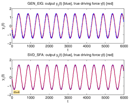
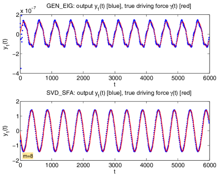
Figure 1: Each diagram shows the SFA-output $y_{1}(t)$ (blue dots) and the aligned true driving force $A(\gamma(t);y(t))$ (red line) (see Eq. (19)). The SFA-output was generated from a logistic map time series $w(t)$ (Eq. (17)) with parameters $q=1.2,\,\,\tau=1$ and the driving force of Eq. (16). The upper row shows the GEN_EIG implementation and the lower row the SVD_SFA implementation. Left: $m=4$, right: $m=8$. We see that already at embedding dimension $m=8$ the GEN_EIG results starts to deteriorate, since it has only an amplitude in the order of $10^{-7}$.

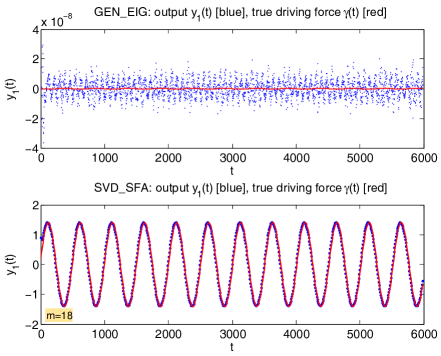
Figure 2: Same as Fig. 1, only for larger $m=12$ and $m=18$. Now the results from GEN_EIG are completely deteriorated, they are by no means slow nor do they have unit variance, while SVD_SFA still gives good results.

In the rest of this paper we will work with time series $\bm{x}(t_{i})$ instead of continuous signals $\bm{x}(t)$, but the transfer of the algorithms described above to time series is straight forward. The time derivative is simply computed as the difference between successive data points assuming a constant sampling spacing $\Delta t=1$.

3 Experiments

In the following we present examples with time series $w(t)$ derived from a logistic map to illustrate the results with different implementations of SFA. The underlying driving force is denoted by $\gamma(t)$ and may vary between $-1$ and $1$ smoothly and considerably slower (as defined by the variance of its time derivative (3)) than the time series $w(t)$. The approach follows closely the work of Wiskott Wis (03) and own previous work Kon (09), using a very simple driving force in the shape of just one sinusoidal frequency component:

$$\gamma(t)=\sin(0.0125t)\quad\in\quad[-1,1]$$ (16)

The logistic map is formulated with a parameter $q\in[0.1,3.9]$ allowing to control the presence or absence of chaotic motion (see Kon (09) for details):

$$w(t+1)=(4.0-q+0.1\gamma(t))w(t)(1-w(t))\,,$$ (17)

Taking the time series $w(t)$ directly as an input signal would not give SFA enough information to estimate the driving force, because SFA considers only data (and its derivative) from one time point at a time. Thus it is necessary to generate an embedding-vector time series as an input. Here embedding vectors at time point $t$ with delay $\tau$ and dimension $m$ are defined by

$$\bm{x}(t) := [w(t-\tau(m-1)/2),\,w(t-\tau((m-1)/2-1)),\,...,w(t+\tau(m-1)/2)]^{T}\,,$$ (18)

for scalar $w(t)$ and odd $m$. The definition can be easily extended to even $m$, which requires an extra shift of the indices by $\tau/2$ or its next lower integer to center the used data points at $t$. Centering the embedding vectors results in an optimal temporal alignment between estimated and true driving force.

In order to inspect visually the agreement between a slow SFA-signal and the driving force $\gamma(t)$ we must bring the driving force into alignment with $y(t)$ (the scale and offset of slow signals $y(t)$ extracted by SFA are arbitrarily fixed by the constraints and the sign is random). Therefore we define an $y$-aligned signal

$$A(\gamma(t);y(t))=a\gamma(t)+b$$ (19)

where the constants $a$ and $b$ are chosen in such a way that

$$E\left[(a\gamma(t)+b-y(t))^{2}\right]\stackrel{{\scriptstyle!}}{{=}}Min.$$ (20)

Table 1: Results from the implementation experiments where index $G$ denotes GEN_EIG and index $S$ denotes SVD_SFA. $m$: embedding dimension, $N_{G}$: number of eigenvalues of the generalized eigenvalue equation, $N_{S}$: number of eigenvalues of $\mbox{Cov}(\dot{\bm{z}})$, the constraints $E\left[y_{1}\right]$ and $E\left[y_{1}^{2}\right]$ acc. to Eq. (4), Eq. (5) and the slowness indicator $\eta$ WS (02); Kon (09). Low $\eta$-values indicate slow signals, high $\eta$-values fast signals. For algorithm GEN_EIG and embedding dimension $m\geq 8$ neither the unit variance constraint $E\left[y_{1}^{2}\right]_{G}=1$ nor the slowness principle for $\eta_{G}$ are fulfilled.

$m$	$N_{G}$	$N_{S}$	$E\left[y_{1}\right]_{G}$	$E\left[y_{1}\right]_{S}$	$E\left[y_{1}^{2}\right]_{G}$	$E\left[y_{1}^{2}\right]_{S}$	$\eta_{G}$	$\eta_{S}$
2	5	5	1.1e-16	-4.8e-18	1	1	11.8	11.83
4	14	9	-7.2e-16	9.0e-17	1	1	11.8	11.82
8	44	17	-1.8e-16	6.9e-17	9.5e-08	1	387.7	11.79
10	65	22	-3.2e-17	2.5e-16	1.0e-07	1	96.0	11.77
12	90	23	1.9e-16	8.8e-17	5.6e-09	1	1572.1	11.77
20	230	26	1.2e-16	-7.3e-17	6.0e-09	1	1480.3	11.76
30	495	26	1.6e-16	1.5e-17	4.7e-09	1	1661.6	11.76

The following simulations are based on 6000 data points each and were done with Matlab 7.0.1 (Release 14) as well as with Matlab 7.6.0 (R2008a) using the SFA toolkit sfa-tk Ber (03) and our extensions to it.

Fig. 1 and Fig. 2 show the results for some embedding dimensions in the case of the logistic map with $q=1.2$. The GEN_EIG results in Fig. 2 are completely corrupted by numerical errors and do not show anything ’slow’. Table 1 shows indicative numbers for the same experiment. The number of eigenvalues $N_{G}$ is always equal to the embedding dimension $M$ which is for $m\geq 8$ much larger than the true dimensionality of the expanded data. In contrast, the number $N_{S}$ of (non-zero) eigenvalues returned from SVD_SFA approaches a limiting value, in this case 26, as $m$ increases. The mean value $E\left[y_{1}\right]$ is always correct since $y_{1}$ is built from mean-free components (cf. Eq. (12)). The unit-variance constraint $E\left[y_{1}^{2}\right]_{G}=1$ is violated for $m\geq 8$ in the case of GEN_EIG. Likewise, the slowness indicator $\eta_{G}$ becomes orders of magnitude larger than $11.8$ which is the slowness of the true driving force (i.e. the signal is very fast).

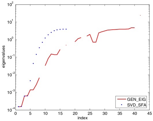
Figure 3: Eigenvalues $\lambda_{j}$ for both algorithms GEN_EIG (red line) and SVD_SFA (blue dots) for the settings of Fig. 1 and embedding dimension $m=8$, where $\bm{B}$ is singular. The red line is broken whenever a negative or complex eigenvalue occurs for GEN_EIG.

4 Discussion

We can summarize the above experiments as follows: the standard implementation GEN_EIG of SFA in sfa-tk is likely to fail if $\bm{B}$, the covariance matrix of the expanded data $\bm{v}$, becomes singular. The fact that $\bm{B}$ becomes singular indicates that the dimension of the expanded space is higher than the ’true’ dimensionality of the data. The failure can be traced back to Matlab’s routine eig(A,B) for calculating generalized eigenvalues, which is said according to Matlab’s Help to work also in the case of singular $\bm{B}$ but apparently is not.

We show in Fig. 3 the eigenvalues $\lambda_{j}$ for both algorithms GEN_EIG and SVD_SFA for one example with singular $\bm{B}$ (embedding dimension $m=8$). It is seen that in the case of GEN_EIG the line of eigenvalues is interrupted several times which is due to the fact that the corresponding eigenvalues are either negative or complex and can not be shown on a logarithmic scale. Clearly negative or complex eigenvalues should not occur for symmetric matrices $\bm{B}$ and $\bm{C^{\prime}}$. If we use SVD (command svd in Matlab) to calculate the eigenvalues of the singular, symmetric matrices $\bm{B}$ and $\bm{C}$ we find only real, nonnegative eigenvalues, as it should be.

Does a singular matrix $\bm{B}$ frequently occur?

A singular matrix $\bm{B}$ is only likely to occur if the data show a high regularity as for example in the synthesized time series of our experiments above. For data from natural sources or data with a certain amount of noise a singular $\bm{B}$ is not likely to happen, at least if the length of the time scale is not shorter than the embedding dimension. Even in our experiments with the synthesized logistic map, if we move to the chaotic region $q\leq 0.4$ then no singular $\bm{B}$ is observed, not for low and not for high embedding dimensions $m$, and the GEN_EIG algorithm of sfa-tk works as well as SVD_SFA.

Thus for natural data or for data with noise it is very unlikely to see a singular $\bm{B}$ and this is perhaps the reason why the weakness of the GEN_EIG algorithm remained so far unnoticed.

But in certain circumstances (regular data or small amount of data, as it may occur more frequently in classification applications with a limited number of patterns per class) a singular $\bm{B}$ can nevertheless happen and it is good to have with SVD_SFA a numerically stable approach.

Table 2: Rank of matrix $\bm{B}=\mbox{Cov}(\bm{v})$ as a function of embedding dimension $m$ and noise injection amplitude $\sigma_{\nu}$. $M$ is the size of the expanded signal $\bm{v}$ which equals the number of rows and columns of $\bm{B}$. For each noise amplitude lower than $\sigma_{\nu}=10^{-4}$ certain rank deficiencies occur.

	$\sigma_{\nu}$	0	$10^{-10}$	$10^{-8}$	$10^{-6}$	$10^{-4}$
$m$		$\mbox{rank}(\bm{B})$					$M$
2		5	5	5	5	5	5
4		14	14	14	14	14	14
8		24	28	31	43	44	44
10		30	39	48	64	65	65
12		32	54	69	88	90	90
20		35	141	189	227	230	230
30		35	236	406	490	495	495

Table 3: Standard deviation $E\left[y_{1}^{2}\right]$ of the slowest signal from GEN_EIG as a function of embedding dimension $m$ and noise injection amplitude $\sigma_{\nu}$. We see that even in a case where the rank-deficiency of $\bm{B}$ is only 1 out of 65 dimensions (e. g. for $m=10,\sigma_{\nu}=10^{-6}$, see Tab. 2), a constraint-violating solution might happen. In rare cases a rank-deficient $\bm{B}$ might produce a correct $y_{1}$ (e. g. for $m=8,\sigma_{\nu}=10^{-6}$), but this is more the exception than the rule.

	$\sigma_{\nu}$	0	$10^{-10}$	$10^{-8}$	$10^{-6}$	$10^{-4}$
$m$		$E\left[y_{1}^{2}\right]$
2		1	1	1	1	1
4		1	1	1	1	1
8		3e-07	4e-05	3e-05	1	1
10		1e-07	3e-07	2e-03	5e-06	1
12		8e-08	9e-05	8e-04	1	1
20		6e-08	6e-05	1e-04	5e-01	1
30		4e-09	1e-07	6e-04	1	1

Noise injection

Another way of dealing with a singular or rank-deficient $\bm{B}$ is to add to the original time series a certain amount of noise, i.e. to perform a noise injection. If we replace for example

$$w(t)\leftarrow w(t)+\nu(t)$$ (21)

where $\nu(t)$ is mean-free, normal-distributed noise with standard deviation $\sigma_{\nu}=10^{-4}$, then matrix $\bm{B}$ has full rank for all embedding dimensions $m=4,\ldots,30$, thus GEN_EIG will work as well as SVD_SFA. (Of course the data are disturbed to a certain extent.) If we try to lower $\sigma_{\nu}$ to $10^{-6},\ldots,10^{-10}$ then $\bm{B}$ becomes gradually more rank-deficient (from 1% to 50% of the dimension of $\bm{B}$) and in parallel the performance of GEN_EIG degrades in a roughly proportional way (see Tab. 2 and Tab. 3). There might be certain cases where GEN_EIG detects the correct slow signal with the correct constraints, but this can not be guaranteed.

Dependency on $\epsilon$

Is the cutoff parameter $\epsilon$ in Eq. (28) for the ’close-to-zero’-condition of eigenvalues critical for the SVD_SFA algorithm? One might suspect this to be the case since SFA in its slowest signal relies on the smallest eigenvalue. But first of all, the eigenvalues in Eq. (28) refer to $\bm{B}$ while the slowest SFA signal has a small eigenvalue in $\bm{C^{\prime}}=E\left[\dot{\bm{v}}\dot{\bm{v}}^{T}\right]$. Secondly, a small eigenvalue occuring in natural, noisy data will usually be not smaller than $10^{-3}$ while the ’close-to-zero’-condition is typically in the order of $10^{-7}\ldots 10^{-15}$ (machine accuracy) . Nevertheles we tested several other values $\epsilon=10^{-6},10^{-9},10^{-12}$ instead of the usual $10^{-7}$ and found virtually the same results. (Only $\epsilon$ as large as $10^{-5}$ resulted in a phase shift of the output signal.) Thus we conclude that the dependency on $\epsilon$ is not critical over a large range, at least not in our experiments.

5 Conclusion

We have shown that the standard SFA algorithm GEN_EIG based on generalized eigenvalues and implemented in the Matlab version of sfa-tk yields under certain circumstances wrong results (in terms of the constraints and in terms of the slowness) for the slow SFA signals due to numerical instabilities. Those circumstances can be characterized as: ”The covariance matrix $\bm{B}$ of the expanded data is rank-deficient”.

We have presented with SVD_SFA a new algorithmic implementation which follows more closely the SFA approach of Wiskott and Sejnowski WS (02) and which is numerically stable for all tested rank-deficient matrices $\bm{B}$. The Matlab-implementation is freely available for download. With a certain trick we can avoid the direct representation of the sphered expanded data and thus can implement the new SVD_SFA algorithm as efficiently as the original GEN_EIG algorithm. The new algorithm has roughly the same execution times as the old one since the time-consuming parts (expanding the data and accumulating the relevant matrices) remain the same. In our experiments the rank deficiency span a range between 1% and 90% of the number of dimensions in expanded space (see Tab. 2). The single new parameter added by SVD_SFA, namely the eigenvalue cutoff threshold $\epsilon$, was shown to be uncritical: the results obtained were insensitive to $\epsilon$-variation over a span of five decades. Thus the new algorithm does not need more parameter tuning than the old one, but it is more robust.

We have shown analytically that both implementations are equivalent as long as matrix $\bm{B}$ is regular (has full rank).

An alternative approach to reach numerical stability is to avoid rank-deficient matrices by adding a certain amount of noise to the original data (noise injection). It has been shown that the original GEN_EIG algorithm can be stabilized with the right amount of noise for all embedding dimensions $m$. Noise injection has however the drawback that certain parameters of the noise (noise amplitude, noise distribution and so on) have to be carefully tuned anew for each new SFA application.

In this work the new algorithm SVD_SFA has been applied only to driving force experiments. We plan to apply it also to SFA classification applications in the near future, where singular matrices might also occur in the case of smaller number of patterns per class.

Although we have with SVD_SFA now a robust algorithm, a general advice from the results presented here is to take always a look at rank$(\bm{B})$, the rank of the expanded data’s covariance matrix, when performing SFA. Sometimes it might be worth to think about the possible reasons for a rank deficiency (e.g. too large $m$ or too few data) and to modify the experiment conditions accordingly.

6 Appendix A

We review in this appendix some basic properties regarding covariance matrices and sphering matrices.

Given is a set of $K$ data points $\bm{v}=[v_{1},...,v_{M}]^{T}\in\Re^{M}$ with mean $\bm{v}_{0}=E\left[\bm{v}\right]$. Here $E\left[\cdot\right]$ denotes the average over all $K$ points in the set. The covariance matrix associated with $\bm{v}$ is defined as

$$\bm{B}=\mbox{Cov}(\bm{v})=E\left[(\bm{v}-\bm{v}_{0})(\bm{v}-\bm{v}_{0})^{T}\right]=E\left[\bm{v}\bm{v}^{T}\right]-\bm{v}_{0}\bm{v}_{0}^{T}$$ (22)

Usually the covariance matrix deviates from the unit matrix because it has

1. non-zero off-diagonal elements signaling dependencies between the dimensions of $\bm{v}$ and

2. varying diagonal elements showing that different dimensions of $\bm{v}$ carry different amounts of the total variance of the signal.

Case 1: $\bm{B}=\mbox{Cov}(\bm{v})$ has no zero eigenvalues.

Sphering or whitening a set of data points $\bm{v}$ means to search a linear transformation $\bm{S}$ to obtain

$$\bm{z}=\bm{S}(\bm{v}-\bm{v}_{0})\quad\mbox{such that}\quad E\left[\bm{z}\right]=0\quad\mbox{and}\quad\mbox{Cov}(\bm{z})=E\left[\bm{z}\bm{z}^{T}\right]=\bm{1}$$ (23)

If no eigenvalues are zero then the sphering transformation $\bm{S}$ exists and is given by

$$\bm{S}=\bm{D}^{-1/2}\bm{R}=\left(\begin{array}[]{ccc}1/\sqrt{\lambda_{1}}&&\\ &\cdots&\\ &&1/\sqrt{\lambda_{M}}\end{array}\right)\left(\begin{array}[]{ccc}\cdots&\bm{r}_{1}^{T}&\cdots\\[1.0pt] &\cdots&\\[1.0pt] \cdots&\bm{r}_{M}^{T}&\cdots\end{array}\right)=\left(\begin{array}[]{ccc}\cdots&\bm{r}_{1}^{T}/\sqrt{\lambda_{1}}&\cdots\\[1.0pt] &\cdots&\\[1.0pt] \cdots&\bm{r}_{M}^{T}/\sqrt{\lambda_{M}}&\cdots\end{array}\right)$$ (24)

where $\bm{r}_{k}$ is the $k$th eigenvector of $\mbox{Cov}(\bm{v})$ with eigenvalue $\lambda_{k}$ and unit length and where $\bm{R}$ is the matrix containing these eigenvectors in rows. $\bm{D}$ is the diagonal matrix of all eigenvalues. Usually, $\bm{D}$ and $\bm{R}$ are obtained by singular value decomposition (SVD). One can easily verify that

$$\bm{R}\,\mbox{Cov}(\bm{v})\,\bm{R}^{T}=\bm{D}$$ (25)

and with this

$$E\left[\bm{z}\bm{z}^{T}\right] = \bm{D}^{-1/2}\bm{R}\,E\left[(\bm{v}-\bm{v}_{0})(\bm{v}-\bm{v}_{0})^{T}\right]\,\bm{R}^{T}\bm{D}^{-1/2}$$ (26)

$$= \bm{D}^{-1/2}\underbrace{\bm{R}\,\mbox{Cov}(\bm{v})\,\bm{R}^{T}}_{=\bm{D}}\bm{D}^{-1/2}$$

$$= \bm{1}$$

An obviously equivalent way of writing this is

$$\bm{S}\,\mbox{Cov}(\bm{v})\,\bm{S}^{T}=\bm{S}\,\bm{B}\,\bm{S}^{T}=\bm{1}$$ (27)

Case 2: $\bm{B}=\mbox{Cov}(\bm{v})$ has eigenvalues $\lambda_{j}=0$.

The above sphering approach of course runs into problems if there are eigenvalues $\lambda_{j}=0$ or close to zero. The corresponding entries in $\bm{D}^{-1/2}$ would become infinity or very large and would amplify any noise or roundoff-errors multiplied with these entries. The standard trick from SVD PTVF (92) to deal with singular matrices $\bm{B}$ or $\bm{D}$ is to replace in $\bm{D}^{-1/2}$ each $1/\sqrt{\lambda}_{j}\approx 1/0$ with $0$ (!), thus effectively removing the corresponding eigenvector directions from further analysis. The condition for ’close to zero’ is defined in relation to the largest eigenvalue

$$\lambda_{j}/\lambda_{max}\leq\epsilon$$ (28)

where we usually set $\epsilon=10^{-7}$. The matrix $\bm{S}$ becomes

$$\bm{S}=\bm{D}^{-1/2}\bm{R}=\left(\begin{array}[]{ccc}1/\sqrt{\lambda_{1}}&&\\ &\cdots&\\ &&0\end{array}\right)\left(\begin{array}[]{ccc}\cdots&\bm{r}_{1}^{T}&\cdots\\[1.0pt] &\cdots&\\[1.0pt] \cdots&\bm{r}_{M}^{T}&\cdots\end{array}\right)=\left(\begin{array}[]{ccc}\cdots&\bm{r}_{1}^{T}/\sqrt{\lambda_{1}}&\cdots\\[1.0pt] &\cdots&\\[1.0pt] \cdots&0&\cdots\end{array}\right)$$ (29)

i.e. it has a $0$-row for each eigenvalue close to zero. $\bm{S}$ is not invertible, it projects into a subspace of dimension $P<M$ where $P$ is the number of non-zero eigenvalues of $\bm{B}$ (non-zero rows of $\bm{S}$). The covariance matrix $E\left[\bm{z}\bm{z}^{T}\right]=\bm{S}\,\bm{B}\,\bm{S}^{T}$ in Eq. (26) becomes now a diagonal matrix with a $1$ for each non-zero eigenvalue and a $0$ for each eigenvalue close to zero.

Our investigation above has shown that the results achieved with such a sphering approach are numerically stable in contrast to the generalized eigenvalue approach Ber (03) which has numerical problems with very small eigenvalues.

7 Appendix B: sfa-tk.V2

We briefly summarize in this appendix some information on how to obtain and use the extended package sfa-tk.V2.

The package sfa-tk.V2 with the new SVD_SFA algorithm can be downloaded from http://www.gm.fh-koeln.de/~konen/research/projects/SFA/sfa-tk.V2.zip. It is a slightly modified version of Pietro Berkes’ sfa-tk which is available from http://people.brandeis.edu/~berkes/software/sfa-tk Ber (03). Installation of sfa-tk.V2 is the same as with sfa-tk and all features of sfa-tk are maintained.

sfa-tk.V2 contains – besides the new SVD_SFA algorithm – also routines for SFA-classification, based on the ideas of Ber (05) together with Gaussian classifier routines. Two new demo scripts, namely drive1.m and class_demo2.m illustrate the usage of the new functionalities. A call of the new algorithm looks for example like

ΨΨ [y, hdl] = sfa2(x,’SVD_SFA’);

The main modifications of sfa-tk.V2 are

• lcov_pca2.m: covariance and sphering matrices are calculated with the more robust SVD method, same interface as lcov_pca.m.

• sfa_step.m: new parameter method, handed over to sfa2_step.m.

• sfa2_step.m:

  • In step ’sfa’: method=’GEN_EIG’ is the original Ber (03)-code. method=’SVD_SFA’ is the new method along the lines of [WisSej02], using lcov_pca2.m. If opts.dbg>0, then both branches are executed and their results are compared with sfa2_dbg.m.

  • In step ’expansion’: method=’TIMESERIES’ is the original Ber (03)-code where the goal is to minimize the time difference signal. The method=’CLASSIF’ is new for classification purposes, along the lines of Ber (05). Each data chunk is assumed to be a set of patterns from the same class, and the goal is to minimize the pairwise pattern difference.

• sfa2.m: new parameters method and pp_type.

• sfa2_dbg.m: perform certain debug checks and print out diagnostic information.

• drive1.m: demo script for performing the driving force demo experiments.

• class_demo2.m: demo script for performing classification experiments along the lines of Ber (05). Instead of handwritten digits we use the Vowel benchmark dataset from UCI machine learning repository (http://archive.ics.uci.edu/ml)

The full list of modifications is available in file CHANGES.htm in the download package sfa-tk.V2.zip.

8 Acknowledgment

I am grateful to Laurenz Wiskott for helpful discussions on SFA and to Pietro Berkes for providing the Matlab code for sfa-tk Ber (03). This work has been supported by the Bundesministerium für Forschung und Bildung (BMBF) under the grant SOMA (AIF FKZ 17N1009, ”Systematic Optimization of Models in IT and Automation”) and by the Cologne University of Applied Sciences under the research focus grant COSA.

References

- Ber (03) Pietro Berkes. sfa-tk: Slow Feature Analysis Toolkit for Matlab (v.1.0.1). http://people.brandeis.edu/~berkes/software/sfa-tk, 2003.
- Ber (05) Pietro Berkes. Pattern recognition with Slow Feature Analysis. Cognitive Sciences EPrint Archive (CogPrint) 4104, http://cogprints.org/4104/, 2005.
- BW (05) Pietro Berkes and Laurenz Wiskott. Slow feature analysis yields a rich repertoire of complex cells. Journal of Vision, 5(6):579 –602, 2005.
- FSW (07) Mathias Franzius, Henning Sprekeler, and Laurenz Wiskott. Slowness and sparseness lead to place, head-direction, and spatial-view cells. PLoS Comput Biol, 3(8):e166, 08 2007.
- Kon (09) Wolfgang Konen. How slow is slow? SFA detects signals that are slower than the driving force. arXiv.org e-Print archive, http://arxiv.org/abs/0911.4397v1/, 2009.
- PTVF (92) William Press, Saul Teukolsky, William Vetterling, and Brian Flannery. Numerical Recipes in C. Cambridge University Press, Cambridge, UK, 2nd edition, 1992.
- Wis (98) Laurenz Wiskott. Learning Invariance Manifolds. In Proc. of the 5th Joint Symp. on Neural Computation, May 16, San Diego, CA, volume 8, pages 196–203, San Diego, CA, 1998. Univ. of California.
- Wis (03) Laurenz Wiskott. Estimating Driving Forces of Nonstationary Time Series with Slow Feature Analysis. arXiv.org e-Print archive, http://arxiv.org/abs/cond-mat/0312317/, December 2003.
- WS (02) Laurenz Wiskott and Terrence Sejnowski. Slow Feature Analysis: Unsupervised Learning of Invariances. Neural Computation, 14(4):715–770, 2002.