Theory and Simulation of Spin Transport in Antiferromagnetic Semiconductors: Application to MnTe

Résumé

We study in this paper the parallel spin current in an antiferromagnetic semiconductor thin film where we take into account the interaction between itinerant spins and lattice spins. The spin model is an anisotropic Heisenberg model. We use here the Boltzmann’s equation with numerical data on cluster distribution obtained by Monte Carlo simulations and cluster-construction algorithms. We study the cases of degenerate and non-degenerate semiconductors. The spin resistivity in both cases is shown to depend on the temperature with a broad maximum at the transition temperature of the lattice spin system. The shape of the maximum depends on the spin anisotropy and on the magnetic field. It shows however no sharp peak in contrast to ferromagnetic materials. Our method is applied to MnTe. Comparison to experimental data is given.

I Introduction

The behavior of the spin resistivity $\rho$ as a function of temperature ($T$) has been shown and theoretically explained by many authors during the last 50 years. Among the ingredients which govern the properties of $\rho$, we can mention the scattering of the itinerant spins by the lattice magnons suggested by KasuyaKasuya , the diffusion due to impuritiesZarand , and the spin-spin correlation.DeGennes ; Fisher ; Kataoka First-principles analysis of spin-disorder resistivity of Fe and Ni has been also recently performed.Wysocki

Experiments have been performed on many magnetic materials ranging from metals to semiconductors. These results show that the behavior of the spin resistivity depends on the material: some of them show a large peak of $\rho$ at the magnetic transition temperature $T_{C}$,Matsukura others show only a change of slope of $\rho$ giving rise to a peak of the differential resistivity $d\rho/dT$.Stishov ; Shwerer Very recent experiments such as those performed on ferromagnetic SrRuO₃ thin filmsXia , Ru-doped induced ferromagnetic La_0.4Ca_0.6MnO₃Lu , antiferromagnetic $\epsilon$-(Mn_1-xFe_x)_3.25GeDu , semiconducting Pr_0.7Ca_0.3MnO₃ thin filmsZhang ,superconducting BaFe₂As₂ single crystalsWang-Chen , La_1-xSr_xMnO₃Santos and Mn_1-xCr_xTeLi compounds show different forms of anomaly of the magnetic resistivity at the magnetic phase transition temperature.

The magnetic resistivity due to the scattering of itinerant spins by localized lattice spins is proportional to the spin-spin correlation as proposed long-time ago by De Gennes and FriedelDeGennes , Fisher and LangerFisher , and recently by KataokaKataoka . They have shown that changing the range of spin-spin correlation changes the shape of $\rho$. In a recent work, Zarand et al.Zarand have showed that in magnetic diluted semiconductors the shape of the resistivity versus $T$ depends on the interaction between the itinerant spins and localized magnetic impurities which is characterized by a Anderson localization length $\zeta$. Expressing physical quantities in terms of $\zeta$ around impurities, they calculated $\rho$ and showed that its peak height depends indeed on this localization length.

In our previous workAkabli ; Akabli2 ; Akabli3 we have studied the spin current in ferromagnetic thin films. The behavior of the spin resistivity as a function of $T$ has been shown and explained as an effect of magnetic domains formed in the proximity of the phase transition point. This new concept has an advantage over the use of the spin-spin correlation since the distribution of clusters is more easily calculated using Monte Carlo simulations. Although the formation of spin clusters and their sizes are a consequence of spin-spin correlation, the direct access in numerical calculations to the structure of clusters allows us to study complicated systems such as thin films, systems with impurities, systems with high degree of instability etc. On the other hand, the correlation functions are very difficult to calculate. Moreover, as will be shown in this paper, the correlation function cannot be used to explain the behavior of the spin resistivity in antiferromagnets where very few theoretical investigations have been carried out. One of these is the work by Suezaki and MoriMori which simply predicted that the behavior of the spin resistivity in antiferromagnets is that in ferromagnets if the correlation is short-ranged. It means that correlation should be limited to ”selected nearest-neighbors”. Such an explanation is obviously not satisfactory in particular when the sign of the correlation function between antiparallel spin pairs are taken into account. In a work with a model suitable for magnetic semiconductors, Haas has shown that the resistivity $\rho$ in antiferromagnets is quite different from that of ferromagnets.Haas In particular, he found that while ferromagnets show a peak of $\rho$ at the magnetic transition of the lattice spins, antiferromagnets do not have such a peak. We will demonstrate that all these effects can be interpreted in terms of clusters used in our model.

In this paper, we introduce a simple model which takes into account the interaction between itinerant spins and localized lattice spins. This is similar to the $s-d$ modelHaas . The lattice spins interact with each other via antiferromagnetic interactions. The model will be studied here by a combination of Monte Carlo simulation and the Boltzmann’s equation. As will be discussed below, such a model corresponds to antiferromagnetic semiconductors such as MnTe. An application is made for this compound in the present work.

The paper is organized as follows. In section II, we show and discuss our general model and its application to the antiferromagnetic case using the Boltzmann’s equation formulated in terms of clusters. We also describe here our Monte Carlo simulations to obtain the distributions of sizes and number of clusters as functions of $T$ which will be used to solve the Boltzmann’s equation. Results on the effects of Ising-like anisotropy and magnetic field as well as an application to the case of MnTe is shown in section III. Concluding remarks are given in section IV.

II Theory

Let us recall briefly principal theoretical models for magnetic resistivity $\rho$. In magnetic systems, de Gennes and FriedelDeGennes have suggested that the magnetic resistivity is proportional to the spin-spin correlation. As a consequence, in ferromagnetically ordered systems, $\rho$ shows a divergence at the transition temperature $T_{C}$, similar to the susceptibility. However, in order to explain the finite cusp of $\rho$ experimentally observed in some experiments, Fisher and LangerFisher suggested to take into account only short-range correlations in the de Gennes-Friedel’s theory. KataokaKataoka has followed the same line in proposing a model where he included, in addition to a parameter describing the correlation range, some other parameters describing effects of the magnetic instability, the density of itinerant spins and the applied magnetic field.

For antiferromagnetic systems, Suezaki and MoriMori proposed a model to explain the anomalous behavior of the resistivity around the Néel temperature. They used the Kubo’s formula for an $s-d$ Hamiltonian with some approximations to connect the resistivity to the correlation function. However, it is not so easy to resolve the problem. Therefore, the form of the correlation function was just given in the molecular field approximation. They argued that just below the Néel temperature $T_{N}$ a long-range correlation appears giving rise to an additional magnetic potential which causes a gap. This gap affects the electron density which alters the spin resistivity but does not in their approximation interfere in the scattering mechanism. They concluded that, under some considerations, the resistivity should have a peak close to the Néel point. This behavior is observed in $Cr$, $\alpha-Mn$ and some rare earth metals. Note however that in the approximations used by HaasHaas , there is no peak predicted. So the question of the existence of a peak in antiferromagnets remains open.

Following Haas, we use for semiconductors the following interaction

$$V=\sum_{n}J(\vec{r}-\vec{R}_{n})\mathbf{s}\cdot\mathbf{S}_{n}$$ (1)

where $J(\vec{r}-\vec{R}_{n})$ is the exchange interaction between an itinerant spin $\mathbf{s}$ at $\vec{r}$ and the lattice spin $\mathbf{S}_{n}$ at the lattice site $\vec{R}_{n}$. In practice, the sum on lattice spins $\mathbf{S}_{n}$ should be limited at some cut-off distance as will be discussed later. Haas supposed that $V$ is weak enough to be considered as a perturbation to the lattice Hamiltonian given by Eq. (15) below. This is what we also suppose in the present paper. He applied his model to ferromagnetic doped CdCr₂Se₄Lehmann ; Shapira ; Snyder and antiferromagnetic semiconductors MnTe. Note however that the model by Haas as well as other existing models cannot treat the case where itinerant spins, due to the interaction between themselves, induce itinerant magnetic ordering such as in (Ga,Mn)As shown by Matsukura et al.Matsukura Note also that both the up-spin and down-spin currents are present in the theory but the authors considered only the effect of the up-spin current since the interaction ”itinerant spin”-”lattice spin” is ferromagnetic so that the down-spin current is very small. This theory was built in the framework of the relaxation-time approximation of the Boltzmann’s equation under an electric field. As De Gennes and Friedel, Haas used here the spin-spin correlation to describe the scattering of itinerant spins by the disorder of the lattice spins. As a result, the model of Haas shows a peak in the ferromagnetic case but no peak in the antiferromagnetic semiconductors. Experimentally, the absence of a peak has been observed in antiferromagnetic LaFeAsO by McGuire et al.McGuire and in CeRhIn₅ by Christianson et al.Christianson

II.1 Boltzmann’s equation

In the case of Ising spins in a ferromagnet that we studied beforeAkabli3 , we have made a theory based on the cluster structure of the lattice spins. The cluster distribution was incorporated in the Boltzmann’s equation. The number of clusters $\eta$ and their sizes $\xi$ have been numerically determined using the Hoshen-Kopelmann’s algorithm (section II.2).Hoshen We work in diffusive regime with approximation of parabolic band and in an $s-d$ model. We consider in this paper that in our range of temperature the Hall resistivity is constant (constant density). To work with the Born approximation we consider a weak potential of interaction between clusters of spin and conduction electrons. We suppose that the life’s time of clusters is larger than the relaxation time. As in our previous paperAkabli3 we use in this paper the expression of relaxation time obtained from the Boltzmann’s equation in the following manner. We first write the Boltzmann’s equation for $f$, the distribution function of itinerant electrons, in a uniform electric field E

$$(\dfrac{\hbar\textbf{k}.e\textbf{E}}{m})(\dfrac{\partial f^{0}}{\partial\varepsilon})=(\dfrac{\partial f}{\partial t})_{coll},$$ (2)

where $f^{0}$ is the equilibrium Fermi-Dirac function, k the wave vector, $e$ and $m$ the electronic charge and mass, $\epsilon$ the electron energy. We next use the following relaxation-time approximation

$$(\dfrac{\partial f_{k}}{\partial t})_{coll}=-(\dfrac{f_{k}^{1}}{\tau_{k}}),\qquad f_{k}^{1}=f_{k}-f_{k}^{0},$$ (3)

where $\tau_{k}$ is the relaxation time. Supposing elastic collisions, i. e. $k=k^{\prime}$, and using the detailed balance we have

$$(\dfrac{\partial f_{k}}{\partial t})_{coll}=\dfrac{\Omega}{(2\pi)^{3}}\int[w_{k^{\prime},k}(f^{1}_{k^{\prime}}-f^{1}_{k})]d\mathbf{k^{\prime}},$$ (4)

where $\Omega$ is the system volume, $w_{k^{\prime},k}$ the transition probability between k and $\textbf{k}^{\prime}$. We find with Eq. (3) and Eq. (4) the following well-known expression

$$(\dfrac{1}{\tau_{k}}) = \dfrac{\Omega}{(2\pi)^{3}}\int[w_{k^{\prime},k}(1-\cos\theta)]$$ (5)

$$\times\sin\theta k^{\prime 2}dk^{\prime}d\theta d\phi,$$

where $\theta$ and $\phi$ are the angles formed by $\textbf{k}^{\prime}$ with k, i. e. spherical coordinates with $z$ axis parallel to $\mathbf{k}$.

We use now in Eq. (5) the ”Fermi golden rule” for $\omega_{k,k^{\prime}}$ and we obtain

$$\dfrac{1}{\tau_{k}}=\dfrac{\Omega}{(2\pi)^{3}}\int[\omega_{k,k^{\prime}}(1-cos(\theta))]sin(\theta)k^{\prime 2}dk^{\prime}d\theta d\phi$$ (6a)

$$\omega_{k,k^{\prime}}=\dfrac{(2\pi)m}{\hbar^{3}k}|<k^{\prime}|J(r)|k>|^{2}\delta(k^{\prime}-k)$$ (6b)

where $J(r)$ is the exchange integral between an itinerant spin and a lattice spin which is given in the scattering potential, Eq. (1). One has

$$J(r)\equiv J(|\vec{r}^{\prime}-\vec{R}_{n}|)$$ (7)

Note that for simplicity we have supposed here that the interaction potential $J(r)$ depends only on the relative distance $r^{\prime}=|\vec{r}-\vec{R}_{n}|$, not on the direction of $\vec{r}-\vec{R}_{n}$. We suppose in the following a potential which exponentially decays with distance

$$J(r)\equiv V_{0}e^{-r/\xi}$$ (8)

where $V_{0}$ expresses the magnitude of the interaction and $\xi$ the averaged cluster size. After some algebra, we arrive at the following relaxation time

$$\dfrac{1}{\tau_{k_{f}}}=\dfrac{32V_{0}^{2}m\pi}{(2k\hbar)^{3}}\eta\xi^{2}[1-\dfrac{1}{1+(2\xi k_{f})^{2}}-\dfrac{(2\xi k_{f})^{2}}{[1+(2\xi k_{f})^{2}]^{2}}]$$ (9)

where $k_{f}$ is the Fermi wave vector. As noted by HaasHaas , the mobility is inversely proportional to the susceptibility $\chi$. So, in examining our expression and in using the following expression $\chi=\sum\xi^{2}\eta(\xi)$,Binder where $\eta(\xi)$ is the number of clusters of size $\xi$, one sees that the first term of the relaxation time is proportional to the susceptibility. The other two terms are the corrections.

The mobility in the $x$ direction is defined by

$$\mu_{x}=\dfrac{e\hbar^{2}}{3m^{2}}\dfrac{\sum_{k}k^{2}(\partial f^{0}_{k}/\partial\epsilon)\tau_{k}}{\sum_{k}f^{0}_{k}}$$ (10)

We resolve the mobility $\mu_{x}$ explicitly in the following two cases

• Degenerate semiconductors

  $$\sum_{k}f^{0}_{k}=2\pi(\dfrac{2m}{\hbar^{2}})^{3/2}[\dfrac{2}{3}\epsilon_{f}^{3/2}]$$ (11a)

  $$\sum_{k}k^{2}(\partial f^{0}_{k}/\partial\epsilon)\tau_{k}=2\pi(\dfrac{2m}{\hbar^{2}})^{3/2}\dfrac{\epsilon_{f}^{1/2}}{D}(\dfrac{2m\epsilon_{f}}{\hbar^{2}})^{5/2}[\dfrac{1+8m\xi^{2}\epsilon_{f}/\hbar^{2}}{8m\xi^{2}\epsilon_{f}/\hbar^{2}}]^{2}$$ (11b)

  where $D=\dfrac{\eta 4V_{0}^{2}m\pi\xi^{2}}{\hbar^{3}}$. We arrive at the following mobility

  $$\mu_{x}=\dfrac{e\hbar^{2}}{2m^{2}}\dfrac{\epsilon_{f}^{-1}}{D}(\dfrac{2m\epsilon_{f}}{\hbar^{2}})^{5/2}[\dfrac{1+8m\xi^{2}\epsilon_{f}/\hbar^{2}}{8m\xi^{2}\epsilon_{f}/\hbar^{2}}]^{2}$$ (12a)

  $$\sigma=ne\mu=\dfrac{ne^{2}}{mDk_{f}}[\dfrac{1+4\xi^{2}k^{2}_{f}}{4\xi^{2}}]^{2}$$ (12b)

  The resistivity is then

  $$\rho=\dfrac{\eta 4V_{0}^{2}m^{2}\pi k_{f}\xi^{2}}{ne^{2}\hbar^{3}}[\dfrac{4\xi^{2}}{1+4\xi^{2}k^{2}_{f}}]^{2}$$ (13a)

  We can check that the right-hand side has the dimension of a resistivity: $\dfrac{[kg][m]^{3}}{[C]^{2}[s]}=[\Omega][m]$.

• Non-degenerate semiconductors

  One has in this case $f_{k}^{0}=exp(-\beta\epsilon_{k})$
  

  $$\sum_{k}f^{0}_{k}=2\pi(\dfrac{2m}{\hbar^{2}})^{3/2}\beta^{-3/2}\sqrt{\pi}/2$$ (14a)

  $$\sum_{k}k^{2}(\partial f^{0}_{k}/\partial\epsilon)\tau_{k}=2\pi(\dfrac{2m}{\hbar^{2}})^{3/2}\dfrac{1}{2D(4\xi^{2})^{2}\beta}(\dfrac{2m}{\hbar^{2}})^{1/2}[1+\dfrac{2\times 16m\xi^{2}}{\hbar^{2}\beta}+\dfrac{6(8m\xi^{2})^{2}}{\hbar^{4}\beta^{2}}]$$ (14b)

  $$\sigma=ne\mu=\dfrac{ne^{2}\hbar^{2}}{m^{2}D(4\xi^{2})^{2}\sqrt{\pi}}(\dfrac{2m\beta}{\hbar^{2}})^{1/2}[1+\dfrac{2\times 16m\xi^{2}}{\hbar^{2}\beta}+\dfrac{6(8m\xi^{2})^{2}}{\hbar^{4}\beta^{2}}]$$ (14c)

  $$\rho=\dfrac{1}{\sigma}$$ (14d)

  where $D=\dfrac{\eta 4V_{0}^{2}m\pi\xi^{2}}{\hbar^{3}}$

Note that the formulation of our theory in terms of cluster number $\eta$ and cluster size $\xi$ is numerically very convenient. These quantities are easily calculated by Monte Carlo simulation for the Ising model. The method can be generalized to the case of Heisenberg spins where the calculation is more complicated as seen below. In section III.1 we will examine values of parameter $V_{0}$ where the Born’s approximation is valid.

II.2 Algorithm of Hoshen-Kopelmann and Wolff’s procedure

We use the Heisenberg spin model with an Ising-like anisotropy for an antiferromagnetic film of body-centered cubic (BCC) lattice of $N_{x}\times N_{y}\times N_{z}$ cells where there are two atoms per cell. The film has two symmetrical (001) surfaces, i.e. surfaces perpendicular to the $z$ direction. We use the periodic boundary conditions in the $xy$ plane and the mirror reflections in the $z$ direction. The lattice Hamiltonian is written as follows

$$\mathcal{H}=J\sum_{\left<i,j\right>}\mathbf{S}_{i}\cdot\mathbf{S}_{j}+A\sum_{\left<i,j\right>}S^{z}_{i}S^{z}_{j}$$ (15)

where $\mathbf{S}_{i}$ is the Heisenberg spin at the site $i$, $\sum_{\left<i,j\right>}$ is performed over all nearest-neighbor (NN) spin pairs. We assume here that all interactions including those at the two surfaces are identical for simplicity: $J$ is positive (antiferromagnetic), and $A$ an Ising-like anisotropy which is a positive constant. When $A$ is zero, one has the isotropic Heisenberg model and when $A\rightarrow\infty$, one has the Ising model. The classical Heisenberg spin model is continuous, so it allows the domain walls to be less abrupt and therefore softens the behavior of the magnetic resistance. Note that for clarity of illustration, in this section (II.B) we suppose only NN interaction $J$. In the application to MnTe shown in section III.C, the exchange integral is distance-dependent and we shall take into account up to the third NN interaction.

Hereafter, the temperature is expressed in unit of $J/k_{B}$, $k_{B}$ being the Boltzmann’s constant. $A$ is given in unit of $J$. The resistivity $\rho$ is shown in atomic units.

For the whole paper, we use $N_{x}=N_{y}=20$, and $N_{z}=8$. The finite-size effect as well as surface effects are out of the scope of the present paper. Using the Hamiltonian (15), we equilibrate the lattice at a temperature $T$ by the standard Monte Carlo simulation. In order to analyze the spin resistivity, we should know the energy landscape seen by an itinerant spin. The energy map of an itinerant electron in the lattice is obtained as follows: at each position its energy is calculated using Eq. (8) within a cutoff at a distance $D_{1}=2$ in unit of the lattice constant $a$. The energy value is coded by a color as shown in Fig. 1 for the case $A=0.01$. As seen, at very low $T$ ($T=0.01$) the energy map is periodic just as the lattice, i. e. no disorder. At $T=1$, well below the Néel temperature $T_{N}\simeq 2.3$, we observe an energy map which indicates the existence of many large defect clusters of high energy in the lattice. For $T\approx T_{N}$ the lattice is completely disordered. The same is true for $T=2.5$ above $T_{N}$.

We shall now calculate the number of clusters and their sizes as a function of $T$ in order to analyze the temperature-dependent behavior of the spin current.

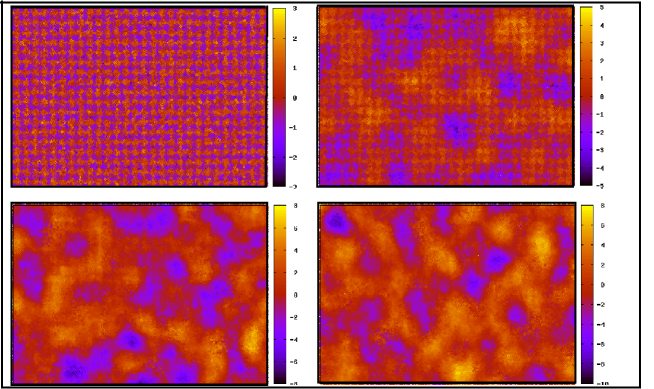
Figure 1: Energy map of an itinerant spin in the $xy$ plane with $D_{1}=2$ in unit of the lattice constant $a$ and $A=0.01$, for $T=0.01$, $T=1.0$, $T=2.0$ and $T=2.5$ (from left to right, top to bottom, respectively). The values of energy corresponding to different colors are given on the right.

The scattering by clusters in the Ising case in our previous modelAkabli3 is now replaced in the Heisenberg spin model studied here, by a scattering due to large domain walls. Counting the number of clusters in the Heisenberg case requires some particular attention as seen in the following:

• we equilibrate the system at $T$

• we generate first bonds according to the algorithm by Wolff:Wolff2 ; Wolff it consists in replacing the two spins where the link is verified the Wolff’s probability, by their larger value (Fig 2)

• we next discretize $S_{z}$, the $z$ component of each spin, into values between $-1$ and $1$ with a step $0.1$

• only then we can use the algorithm of Hoshen-Kopelmann to form a cluster with the neighboring spins of the same $S_{z}$. This is how our clusters in the Heisenberg case are obtained.

Note that we can define a cluster distribution by each value of $S_{z}$. We can therefore distinguish the amplitude of scattering: as seen below scattering is stronger for cluster with larger $S_{z}$.

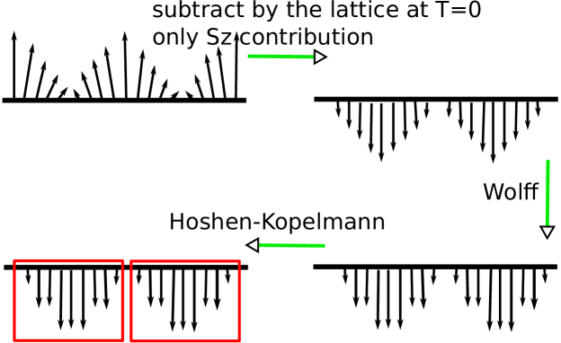
Figure 2: The successive steps in the application of the algorithm by Wolff to the case of Heisenberg spin. See text for explanation.

We have used the above procedure to count the number of clusters in our simulation of an antiferromagnetic thin film. We show in Fig. 3 the number of cluster $\eta$ versus $T$ for several values of $S_{z}$.

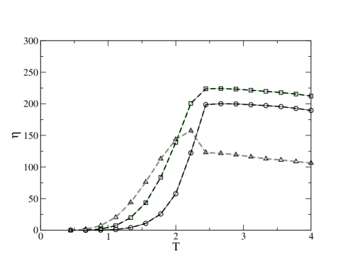
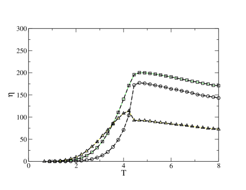
Figure 3: Number of clusters versus temperature for anisotropy $A=0.01$ (upper) and $A=1$ (lower). The values of $S_{z}$ are 1, 0.8 and 0.6 denoted by circles, squares and triangles, respectively. Lines are guides to the eye.

We have in addition determined the average size of these clusters as a function of $T$. The results are shown in Fig. 4. One observes that the size and the number of clusters of any value of $S_{z}$ change the behavior showing a maximum at the transition temperature.

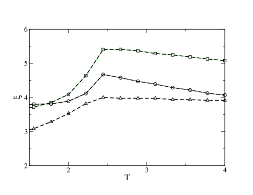
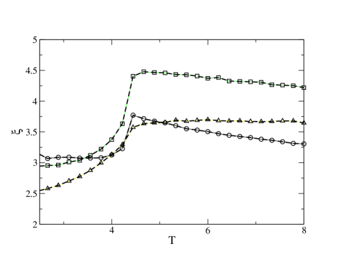
Figure 4: Average size of clusters versus temperature for anisotropy $A=0.01$ (upper) and $A=1$ (lower). The values of $S_{z}$ are 1, 0.8 and 0.6 denoted by circles, squares and triangles, respectively. Lines are guides to the eye.

The resistivity, as mentioned above, depends indeed on the amplitude of $S_{z}$ as seen in the expression

$$\rho=\dfrac{m}{ne^{2}}\dfrac{1}{\tau}=\dfrac{m}{ne^{2}}\sum^{S_{z}}_{i=-S_{z}}\dfrac{1}{\tau_{i}}$$ (16)

III Results

III.1 Effect of Ising-like Anisotropy

At this stage, it is worth to return to examine some fundamental effects of $V_{0}$ and $A$. It is necessary to know acceptable values of $V_{0}$ imposed by the Born’s approximation. To do this we must calculate the resistivity with the second order Born’s approximation.

$$\sigma_{k}^{B}(\theta,\phi)=|\dfrac{F(\theta,\phi)}{4\pi}|^{2}$$ (17a)

$$F(\theta,\phi)=\dfrac{2m\Omega}{\hbar^{2}}[\int d^{3}re^{-i{\bf K}.{\bf r}}J(r)-\dfrac{1}{4\pi}\int d^{3}re^{-i{\bf K}.{\bf r}}\dfrac{J(r)}{r}\int d^{3}r^{\prime}e^{-i{\bf K}.{\bf r^{\prime}}}J(r^{\prime})]$$ (17b)

$$K=|{\bf k}-{\bf k}^{\prime}|=k[2(1-\cos\theta)]^{1/2}\ \mbox{and}\ J(r)=V_{0}e^{-r/\xi}$$

we find, with $D=\dfrac{\eta 32\pi\Omega m}{\hbar^{3}}$,

$$\dfrac{1}{\tau_{k}}=DV_{0}^{2}k[\dfrac{2\xi^{6}}{[1+(2\xi k)^{2}]^{2}}-\dfrac{V_{0}}{3[1+(2\xi k)^{2}]^{2}}(1+\dfrac{4}{[1+(2\xi k)^{2}]^{2}})+\dfrac{V_{0}^{2}\xi^{6}}{12(2k^{2})^{2}}]$$ (18)

The first term is due to the first order of Born’s approximation and the second and third terms to corrections from the second order. We plot $\rho(Born2)/\rho(Born1)$ versus $T$ in Fig. 5 for different values of $V_{0}$, $\rho(Born1)$ and $\rho(Born2)$ being respectively the resistivities calculated at the first and second order. We note that the larger this ratio is, the more important the corrections due to the second-order become. From Fig. 5, several remarks are in order:

• The first order of Born’s approximation is valid for small values of $V_{0}$ as seen in the case $V_{0}=0.01$ corresponding to a few meV. In this case the resistivity does not depend on $T$. This is understandable because with such a weak coupling to the lattice, itinerant spins do not feel the effect of the lattice spin disordering.

• In the case of strong $V_{0}$ such as $V_{0}=0.05$, the second-order approximation should be used. Interesting enough, the resistivity is strongly affected by $T$ with a peak corresponding to the phase transition temperature of the lattice.

Figure 5: Ratio Residue=$\rho(Born2)/\rho(Born1)$ versus $T$ for $V_{0}$=0.05 (squares, upper curve) and 0.01 (circles, lower curve). See text for comments.

We examine now the effect $A$. Figure 6 shows the variation of the sublattice magnetization and of $T_{N}$ with anisotropy $A$. We have obtained respectively for $A=0.01$, $A=1$, $A=1.5$ and pure Ising case the following critical temperatures $T_{N}\simeq 2.3$, $4.6$, $5.6$ and $6.0$. Note that the pure Ising case has been simulated with the pure Ising Hamiltonian, not with Eq. (15) (we cannot use $A=\infty$). We can easily understand that not only the spin resistivity will follow this variation of $T_{N}$ but also the change of $A$ will fundamentally alter the resistivity behavior as will be seen below.

Figure 6: Sublattice magnetization versus $T$ for several values of anisotropy $A$. From left to right $A=0.01$, $A=1$, $A=1.5$ and pure Ising spin.

The results shown in Fig. 7 indicate clearly the appearance of a peak at the transition which diminishes with increasing anisotropy. If we look at Fig. 4 which shows the average size of clusters as a function of $T$, we observe that the size of clusters of large $S_{z}$ diminishes with increasing $A$.

We show in Fig. 8 the pure Heisenberg and Ising models. For the pure Ising model, there is just a shoulder around $T_{N}$ with a different behavior in the paramagnetic phase: increase or decrease with increasing $T$ for degenerate or non degenerate cases. It is worth to mention that MC simulations for the pure Ising model on the simple cubic and BCC antiferromagnets where interactions between itinerant spins are taken into account in addition to Eq. (1), show no peak at allMagnin ; Magnin2 . These results are in agreement with the tendency observed here for increasing $A$.

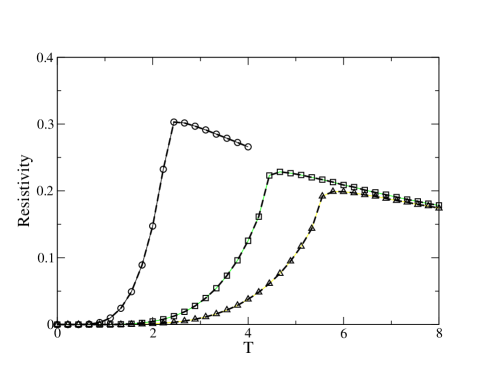
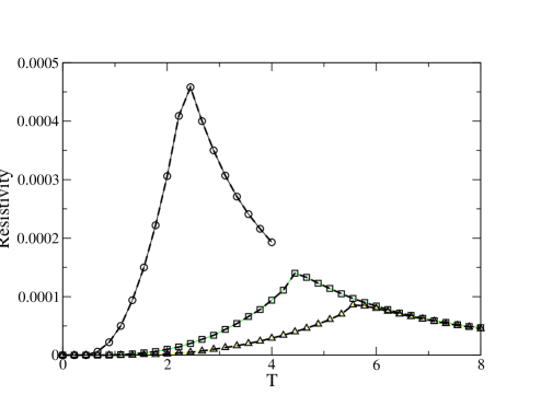
Figure 7: Spin resistivity versus $T$ for several anisotropy values $A$ in antiferromagnetic BCC system: $A=0.01$ (circles), 1 (squares), 1.5 (triangles). Upper (lower) curves: degenerate (non degenerate) system.

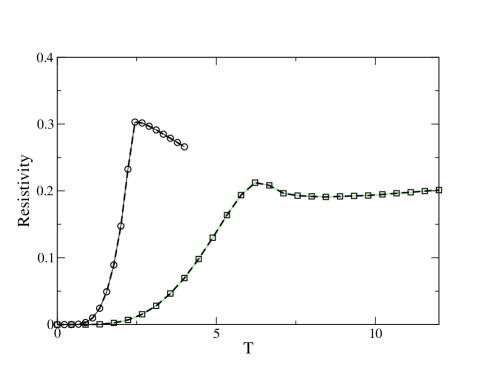
Figure 8: Spin resistivity for pure Heisenberg (circles) and Ising (squares) models in antiferroamgnetic BCC system. Upper (lower) curves: degenerate (non degenerate) system.

III.2 Effect of Magnetic Field

We apply now a magnetic field perpendicularly to the electric field. To see the effect of the magnetic field it suffices to replace the distribution function by

$$f^{1}_{k}=\dfrac{e\hbar\tau_{k}}{m}(-\frac{\partial f^{0}}{\partial\epsilon})\textbf{k}.\dfrac{(\textbf{E}-\dfrac{e\tau_{k}}{mc}\textbf{H}\wedge\textbf{E})}{1+(\dfrac{e\tau_{k}H}{mc})^{2}}$$ (19)

From this, we obtain the following equations for the contributions of up and down spins

$$\rho_{\downarrow}=\sum^{+1}_{S_{z}=-1}(S_{z}+1)^{2}\dfrac{\eta 4V_{0}^{2}m^{2}\pi k_{f}\xi^{2}}{ne^{2}\hbar^{3}}[\dfrac{4\xi^{2}}{1+4\xi^{2}k^{2}_{f}}]^{2}$$ (20)

$$\rho_{\uparrow}=\sum^{+1}_{S_{z}=-1}(S_{z}-1)^{2}\dfrac{\eta 4V_{0}^{2}m^{2}\pi k_{f}\xi^{2}}{ne^{2}\hbar^{3}}[\dfrac{4\xi^{2}}{1+4\xi^{2}k^{2}_{f}}]^{2}$$ (21)

where $S_{z}$ is the domain-wall spin (scattering centers) and $V_{0}$ is the coefficient of the exchange integral between an itinerant spin and a lattice spin [see Eq. (8)].

Figures 9 and 10 show the resistivity for several magnetic fields. We observe a split in the resistivity for up and down spins which is larger for stronger field. Also, we see that the minority spins shows a smaller resistivity due to their smaller number. The reason is similar to the effect of $A$ mentioned above and can be understood by examining Fig. 11 where we show the evolution of the number and the average size of clusters with the temperature in a magnetic field. By comparing with the zero-field results shown in Figs. 3 and 4, we can see that while the number of clusters does not change with the applied field, the size of clusters is significantly bigger. It is easy to understand this situation: when we apply a magnetic field, the spins want to align themselves to the field so the up-spin domains become larger, critical fluctuations are at least partially suppressed, the transition is softened.

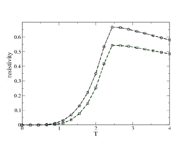
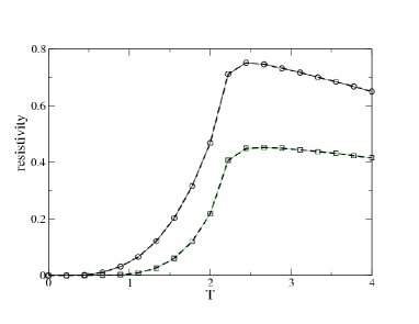
Figure 9: Resistivities of up (circles) and down (squares) spins versus $T$ for two magnetic field’s strengths in the degenerate case. Top (bottom): $B=0.6(1.5)$.

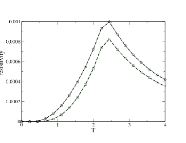
Figure 10: Resistivities of up (circles) and down (squares) spins versus $T$ for two magnetic field’s strengths in the non degenerate case. Top (bottom): $B=0.6(1.5)$.

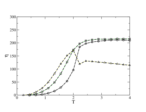
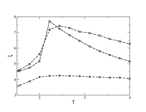
Figure 11: Upper: Number of clusters, Lower: Average size of clusters, versus $T$ for several values of $S_{z}$ and for magnetic field $B=1.5$. Circles: $S_{z}=1$, squares: $S_{z}=0.8$, triangles: $S_{z}=0.6$. Lines are guides to the eye.

III.3 Application to MnTe

We have chosen a presentation of the general model which can be applied to degenerate and non-degenerate semiconductors and semi metals. The application to hexagonal MnTe is made below with the formulae of both degenerate and non-degenerate cases, for comparison. Hexagonal MnTe has a big gap (1.27 eV), but it is an indirect gap. So, thermal excitations of electrons to the conduction band may not need to cross the gap channel. This may justify the use of the degenerate formulae. In the degenerate case, $k_{f}$ depends only on the carrier concentration $n$ via the known formula: $k_{f}=(3\pi^{2}n)^{1/3}$ . We use for MnTe $n=2\times 10^{22}$cm^-3 mentioned below. For the non-degenerate case, $k_{f}$ is not necessary. Note that in the case of pure intrinsic semiconductors, $k_{f}$ is in the gap and its position is given by the law of mass action using parabolic band approximation. In doped cases, band tails created by doped impurities can cover more or less the gap. But this system, which is disordered by doping, is not a purpose of our present study.

In semiconductors valence electrons can go from the valence band to the conduction band more and more as the temperature increases. Therefore, the carrier concentration is a function of $T$. Our model has a number of itinerant spins which is independent of $T$ in each simulation. However in each simulation, we can take another concentration (see Ref. 19): the results show that the resistivity is not strongly modified, one still has the same feature, except that the stronger the concentration is the smaller the peak at $T_{C}$ becomes if and only if interaction between itinerant spins is taken into account. Therefore, we believe that generic effects independent of carrier concentration will remain. Of course, the correct way is to use a formula to generate the carrier concentration as a function of $T$ and to make the simulation with the temperature-dependent concentration taking account additional scattering due to interaction between itinerant spins. Unfortunately, to obtain that formula we have to use several approximations which involve more parameters. We will try this in a future work.

In the case of Cd_1-xMn_xTe, the question of the crystal structure, depending on the doping concentration $x$ remains open. Cd_1-xMn_xTe can have one of the following structures, the so-called NiAs structure or the zinc-blend one, or a mixed phase.Komatsubara ; Szwacki ; Wei ; Adachi

The pure MnTe crystallizes in either the zinc-blend structureHennion or the hexagonal NiAs oneHennion2 (see Fig. 12). MnTe is a well-studied $p$-type semiconductor with numerous applications due to its high Néel temperature. We are interested here in the case of hexagonal structure. For this case, the Néel temperature is $T_{N}=310$ KHennion2 .

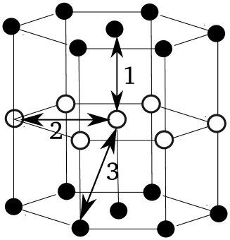
Figure 12: Structure of the type NiAs is shown with Mn atoms only. This is a stacked hexagonal lattice. Up spins are shown by black circles, down spins by white ones. Nearest-neighbor (NN) bond is marked by 1, next NN bond by 2, and third NN bond by 3.

The cell parameters are $a=4.158\AA$ and $c=6.71\AA$ and we have an indirect band gap of $E_{g}=1.27$eV.

Magnetic properties are determined mainly by an antiferromagnetic exchange integral between nearest-neighbors (NN) Mn along the $c$ axis, namely $J_{1}/k_{B}=-21.5\pm 0.3$ K, and a ferromagnetic exchange $J_{2}/k_{B}\approx 0.67\pm 0.05$ between in-plane (next NN) Mn. Third NN interaction has been also measured with $J_{3}/k_{B}\simeq-2.87\pm 0.04$ K. Note that the spins are lying in the $xy$ planes perpendicular to the $c$ direction with an in-plane easy-axis anisotropyHennion2 . The magnetic structure is therefore composed of ferromagnetic $xy$ hexagonal planes antiferromagnetically stacked in the $c$ direction. The NN distance in the $c$ direction is therefore $c/2\simeq 3.36$ shorter than the in-plane NN distance $a$.

Figure 13: Number of clusters (upper) and cluster size (lower) versus $T$ for MnTe structure obtained from Monte Carlo simulations for several values of $S_{z}$: 1 (circles), 0.8 (squares), 0.6 (triangles). Lines are guides to the eye.

We have calculated the cluster distribution for the hexagonal MnTe using the exchange integrals taken from Ref. Hennion2 and the other crystal parameters taken from the literatureInoue ; Okada ; Chandra . The result is shown in Fig. 13. The spin resistivity in MnTe obtained with our theoretical model is presented in Fig. 14 for a density of itinerant spins corresponding to $n=2\times 10^{22}$ cm^-3, together with ”normalized” experimental data. The normalization has been made by noting that the experimental resistivity $R$ in Ref. 41 is the total one with contributions from impurities and phonons. However, the phonon contribution is important only at high $T$, so we can neglect it for $T<310$K. While for the contribution $R_{0}$ from fixed impurities, there are reasons to consider it as temperature-independent at low $T$. From these rather rude considerations, we extract $R_{0}$ from $R$ and compare our theoretical with $R-R_{0}$. This is what we called ”normalized resistivity” in Fig. 14.

Figure 14: Normalized spin resistivity versus $T$ in MnTe : theoretical non-degenerate case (circles), theoretical degenerate case (squares) and experimental results (stars) from Chandra et alChandra . Experimental data lie on the degenerate line for $T\geq 140$ K. See text for comments.

Several remarks are in order:

i) the peak temperature of our theoretical model is found at 310 K corresponding the the experimental Néel temperature although for our fit we have used only the above-mentioned values of exchange integrals

ii) our result is in agreement with experimental data obtained by Chandra et al.Chandra for temperatures between 140 K and 280 K above which Chandra et al. did not unfortunately measured

iii) at temperatures lower than 140 K, the experimental curve increases with decreasing $T$. Note that many experimental data on various materials show this ’universal’ feature: we can mention the data by Li et al.Li , Du et al.Du , Zhang et al.Zhang , McGuire et al.McGuire among others. Our theoretical model based on the scattering by defect clusters cannot account for this behavior because there are no defects at very low $T$. Direct Monte Carlo simulation shows however that the freezing indeed occurs at low $T$ both in ferromagnetsMagnin ; Akabli3 and antiferromagnetsMagnin2 giving rise to an increase of the spin resistivity with decreasing $T$. There are several explanations for this experimental behavior among which we can mention the fact that in semiconductors the carrier concentration increases as $T$ increases, giving rise to an increase of the spin current, namely a decrease of the resistivity, with increasing $T$ in the low-$T$ region. Another origin of the increase of $\rho$ as $T\rightarrow 0$ is the possibility that the itinerant electrons may be frozen (crystallized) due to their interactions with localized spins and between themselves, giving rise to low mobility. On the hypothesis of frozen electrons, there is a reference on the charge-ordering at low $T$ in Pr_0.5Ca_0.5MnO₃Zhang due to some strain interaction. A magnetic field can make this ordering melted giving rise to a depressed resistivity. Our present model does not correspond to this compound but we believe that the concept is similar. For the system Pr_0.5Ca_0.5MnO₃, which shows a commensurate charge order, the ”melting” fields at low temperatures are high, on the order of 25 TeslaZhang .

iv) the existence of the peak at $T_{N}=310$ K of the theoretical spin resistivity shown in Fig. 14 is in agreement with experimental data recently published by Li et al.Li (see the inset of their Fig. 5). Unfortunately, we could not renormalize the resistivity values of Li et al.Li to put in the same figure with our result for a quantitative comparison. Other data on various materialsDu ; McGuire ; Zhang also show a large peak at the magnetic transition temperature.

To close this section, let us note that it is also possible, with some precaution, to apply our model on other families of antiferromagnetic semiconductors like CeRhIn₅ and LaFeAsO. An example of supplementary difficulties but exciting subject encountered in the latter compound is that there are two transitions in a small temperature region: a magnetic transition at $145$ K and a tetragonal-orthorhombic crystallographic phase transition at $160$ K.McGuire ; Christianson An application to ferromagnetic semiconductors of the n-type CdCr₂Se₄Lehmann2 is under way.

IV Conclusion

We have shown in this paper the behavior of the magnetic resistivity $\rho$ as a function of temperature in antiferromagnetic semiconductors. The main interaction which governs the resistivity behavior is the interaction between itinerant spins and the lattice spins. Our analysis, based on the Boltzmann’s equation which uses the temperature-dependent cluster distribution obtained by MC simulation. Our result is in agreement with the theory by HaasHaas : we observe a broad maximum of $\rho$ in the temperature region of the magnetic transition without a sharp peak observed in ferromagnetic materials. We have studied the two cases, degenerate and non-degenerate semiconductors. The non-degenerate case shows a maximum which is more pronounced than that of the degenerate case. We would like to emphasize that the shape of the maximum and its existence depend on several physical parameters such as interactions between different kinds of spins, the spin model, the crystal structure etc. In this paper we applied our theoretical model in the antiferromagnetic semiconductor MnTe. We found a good agreement with experimental data near the transition region. We note however that our model using the cluster distribution cannot be applied at very low $T$ where the spin resistivity in experiments is dominated by effects other than $s-d$ scattering model of the present paper. One of these possible effects is the carrier proliferation with increasing temperatures in semiconductors which makes the resistivity decrease with increasing $T$ experimentally observed in magnetic semiconductors at low $T$.

Ackowledgments

One of us (KA) wishes to thank the JSPS for a financial support of his stay at Okayama University where this work was carried out. He is also grateful to the researchers of Prof. Isao Harada’s group for helpful discussion.

- (1) T. Kasuya, Prog. Theor. Phys. 16, 58 (1956).
- (2) G. Zarand, C. P. Moca and B. Janko, Phys. Rev. Lett. 94, 247202 (2005).
- (3) P.-G. de Gennes and J. Friedel, J. Phys. Chem. Solids 4, 71 (1958).
- (4) M. E. Fisher and J.S. Langer, Phys. Rev. Lett. 20 , 665 (1968).
- (5) M. Kataoka, Phys. Rev. B 63, 134435 (2001).
- (6) A. L. Wysocki, R. F. Sabirianov, M. van Schilfgaarde, and K. D. Belashchenko, Phys. Rev. B 80, 224423 (2009).
- (7) F. Matsukura, H. Ohno, A. Shen and Y. Sugawara, Phys. Rev. B 57 , R2037 (1998).
- (8) A. E. Petrova, E. D. Bauer, V. Krasnorussky and S. M. Stishov, Phys. Rev. B 74, 092401 (2006).
- (9) F. C. Schwerer and L. J. Cuddy, Phys. Rev. 2, 1575 (1970).
- (10) J. Xia, W. Siemons, G. Koster, M. R. Beasley and A. Kapitulnik, Phys. Rev. B 79, R140407 (2009).
- (11) C. L. Lu, X. Chen, S. Dong, K. F. Wang, H. L. Cai, J.-M. Liu, D. Li and Z. D. Zhang, Phys. Rev. B 79, 245105 (2009).
- (12) J. Du, D. Li, Y. B. Li, N. K. Sun, J. Li and Z. D. Zhang, Phys. Rev. B 76, 094401 (2007).
- (13) Y. Q. Zhang, Z. D. Zhang and J. Aarts, Phys. Rev. B 79, 224422 (2009).
- (14) X. F. Wang, T. Wu, G. Wu, Y. L. Xie, J. J. Ying, Y. J. Yan, R. H. Liu and X. H. Chen, Phys. Rev. Lett. 102, 117005 (2009).
- (15) T. S. Santos, S. J. May, J. L. Robertson and A. Bhattacharya, Phys. Rev. B 80, 155114 (2009).
- (16) Y. B. Li, Y. Q. Zhang, N. K. Sun, Q. Zhang, D. Li, J. Li and Z. D. Zhang, Phys. Rev. B 72, 193308 (2005).
- (17) K. Akabli, H. T. Diep and S. Reynal, J. Phys.: Condens. Matter 19, 356204 (2007).
- (18) K. Akabli and H. T. Diep, J. Appl. Phys. 103, 07F307 (2008).
- (19) K. Akabli and H. T. Diep, Phys. Rev. B 77, 165433 (2008).
- (20) Y. Suezaki and H. Mori, Prog. Theor. Phys. 41, 1177 (1969).
- (21) C. Haas, Phys. Rev. 168, 531 (1968).
- (22) Y. Shapira and T. B. Reed, Phys. Rev. B 5, 4877 (1972).
- (23) H. W. Lehmann, Phys. Rev. 163, 488 (1967).
- (24) G. J. Snyder, T. Caillat and J.-P. Fleurial, Phys. Rev. B 62, 10185 (2000).
- (25) M. A. McGuire, A. D. Christianson, A. S. Sefat, B. C. Sales, M. D. Lumsden, R. Jin, E. A. Payzant, D. Mandrus, Y. Luan, V. Keppens, V. Varadarajan, J. W. Brill, R. P. Hermann, M. T. Sougrati, F. Grandjean and G. J. Long, Phys. Rev. B 78, 094517 (2008).
- (26) A. D. Christianson and A. H. Lacerda, Phys. Rev. B 66, 054410 (2002).
- (27) J. Hoshen and R. Kopelman, Phys. Rev. B 14, 3438 (1974).
- (28) D. P. Laudau and K. Binder, in Monte Carlo Simulation in Statistical Physics, ed. K. Binder and D. W. Heermann (Springer-Verlag, New York, 1988) p. 58.
- (29) U. Wolff, Phys. Rev. Lett. 62, 361 (1989).
- (30) U. Wolff, Phys. Rev. Lett. 60, 1461 (1988).
- (31) Y. Magnin, K. Akabli, H. T. Diep and I. Harada, Computational Materials Science 49, S204-S209 (2010).
- (32) Y. Magnin, K. Akabli and H. T. Diep, in preparation.
- (33) N. G. Szwacki, E. Przezdziecka, E. Dynowska, P. Boguslawski and J. Kossut, Acta Physica Polonica A 106, 233 (2004).
- (34) T. Komatsubara, M. Murakami and E. Hirahara, J. Phys. Soc. Jpn. 18, 356 (1963).
- (35) S.-H. Wei and A. Zunger, Phys. Rev. B 35, 2340 (1986).
- (36) K. Adachi, J. Phys. Soc. Jpn. 16, 2187 (1961).
- (37) B. Hennion, W. Szuszkiewicz, E. Dynowska, E. Janik, T. Wojtowicz, Phys. Rev. B 66, 224426 (2002).
- (38) W. Szuszkiewicz, E. Dynowska, B. Witkowska and B. Hennion, Phys. Rev. B 73, 104403 (2006).
- (39) M. Inoue, M. Tanabe, H. Yagi and T. Tatsukawa, J. Phys. Soc. Jpn. 47, 1879 (1979).
- (40) T. Okada and S. Ohno, J. Phys. Soc. Jpn. 55, 599 (1985).
- (41) S. Chandra, L. K. Malhotra, S. Dhara and A. C. Rastogi, Phys. Rev. B 54, 13694 (1996).
- (42) H. W. Lehmann and G. Harbeke, J. Appl. Phys. 38, 946 (1967).