Detectability of Oort cloud objects using Kepler

Abstract

The size distribution and total mass of objects in the Oort Cloud have important implications to the theory of planets formation, including the properties of, and the processes taking place in the early solar system. We discuss the potential of space missions like Kepler and CoRoT, designed to discover transiting exo-planets, to detect Oort Cloud, Kuiper Belt and main belt objects by occultations of background stars. Relying on published dynamical estimates of the content of the Oort Cloud, we find that Kepler’s main program is expected to detect between $0$ and $\sim 100$ occultation events by deca-kilometer-sized Oort Cloud objects. The occultations rate depends on the mass of the Oort cloud, the distance to its “inner edge”, and the size distribution of its objects. In contrast, Kepler is unlikely to find occultations by Kuiper Belt or main belt asteroids, mainly due to the fact that it is observing a high ecliptic latitude field. Occultations by Solar System objects will appear as a photometric deviation in a single measurement, implying that the information regarding the time scale and light-curve shape of each event is lost. We present statistical methods that have the potential to verify the authenticity of occultation events by Solar System objects, to estimate the distance to the occulting population, and to constrain their size distribution. Our results are useful for planning of future space-based exo-planet searches in a way that will maximize the probability of detecting solar system objects, without hampering the main science goals.

1. Introduction

Oort (1950) postulated the existence of a cloud of comets orbiting the Sun with typical semi-major axes, $a$, of $\sim 10^{4}$ AU. This cloud is required to explain the existence of long period comets and the fact that a considerable fraction of these comets have orbital energies concentrated in a narrow range, corresponding to $1/a\approx 10^{-4}$  AU^-1. However, to date no direct observation of objects in the Oort Cloud exist.

Dynamical simulations suggest that the Oort Cloud was formed by the ejection of icy planetesimals from the Jupiter-Neptune region by planetary perturbations (e.g., Duncan et al 1987; Dones et al. 2004). On orbital time scales, galactic tides and passage of nearby stars raised the perihelia of these comets above the region of the giant planets influence. Comets with semi-major axes above $\sim 2\times 10^{4}$ AU are loosely bound to the Sun, and tides by the galactic potential (e.g., Heisler & Tremaine 1986) as well as impulse by passing nearby stars, may send these comets to the inner solar system where they reveal themselves as long period comets. In contrast, Oort Cloud objects with $a\mathrel{\raise 1.29167pt\hbox{$<$}\mkern-14.0mu\lower 2.58334pt\hbox{$\sim$}}2\times 10^{4}$ AU (“inner Oort Cloud”; e.g., Hills 1981, Bailey 1983) have more stable orbits. We note that the inner “boundary” of the Oort Cloud, $r_{{\rm min}}$, is set by perturbations due to the giant planets and the primordial stellar neighborhood of the Sun. This $r_{{\rm min}}$ is estimated to be in the range of 1,000 AU to 3,000 AU (Duncan et al. 1987; Dones et al. 2004; Fernández 1997). Below $r_{{\rm min}}$ the number of comets steeply falls due to planetary influence. Dynamical simulations suggest that the spatial density of Oort Cloud objects in the 3,000–50,000 AU range falls as $r^{\alpha}$, with $\alpha=-3.5\pm 0.5$ (e.g., Duncan et al. 1987).

The current flux of long period comets calibrated by dynamical simulations suggest that the outer Oort Cloud (i.e., $a>2\times 10^{4}$ AU) contains $\sim 10^{12}$ comets with nuclei absolute planetary magnitude brighter than 16 mag (e.g., Heisler 1990; Weissman 1996). This magnitude roughly corresponds to objects with radius of 2 km (assuming $4\%$ geometric albedo). The dynamically more stable inner Oort Cloud contains about 2–100 more comets than its outer counterpart (e.g., Hills 1981; Duncan et al. 1987; Fernández & Brunini 2000; Dones et al. 2004; Brasser et al. 2008).

Detecting Oort Cloud objects, and estimating their size distribution, will improve our understanding of the mass of the solar-system planetary accretion disk, and the dynamical processes in the young solar system. Moreover, it may bear some clues to the stellar density at the region in which the Sun was born (e.g., Fernández 1997; Fernández & Brunini 2000; Brasser et al. 2006). However, these objects are beyond the direct reach of even the currently largest planned telescopes, and some indirect methods (e.g., astrometric microlensing; Gaudi & Bloom 2005).

Bailey (1976) suggested that small Kuiper Belt objects (KBOs) as well as Oort Cloud objects could be detected by occultations of background stars. Indeed several surveys are looking for KBO occultations (e.g., Roques et al. 2006; Lehner et al. 2009; Chang et al. 2006, 2007; Bianco et al. 2009; Schlichting et al. 2009). However, to date there is only one reported occultation of a Kuiper Belt object (Schlichting et al. 2009).

In this letter we discuss the potential of space missions designed to search for transiting exo-planets (e.g., Kepler, CoRoT) to detect occultations of background stars by small Oort Cloud and Kuiper Belt objects.

2. Stellar occultations by small solar system objects

Space telescope designed to look for exo-planet transits usually have exposure times, $t_{{\rm exp}}$, longer by orders of magnitude than the typical duration of an occultation of a background star by a small solar system object, $t_{{\rm dur}}$. The relative flux decrement of such an occultation $\Delta$, integrated over the exposure time, is diluted by a factor $\propto t_{{\rm dur}}/t_{{\rm exp}}$. However, these satellites have superb photometric accuracy. Their noise level per exposure is $\sigma=St_{{\rm exp}}^{-1/2}\sim 10^{-4}-10^{-5}$, where $S$ is a normalization parameter. Therefore, we may be able to detect these minute occultations. Here, we adopt a detection criterion for an occultation of $\Delta>n\sigma$, where $n$ is the signal-to-noise ratio. Throughout the paper we adopt $n=8$.

For an occultation by objects at a given distance from Earth, $r$, the maximal value of $\Delta$ (obtained for an optimal impact parameter $b$) increases monotonically with the object size. We define $R_{{\rm min}}$ as the radius of the smallest object that can be detected, and correspondingly $\theta_{{\rm min}}=R_{{\rm min}}/r$. Furthermore, we can define the sum of impact parameters for which objects with a radius $R$ are detectable, $b_{\Sigma}(R,n\sigma)\equiv 2\int_{0}^{\infty}\Theta[\Delta(R,b)-n\sigma]db$, where $\Theta$ is Heaviside step function. According to these definitions $b_{\Sigma}(R<R_{{\rm min}},n\sigma)=0$.

The size distribution of KBOs and Oort Cloud objects per unit solid angle is parametrized by a power-law, $dN(R)/dR=N_{>1\,{\rm km}}(1\,{\rm km})^{-1}(q-1)(R/1\,{\rm km})^{-q}$, or by a broken power-law. Here, $N_{>1\,{\rm km}}$ is the total number of objects with $R>1$ km per unit area, and $q$ is the size distribution power-law index. For Oort Cloud objects $AN_{>1\,{\rm km}}\sim 10^{13}$, where $A$ is the surface area of the celestial sphere. For KBOs larger than $R_{{\rm break}}\approx 45$ km $q=4.5$ (Bernstein et al. 2004; Fuentes & Holman 2008; Fraser et al. 2008), and $q\approx 3-4$ for smaller KBOs (e.g, Farinella & Davis 1996; Pan & Sari 2005; Schlichting et al. 2009). For Oort Cloud objects $q$ is unconstrained by observations (see however Goldreich et al. 2004).

The number of events in a survey that observes $N_{*}$ stars for a duration $\tau$ is then $N_{{\rm ev}}\cong N_{*}\tau\int_{R_{{\rm min}}}^{\infty}\mu b_{\Sigma}(R,n\sigma)\frac{dN}{dR}dR$, where $\mu$ is the angular velocity of the occulting objects on the sky as seen from Earth. Here all objects are at the same distance $r$, all stars have the same magnitude and angular radii and $\mu$ is constant. When this is not the case, it is straightforward to integrate over the distribution of these properties.

The functional forms of $t_{\rm dur}$, $\Delta$, $R_{\rm min}$ and thus $b_{\Sigma}(R)$ depend on the ratios between the three angular scales in the problem. These are the object angular radius, $\theta_{{\rm obj}}=R/r$; the stellar angular radius $\theta_{*}$; and the angular Fresnel scale $\theta_{{\rm F}}=F/r$, with $F=\sqrt{\lambda r/2}$, and $\lambda$ the wavelength of observation. The duration of the eclipse is $t_{{\rm dur}}\approx 2\theta_{{\rm max}}/\mu$, where $\theta_{{\rm max}}={\rm max}(\theta_{{\rm obj}},\theta_{{\rm F}},\theta_{*})$. Table 1 gives the functional form of $R_{\rm min}$ in the different “asymptotic” cases (denoted by A–E), where the parameters are normalized to those of a typical Oort Cloud object and the Kepler sensitivity.

The cases where $\theta_{{\rm obj}}\gg\theta_{*},\theta_{{\rm F}}$ (case A) and $\theta_{*}\gg\theta_{{\rm obj}},\theta_{{\rm F}}$ (cases B–C) represent geometric occultations. In these cases we approximate $b_{\Sigma}(R)\cong\max{\{\theta_{{\rm obj}},\theta_{*}\}}(11.7-q)/13$ for any $R>R_{{\rm min}}$. Here, the $q$-dependent factor (i.e., $[11.7-q]/13$) is a result of the assumed circular shape of the object. We obtained this approximate correction factor by numerically integrating geometrical occultations by circular shaped objects. In the diffractive regime ($\theta_{{\rm F}}\mathrel{\raise 1.29167pt\hbox{$>$}\mkern-14.0mu\lower 2.58334pt\hbox{$\sim$}}\theta_{*},\theta_{{\rm obj}}$; Cases D–E) we numerically calculated diffractive light curves using Eq. B1 in Roques et al. (1987). We find that $b_{\Sigma}$ can be well approximated by

$$b_{\Sigma}(R,n\sigma)\cong\frac{\theta_{{\rm F}}^{2}}{\max\{\theta_{{\rm obj}},\theta_{*}\}}\left[1-\frac{n\sigma}{4}\frac{t_{{\rm exp}}}{t_{{\rm dur}}}\left(\frac{\theta_{{\rm F}}}{\theta_{{\rm obj}}}\right)^{2}\right].$$ (1)

The scaling of Eq. 1 can be understood as follows. The occultation “shadow” pattern of an object can be described as a set of bright and “dark” concentric rings with the central ring (around the “Poisson peak”) being dark with an angular radius of $\theta_{{\rm F}}$. The area in all the rings is constant ($\sim\theta_{{\rm F}}^{2}$) so the angular width of the rings is inversely proportional to its angular distance from the center (e.g., Fig. 1 in Nihei et al 2007). The ’depth’ of the decrement in the flux in the dark rings is $\approx(\theta_{{\rm obj}}/\theta_{{\rm F}})^{2}$ so the value of $\Delta$ for the central ring occultation is $\Delta_{{\rm c}}\sim(t_{{\rm dur}}/t_{{\rm exp}})(\theta_{{\rm obj}}/\theta_{{\rm F}})^{2}$. This decrement remains similar in all the ’dark’ rings as long as the ring width is smaller than $\max\{\theta_{*},\theta_{{\rm obj}}\}$. Therefore $b_{\Sigma}(R,n\sigma\lesssim\Delta_{{\rm c}})\sim\theta_{{\rm F}}^{2}/\max{\{\theta_{*},\theta_{{\rm obj}}\}}$.

For each of the five cases we use the approximations described above and give formula (Table 2) for the expected number of events as a function of the parameters $n$, $S$, $t_{{\rm exp}}$, $\theta_{*}$, $r$, $\lambda$ and $v_{{\rm rel}}~{}(=\mu r)$. Here $v_{{\rm rel}}$ is the relative velocity between the occulting object and Earth, projected on the plane perpendicular to the Earth-object direction. Since the object size distribution is steep, the integration over $R$ is dominated by the smallest objects, and is carried to infinity (rather than the radius at which the condition defining the “case” is violated).

Table 1Occultation regimes and the Minimum radius of detectable objects

Case	Condition	$R_{{\rm min}}\cong$	[km]
A	$\theta_{{\rm obj}}\gg\theta_{*},\theta_{{\rm F}}$	$7.9$	$\frac{n}{8}\frac{S}{0.0022}$	$\Big{(}\frac{t_{{\rm exp}}}{900\,{\rm s}}\Big{)}^{1/2}$	$\frac{v_{{\rm rel}}}{30\,{\rm km\,s}^{-1}}$
B	$\theta_{*}\gg\theta_{{\rm obj}}\gg\theta_{{\rm F}}$	$16.6$	$\Big{(}\frac{n}{8}\frac{S}{0.0022}\Big{)}^{1/2}$	$\Big{(}\frac{t_{{\rm exp}}}{900\,{\rm s}}\Big{)}^{1/4}$	$\Big{(}\frac{v_{{\rm rel}}}{30\,{\rm km\,s}^{-1}}\Big{)}^{1/2}$	$\Big{(}\frac{r}{3000\,{\rm AU}}\Big{)}^{1/2}$	$\Big{(}\frac{\theta_{*}}{1.6\times 10^{-5}\,{\rm{}^{\prime\prime}}}\Big{)}^{1/2}$
C	$\theta_{*}\gg\theta_{{\rm F}}\gg\theta_{{\rm obj}}$	$14.0$	$\Big{(}\frac{n}{8}\frac{S}{0.0022}\Big{)}^{1/2}$	$\Big{(}\frac{t_{{\rm exp}}}{900\,{\rm s}}\Big{)}^{1/4}$	$\Big{(}\frac{v_{{\rm rel}}}{30\,{\rm km\,s}^{-1}}\Big{)}^{1/2}$	$\Big{(}\frac{r}{3000\,{\rm AU}}\Big{)}^{1/2}$	$\Big{(}\frac{\theta_{*}}{1.6\times 10^{-5}\,{\rm{}^{\prime\prime}}}\Big{)}^{1/2}$
D	$\theta_{{\rm F}}\gg\theta_{{\rm obj}}\gg\theta_{*}$	$4.6$	$\Big{(}\frac{n}{8}\frac{S}{0.0022}\Big{)}^{1/2}$	$\Big{(}\frac{t_{{\rm exp}}}{900\,{\rm s}}\Big{)}^{1/4}$	$\Big{(}\frac{v_{{\rm rel}}}{30\,{\rm km\,s}^{-1}}\Big{)}^{1/2}$	$\Big{(}\frac{r}{3000\,{\rm AU}}\Big{)}^{1/4}$		$\Big{(}\frac{\lambda}{5000\,{\rm\AA}}\Big{)}^{1/4}$
E	$\theta_{{\rm F}}\gg\theta_{*}\gg\theta_{{\rm obj}}$	$4.6$	$\Big{(}\frac{n}{8}\frac{S}{0.0022}\Big{)}^{1/2}$	$\Big{(}\frac{t_{{\rm exp}}}{900\,{\rm s}}\Big{)}^{1/4}$	$\Big{(}\frac{v_{{\rm rel}}}{30\,{\rm km\,s}^{-1}}\Big{)}^{1/2}$	$\Big{(}\frac{r}{3000\,{\rm AU}}\Big{)}^{1/4}$		$\Big{(}\frac{\lambda}{5000\,{\rm\AA}}\Big{)}^{1/4}$

Note. — The normalization of the star angular radius, $\theta_{*}$, corresponds to $R=35$ km at $r=3000$ AU. The difference between case B and case C is that in case C we replace $\theta_{{\rm obj}}$ by $2^{1/4}\theta_{{\rm obj}}$. This small correction is required in order to take into account the increased cross section of diffractive occultations (estimated numerically). All the formulas assume that $t_{{\rm exp}}>t_{{\rm dur}}$.

Table 2Formulas for the expected number of occultation events in the different asymptotic regimes

Case	$N_{{\rm ev}}\approx$
A	$50\times 10^{0.90(3.5-q)}\frac{11.7-q}{13}\frac{q-1}{q-2}$	$\frac{AN_{>1\,{\rm km}}}{10^{13}}\frac{N_{*}}{10^{5}}\frac{\tau}{3\,{\rm yr}}\Big{(}\frac{n}{8}\frac{S}{0.0022}\Big{)}^{2-q}$	$\Big{(}\frac{t_{{\rm exp}}}{900\,{\rm s}}\Big{)}^{\frac{2-q}{2}}$	$\Big{(}\frac{v_{{\rm rel}}}{30\,{\rm km\,s}^{-1}}\Big{)}^{3-q}$	$\Big{(}\frac{r}{3000\,{\rm AU}}\Big{)}^{-2}$
B	$35\times 10^{1.22(3.5-q)}\frac{11.7-q}{13}$	$\frac{AN_{>1\,{\rm km}}}{10^{13}}\frac{N_{*}}{10^{5}}\frac{\tau}{3\,{\rm yr}}\Big{(}\frac{n}{8}\frac{S}{0.0022}\Big{)}^{\frac{1-q}{2}}$	$\Big{(}\frac{t_{{\rm exp}}}{900\,{\rm s}}\Big{)}^{\frac{1-q}{4}}$	$\Big{(}\frac{v_{{\rm rel}}}{30\,{\rm km\,s}^{-1}}\Big{)}^{\frac{3-q}{2}}$	$\Big{(}\frac{r}{3000\,{\rm AU}}\Big{)}^{-\frac{1+q}{2}}$	$\Big{(}\frac{\theta_{*}}{1.6\times 10^{-5}\,{\rm{}^{\prime\prime}}}\Big{)}^{\frac{3-q}{2}}$
D	$350\times 10^{0.66(3.5-q)}\frac{3.5(q-1)}{q(q+2)}$	$\frac{AN_{>1\,{\rm km}}}{10^{13}}\frac{N_{*}}{10^{5}}\frac{\tau}{3\,{\rm yr}}\Big{(}\frac{n}{8}\frac{S}{0.0022}\Big{)}^{-\frac{q}{2}}$	$\Big{(}\frac{t_{{\rm exp}}}{900\,{\rm s}}\Big{)}^{-q/4}$	$\Big{(}\frac{v_{{\rm rel}}}{30\,{\rm km\,s}^{-1}}\Big{)}^{\frac{2-q}{2}}$	$\Big{(}\frac{r}{3000\,{\rm AU}}\Big{)}^{-\frac{q+4}{4}}$		$\Big{(}\frac{\lambda}{5000\,{\rm\AA}}\Big{)}^{\frac{4-q}{4}}$
E	$36\times 10^{0.66(3.5-q)}\frac{4.5}{q+1}$	$\frac{AN_{>1\,{\rm km}}}{10^{13}}\frac{N_{*}}{10^{5}}\frac{\tau}{3\,{\rm yr}}\Big{(}\frac{n}{8}\frac{S}{0.0022}\Big{)}^{\frac{1-q}{2}}$	$\Big{(}\frac{t_{{\rm exp}}}{900\,{\rm s}}\Big{)}^{\frac{1-q}{4}}$	$\Big{(}\frac{v_{{\rm rel}}}{30\,{\rm km\,s}^{-1}}\Big{)}^{\frac{3-q}{2}}$	$\Big{(}\frac{r}{3000\,{\rm AU}}\Big{)}^{-\frac{7+q}{4}}$	$\Big{(}\frac{\theta_{*}}{1.6\times 10^{-5}\,{\rm{}^{\prime\prime}}}\Big{)}^{-1}$	$\Big{(}\frac{\lambda}{5000\,{\rm\AA}}\Big{)}^{\frac{5-q}{4}}$

Note. — Case C is like case B but multiplied by $(1/2)^{(1-q)/4}$. $A$ is the area of the celestial sphere. Note that these formulas are not continuous and they provide a better approximation in the “asymptotic” cases. All the formulas assume that $t_{{\rm exp}}>t_{{\rm dur}}$.

3. Occultation rates for Kepler and CoRoT

To estimate the observed rate of events we need to take into account the radial distance distribution (discussed in §1), the relative velocity ($v_{{\rm rel}}$) probability distribution, the ecliptic latitude distribution, and the stellar angular size and magnitude co-distributions.

3.1. Stellar angular size and magnitude distribution

In Figure 1 we present the estimated angular radii distribution of target stars observed by Kepler and CoRoT. To estimate this we queried the guide star catalog (GSC; version 2.2; Lasker et al. 2008) for all stars within 2 deg from the center of the Kepler (CoRoT) field, that have $R$-band magnitudes between 9 and 14 (12 and 16), and $B-R$ colors between 0.59 and 3.4 mag. This color range roughly corresponds to the spectral range of Kepler targets. We converted the color index of each star to an effective temperature and a bolometric correction by fitting the color indices with those obtained from synthetic photometry of black-body spectra with different temperatures (e.g., Ofek 2008). The synthetic photometry (Poznanski et al. 2002) was preformed using the transmission curves of the filters used in the GSC (Moro & Munari 2000).

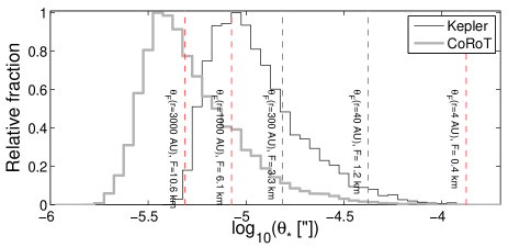
Figure 1.— Approximate stellar angular radius distributions for Kepler (black line) and CoRoT (gray line). The vertical red dashed lines represent the Fresnel radii at selected distances (see labels) where $\lambda=5000$ Å.

3.2. Relative velocity distribution

Given the unit vector in the direction of a target $\hat{r}$, the speed of the observer relative to the occulting object $v$, and the heliocentric velocity unit vector of the observer $\hat{v}$, the approximate relative velocity, of an observer in an Earth trailing orbit, projected on the plane perpendicular to $\hat{r}$ is

$$v_{{\rm rel}}=v\sqrt{1-(\hat{v}\cdot\hat{r})^{2}}\cong v_{\oplus}\sqrt{1-\cos^{2}{(\lambda-\lambda_{\oplus})}\cos^{2}{\beta}},$$ (2)

where $\lambda$ and $\beta$ are the ecliptic longitude and latitude of the observed star, $\lambda_{\oplus}$ is the ecliptic longitude (as measured from the Sun) of the observer, and $v_{\oplus}\approx 29.8$ km s^-1 is the heliocentric speed of the observer. Finally, assuming circular orbit (i.e., the probability distribution of $\lambda_{\oplus}$ is uniform) the probability distribution of $v_{{\rm rel}}$ is $P_{v_{{\rm rel}}}=\frac{d\lambda_{\oplus}}{dv_{{\rm rel}}}$.

3.3. Ecliptic latitude distribution

The Oort Cloud is predicted to have a roughly spherical shape. However, the Kuiper Belt and the asteroids main belt are concentrated toward the ecliptic plane. Using the inclination distribution of KBOs estimated by Elliot et al. (2005) the expectation probability to find a KBO at an ecliptic latitude of $\mathrel{\raise 1.29167pt\hbox{$>$}\mkern-14.0mu\lower 2.58334pt\hbox{$\sim$}}66^{\circ}$ is about $f_{\epsilon}\sim 6\times 10^{-6}$ times smaller than that at the ecliptic. This relative probability was estimated by convolving the inclination probability distribution of KBOs with the ecliptic latitude distribution for a given inclination (i.e., Elliot et al. 2005 eqs. 40 and 34, respectively). We note, however, that this number is highly uncertain.

3.4. Rate estimates

To estimate the rate of occultation events we integrate the appropriate formulas in Table 2 over $v_{{\rm rel}}$, $r$, $\theta_{*}$ and $S$ co-distributions. For each combination of parameters we integrate over the most appropriate occultation channel (i.e., cases A–E). In Table 3 we present the estimated rates predicted for Kepler and CoRoT for the Oort Cloud (upper block), Kuiper Belt (middle block), and main belt (lower block) object occultations. The predicted rate for Oort Cloud objects in Table 3 in case of $q=3.5$ and $r_{{\rm min}}=3000$ AU is lower by about an order of magnitude compared to the pre-factors in Table 2. This is mostly because Table 2 is normalized for all objects being at $r=3000$ AU while in Table 3 the same number of objects is spread between $r_{{\rm min}}$ and $r_{{\rm max}}$, with a spatial density distribution proportional to $r^{-3.5}$.

Table 3Approximate occultation rates

Parameters			Rates ($\tau=3$ yr)
			Kepler	CoRoT
$N_{>1\,{\rm km}}$	$r_{{\rm min}}$	$q$	$f_{\epsilon}=6\times 10^{-6}$	$f_{\epsilon}=1$
[deg-2]	[AU]		$N_{*}=10^{5}$, $\beta\approx 66^{\circ}$	$N_{*}=10^{4}$, $\beta\approx 0^{\circ}$
$2.4\times 10^{8}$	$3000$	$3.0$	30	0.1
$2.4\times 10^{8}$	$3000$	$3.5$	8	$4\times 10^{-3}$
$2.4\times 10^{8}$	$3000$	$4.5$	0.7	$1\times 10^{-5}$
$2.4\times 10^{8}$	$1000$	$3.5$	60	0.03
$2.4\times 10^{8}$	$5000$	$3.5$	3	$2\times 10^{-3}$
$1.1\times 10^{4}f_{\epsilon}$	$40$	$3.0$	$2\times 10^{-4}$	$3\times 10^{-3}$
$7.3\times 10^{4}f_{\epsilon}$	$40$	$3.5$	$5\times 10^{-4}$	$4\times 10^{-3}$
$4.9\times 10^{5}f_{\epsilon}$	$40$	$4.0$	$5\times 10^{-3}$	$0.02$
$47f_{\epsilon}$	$4$	$2.3$	$1\times 10^{-4}$	0.2

Note. — The first block refers to Oort Cloud objects assuming $r_{{\rm max}}=50000$ AU, $\alpha=-3.5$. The second block refers to KBOs assuming $r_{{\rm max}}=40$ AU. The third block refers to main belt asteroids assuming $r_{{\rm max}}=4$ AU. The cumulative surface density of KBOs near the break radius, $R_{{\rm break}}\approx 45$ km, is 5.4 deg^-2 at the ecliptic (Fuentes et al. 2009). Therefore, at the ecliptic we adopt for KBOs, $N_{>1\,{\rm km}}$ of $1.1\times 10^{4}$, $7.3\times 10^{4}$, and $4.9\times 10^{5}$ deg^-2, for $q=$3, 3.5, and 4, respectively. We note that these values are consistent with the findings of Schlichting et al. (2009). $N_{{>1\,\rm km}}$ and $q$ for the main belt are taken from Ivezić et al. (2001). We set the ecliptic latitude surface density correction $f_{\epsilon}$ to $6\times 10^{-6}$ and 1 for $\beta\approx 66^{\circ}$ and $\beta\approx 0$, respectively, for both KBOs and main belt asteroids. In all the cases we assume eight sigma detection threshold (i.e., $n=8$).

These rate estimates suggest that if our current ’best guess’ regarding the properties of the Oort Cloud are correct, then it may be detectable by Kepler. Regardless, Kepler will be able to put the best constraint (so far) on the content of the Oort Cloud. We note that the rate estimates in Table 3 are an approximation to the actual rate. This is mainly because our formulas represent asymptotic approximations, while in some cases two out of the three angular scales, $\theta_{{\rm obj}}$, $\theta_{{\rm F}}$, $\theta_{*}$, maybe be similar.

4. Validation and degeneracy removal

Contrary to transits and grazing transits by extra-solar planets, solar system occultations will appear in a single photometric measurement and they happen only once. Therefore, verification of each event by itself will require a thorough understanding of the noise properties of the photometer. Kepler will have about $1.5\times 10^{10}$ 15-min independent photometric measurements. Assuming purely Gaussian noise, the 8-$\sigma$ detection threshold we adopted corresponds to a probability of $\sim 10^{-15}$. However, even small deviations from a Gaussian noise may impair our confidence in the astrophysical nature of the events.

Here we present two tests that can be used to check if the occultations signature are due to real events or due to some sort of uncharacterized noise. In addition, these tests can be used to statistically measure $q$ and to distinguish between Oort Cloud objects and KBOs.

The occultation rate depends on the relative velocity $v_{{\rm rel}}$, with a somewhat different dependency in each regime. Therefore, if a large number of occultations are detected, a simple sanity test is to look for the dependency of the events rate on $v_{{\rm rel}}$. We note that since Kepler is observing at high ecliptic latitude the $v_{{\rm rel}}$ modulation will be small (Eq. 2) compared to the maximal modulation which will be seen by an instrument observing the ecliptic. Moreover, in all the cases (A–E), the function $N_{{\rm ev}}$ depends on $q$. Therefore, the amplitude of the modulation is related to $q$ and the occultation type (i.e., A–E). Knowing the occultation regime (see below), we can measure $q$ (i.e., removing the degeneracy between $q$ and $N_{{\rm ev}}$).

Furthermore, as shown in Table 2 the occultations rate depends on $S$, which depends on the stellar magnitude and on $\theta_{*}$, which in turn is a function of the star magnitude and effective temperature. We expect bright and angularly small stars to have higher chance of producing detectable occultations. Moreover, this dependency is different for the various occultation cases. This can be used to further test the nature of the occultations, by comparing the distribution of magnitudes and effective temperatures of the stars showing occultations to those of the entire observed stellar population. Most importantly, for a Kepler-like observatory, KBO occultations will be mostly in the diffractive regime, while Oort Cloud object occultations will be in the geometric regime (Fig. 1). Therefore, the magnitude and $\theta_{*}$ of occulted stars by KBOs and Oort Cloud objects will follow different co-distributions. Therefore, we can statistically distinguish between Oort Cloud and KBO occultation events. However, quantifying these effects and estimating the number of occultations needed to carry out the suggested analysis requires a more realistic estimate of the events rate (i.e., using full numerical integration of light curves) and a full exploration of the parameters space.

To summarize, we show that Kepler and similar space missions can detect deca-kilometer objects in the Oort Cloud. We present statistical methods to verify that the occultations are real rather than due to uncharacterized noise. In addition we suggest that it will be possible to statistically measure their size distribution ($q$), and the dominant occultation regime, and therefore differentiate between Oort cloud objects and KBOs.

Considering Kepler capabilities and reasonable Oort Cloud parameters, we find that Kepler may detect 0 to $\sim 10^{2}$ stellar occultations by Oort Cloud objects. We find that Kepler is unlikely to detect Kuiper Belt objects (mainly because of its high ecliptic latitude pointing). Moreover, CoRoT is unlikely to detect Kuiper Belt or Oort Cloud objects. However, the exact properties of the Oort Cloud and the Kuiper Belt are not well known. Therefore, such searches are warranted.

The analytical treatment we present in this paper is useful in order to maximize the efficiency of existing (and future, e.g., PLATO) experiments to detect trans Neptunian objects. However, this treatment is accurate only in the asymptotic cases, and numerical calculations are needed in order to give more precise predictions.

References

- Bailey (1976) Bailey, M. E. 1976, Nature, 259, 290
- Bailey (1983) Bailey, M. E. 1983, MNRAS, 204, 603
- Bailey & Stagg (1988) Bailey, M. E., & Stagg, C. R. 1988, MNRAS, 235, 1
- Bernstein et al. (2004) Bernstein, G. M., Trilling, D. E., Allen, R. L., Brown, M. E., Holman, M., & Malhotra, R. 2004, AJ, 128, 1364
- Bianco et al. (2009) Bianco, F. B., Protopapas, P., McLeod, B. A., Alcock, C. R., Holman, M. J., & Lehner, M. J. 2009, arXiv:0903.3036
- Brasser et al. (2006) Brasser, R., Duncan, M. J., & Levison, H. F. 2006, Icarus, 184, 59
- Brasser et al. (2008) Brasser, R., Duncan, M. J., & Levison, H. F. 2008, Icarus, 196, 274
- Chang et al. (2006) Chang, H.-K., King, S.-K., Liang, J.-S., Wu, P.-S., Lin, L. C.-C., & Chiu, J.-L. 2006, Nature, 442, 660
- Chang et al. (2007) Chang, H.-K., Liang, J.-S., Liu, C.-Y., & King, S.-K. 2007, MNRAS, 378, 1287
- Dones et al. (2004) Dones, L., Weissman, P. R., Levison, H. F., & Duncan, M. J. 2004, Star Formation in the Interstellar Medium: In Honor of David Hollenbach, 323, 371
- Duncan et al. (1987) Duncan, M., Quinn, T., & Tremaine, S. 1987, AJ, 94, 1330
- Elliot et al. (2005) Elliot, J. L., et al. 2005, AJ, 129, 1117
- Farinella & Davis (1996) Farinella, P., & Davis, D. R. 1996, Science, 273, 938
- Fernández (1997) Fernández, J. A. 1997, Icarus, 129, 106
- Fernández & Brunini (2000) Fernández, J. A., & Brunini, A. 2000, Icarus, 145, 580
- Fuentes & Holman (2008) Fuentes, C. I., & Holman, M. J. 2008, AJ, 136, 83
- Gaudi & Bloom (2005) Gaudi, B. S., & Bloom, J. S. 2005, ApJ, 635, 711
- Goldreich et al. (2004) Goldreich, P., Lithwick, Y., & Sari, R. 2004, ApJ, 614, 497
- Heisler & Tremaine (1986) Heisler, J., & Tremaine, S. 1986, Icarus, 65, 13
- Heisler (1990) Heisler, J. 1990, Icarus, 88, 104
- Hills (1981) Hills, J. G. 1981, AJ, 86, 1730
- Ivezić et al. (2001) Ivezić, Ž., et al. 2001, AJ, 122, 2749
- Lasker et al. (2008) Lasker, B. M., et al. 2008, AJ, 136, 735
- Lehner et al. (2009) Lehner, M. J., et al. 2009, PASP, 121, 138
- Moro & Munari (2000) Moro, D., & Munari, U. 2000, A&AS, 147, 361
- Nihei et al. (2007) Nihei, T. C., Lehner, M. J., Bianco, F. B., King, S.-K., Giammarco, J. M., & Alcock, C. 2007, AJ, 134, 1596
- Ofek (2008) Ofek, E. O. 2008, PASP, 120, 1128
- Oort (1950) Oort, J. H. 1950, Bull. Astron. Inst. Netherlands, 11, 91
- Pan & Sari (2005) Pan, M., & Sari, R. 2005, Icarus, 173, 342
- Poznanski et al. (2002) Poznanski, D., Gal-Yam, A., Maoz, D., Filippenko, A. V., Leonard, D. C., & Matheson, T. 2002, PASP, 114, 833
- Roques et al. (1987) Roques, F., Moncuquet, M., & Sicardy, B. 1987, AJ, 93, 1549
- Roques et al. (2006) Roques, F., et al. 2006, AJ, 132, 819
- Schlichting et al. (2010) Schlichting, H. E., Ofek, E. O., Wenz, M., Sari, R., Gal-Yam, A., Livio, M., Nelan, E., Zucker, S. 2010, Nature in press
- Weissman (1996) Weissman, P. R. 1996, Completing the Inventory of the Solar System, 107, 265