Discerning The Form of the Dense Core Mass Function

Abstract

We investigate the ability to discern between lognormal and powerlaw forms for the observed mass function of dense cores in star forming regions. After testing our fitting, goodness-of-fit, and model selection procedures on simulated data, we apply our analysis to 14 datasets from the literature. Whether the core mass function has a powerlaw tail or whether it follows a pure lognormal form cannot be distinguished from current data. From our simulations it is estimated that datasets from uniform surveys containing more than $\approx 500$ cores with a completeness limit below the peak of the mass distribution are needed to definitively discern between these two functional forms. We also conclude that the width of the core mass function may be more reliably estimated than the powerlaw index of the high mass tail and that the width may also be a more useful parameter in comparing with the stellar initial mass function to deduce the statistical evolution of dense cores into stars.

1. Background

Stars form from dense cores of molecular gas and dust with sizes $\approx 0.1$ pc, masses between $\approx 0.5$ and 50 $M_{\odot}$, and densities $\gtrsim 10^{4}$ cm^-3 (see, e.g., Bergin & Tafalla 2007). Therefore the relationship between mass distributions of dense cores in star forming regions (core mass function, or CMF) and the stellar initial mass function (IMF) contains information regarding how observed samples of cores evolve into stars. The observational similarity between the CMF and the IMF was first put forth by Motte et al. (1998), and since this time many other samples of dense cores have been presented in this context (e.g., Simpson et al. 2008; Enoch et al. 2008; Alves et al. 2007; Nutter & Ward-Thompson 2007; Stanke et al. 2006; Johnstone et al. 2001). The qualitative similarity between the CMF and the IMF offers support for the accepted idea that stars form from dense cores (e.g. Lada et al. 2008). But what can we learn about the star formation process from this observed similarity?

In a recent paper, we presented a series of numerical experiments evolving distributions of cores into stellar IMFs (Swift & Williams 2008). We find that a given CMF evolved according to different evolutionary pathways produces variations in the resultant IMF that are insignificant in relation to the errors inherent in current samples of dense cores. Our results show that the form of the CMF in relation to the IMF indeed contains vital clues to the star formation process, but highlight the difficulty in deducing how observed samples of cores evolve into stars based solely on the shapes of these distributions.

The central limit theorem applied to isothermal turbulence naturally predicts a lognormal probability distribution in density (Larson 1973; Zinnecker 1984; Adams & Fatuzzo 1996) that has been produced in computer simulations (e.g., Vazquez-Semadeni 1994; Nordlund & Padoan 1999; Klessen 2001). Extensive surveys of nearby star-forming regions have also shown a CMF shape consistent with a lognormal form (e.g., Enoch et al. 2008; Stanke et al. 2006).

However, observed CMFs are typically characterized by one or more powerlaws. While the use of a powerlaw form to fit observed CMFs has never been rigorously justified, this form is assumed based on its versatility and the expected similarity between the CMF and the IMF (e.g., Motte et al. 1998). Recent data show that this apparent powerlaw behavior does not extend to very low masses but displays a turnover or break below a few $M_{\odot}$ (Alves et al. 2007). Motivated by the observational similarity of the CMF and the IMF, theories have been recently developed describing physical scenarios that may produce a powerlaw distribution of molecular core masses that turns over toward low-masses (Padoan & Nordlund 2002; Shu et al. 2004; Hennebelle & Chabrier 2008).

To understand how, or if, dense molecular cores produce the full spectrum of stellar masses, it is essential to understand the probability distribution function (PDF) from which the CMF is drawn. If the parent distribution has a powerlaw tail extending to high masses, this would support the idea that stellar mass is almost entirely determined in the molecular cloud phase (e.g., Alves et al. 2007). If observed mass distributions of cores are found to be drawn from a purely lognormal PDF, the origin of the powerlaw distribution of stellar masses will remain an open question. A lognormal CMF would disfavor the idea that massive stars form directly from massive cores (such as Krumholz et al. 2009), and may imply that massive stars form through mechanisms distinct from low-mass stars (e.g., Bonnell et al. 2004). Distinguishing between these two forms is complicated by the difficulty in measuring the CMF over large dynamic ranges and the fact that lognormal and powerlaw forms can look quite similar over limited mass ranges.

In 2006, Reid & Wilson concluded that observed CMFs are consistent with being drawn from the same parent distribution and that this parent distribution is consistent with the IMF. However, the results of their Kolmogorov-Smirnov (KS) tests applied to the median normalized CMFs suggest that the CMFs are indistinguishable while their goodness-of-fit statistic based on $\chi^{2}$ suggest that different core samples may have different preferred forms. Given these ambiguities and the fact that the KS test is somewhat compromised when applied to two distributions with normalized medians, we revisit the topic of discerning the form of the parent distribution to the CMF with a new approach. A renewed interest in this subject is motivated by new instruments coming online (e.g., Herschel, SCUBA2, ALMA) and surveys that will provide large, uniform samples of carefully selected cores.

In § 2 we outline our analysis strategy and then test our procedures on simulated data in § 3. The application of our procedures to 14 state-of-the-art datasets of dense cores in star-forming regions is presented in § 4, and we close with a discussion of these results in § 5 that includes suggestions for future observations.

2. Data Analysis

The goals of our data analysis are to (1) find the best fit parameters for lognormal and powerlaw models given the data, (2) assess whether or not a given model adequately describes the data, (3) select either the lognormal or powerlaw model as the preferred model, and (4) compute the confidence in that selection. The following sub-sections outline the details of each step used to achieve these goals. All procedures were written in the Interactive Data Language.

2.1. The Models

The two models we choose to differentiate in our analysis are motivated in § 1 and are described by probability distribution functions (PDFs) of powerlaw and lognormal form. The powerlaw PDF is given by

$$p_{\rm pl}(m)=C_{\rm pl}m^{-\alpha}$$ (1)

for $m\geq m_{0}$. The normalization constant is given by

$$C_{\rm pl}=(\alpha-1)m_{0}^{\alpha-1}$$

where $m_{0}$ signifies the break or “turnover” below which the distribution does not follow powerlaw behavior.

The lognormal PDF is given by

$$p_{\rm ln}(m)=\frac{C_{\rm ln}}{m}\exp\left[-\frac{(\ln m-\mu)^{2}.}{2\sigma^{2}}\right]$$ (2)

with the normalization constant

$$C_{\rm ln}=\sqrt{\frac{2}{\pi\sigma^{2}}}\left[{\rm erfc}\left(\frac{\ln m_{\rm lim}-\mu}{\sigma\sqrt{2}}\right)\right]$$

where the characteristic mass $m_{\rm c}=e^{\mu}$ and $m_{\rm lim}$ is the minimum mass of the distribution, analogous to an observational completeness limit.

2.2. Fitting

To avoid the dangers inherent in fitting data using regression models arising from, e.g., data binning (Rosolowsky 2005), we use the method of maximum likelihood to estimate the model parameters for both simulated and real data (see Clauset et al. 2007).

The best estimate of the powerlaw index for data with values above $m_{0}$ is found analytically by maximizing the log-likelihood:

$$\hat{\alpha}=1+n\left[\sum_{i=1}^{n}\ln\left(\frac{m_{i}}{m_{0}}\right)\right]^{-1}$$ (3)

where $n$ is the number of data with $m\geq m_{0}$. Hatted quantities will signify the best fit parameters throughout the text. The value of $m_{0}$ is also unknown and is found by minimizing the KS statistic between the best fit model and the data as a function of $m_{0}$ (Clauset et al. 2007, § 3.3).

The likelihood for the distribution in Equation 2 cannot be maximized analytically. Therefore, we numerically maximize the likelihood for the lognormal model as a function of $\sigma$ and $\mu$ using Powell’s method (Press et al. 2007).

2.3. Goodness-of-fit

Once the data are fit, we calculate the KS statistic between the best fit model and the data as a proxy for goodness-of-fit. When one or more parameters of a model are determined from data, the probability value for the KS statistic, $p_{\rm KS}$, can no longer be found directly from the KS probability distribution (Lilliefors 1967). We therefore calculate $p_{\rm KS}$ by relating the KS statistic to the distribution of values generated from 5000 parametric bootstrap realizations (Press et al. 2007; Babu & Feigelson 2006; Clauset et al. 2007).

The value of $p_{\rm KS}$ represents the probability of getting a fit worse than the original given the model and the PDF of the distribution. Low values of $p_{\rm KS}$, typically below 0.1 or 0.05, are a flag for a given model being an inadequate description of the data.

2.4. Model Selection

There are several approaches to selecting between models. Bayesian model selection compares the evidence of each model computed as an integral over all free parameters of the probability density, i.e., the likelihood function. One of our free parameters, $m_{0}$, determines the number of data points to be considered by the models thus adding a difficult complexity to this approach. Instead we use the likelihood ratio test, a similar approach that compares the peak probability densities of the models. Taking the log of this ratio we obtain the parameter

$$\mathcal{R}=\sum_{i=1}^{n}\left[\ln p_{\rm pl}(m_{i})-\ln p_{\rm ln}(m_{i})\right]$$ (4)

where positive values of $\mathcal{R}$ favor the powerlaw model and negative values favor the lognormal model.

Our two models each have two parameters—$m_{0}$ and $\alpha$ for the powerlaw model, and $\mu$ and $\sigma$ for the lognormal model. Therefore we do not expect there to be biases introduced into this method due to different levels of complexity in the models. An additional benefit to using this test is that the significance of ${\rm sgn}(\mathcal{R})$ can be assessed by generating a distribution of $\mathcal{R}$ values through bootstrap resampling of the data (for real data) or the PDF (for simulated data). The fraction of $\mathcal{R}$ values having the same sign as the original value is designated $C_{\mathcal{R}}$, the confidence level of the likelihood ratio.

3. Application to Simulated Data

To ascertain how well our procedures discriminate between powerlaw and lognormal distributions, we have carried out our analysis on a large number of simulated datasets. These simulations quantify how sensitively the model selection process depends on the sample size and $m_{\rm lim}$.

Distributions with $N_{\rm C}$ samples above a completeness limit of $m_{\rm lim}$ for $N_{\rm C}=50\times 2^{n}$ ($n=0,1,2,...,8$) and $m_{\rm lim}=$ 0.1, 0.5, and 1.0 $M_{\odot}$ are drawn from the PDFs of § 2.1. For powerlaw data, we draw from the distribution in Equation 1 for masses above $m_{0}$ while for masses between $m_{\rm lim}$ and $m_{0}$ we draw from Equation 2. The powerlaw data are drawn such that the parent distribution is smooth and continuous at $m_{0}=\mu-\sigma^{2}(1-\alpha)$. Lognormal data are drawn from the distribution in Equation 2. For each sample size, $N_{\rm c}$, and completeness limit, $m_{\rm lim}$, 5000 distributions are realized and fit according to the procedures outlined in § 2.

We use values $\sigma=1.0$ and $\mu=0$ for all simulated data, consistent with CMFs measured in nearby star-forming regions (Enoch et al. 2008; Stanke et al. 2006). For powerlaw data we use $\alpha=2.5$, close to the Salpeter value of 2.35 (Salpeter 1955) and also consistent with data from the literature (Reid & Wilson 2006b, also see Table 2).

3.1. Likelihood Ratio Test

Figure 1 displays $C_{\mathcal{R}}$ as a function of $N_{\rm C}$ given different values of $m_{\rm lim}$. The solid lines in the figure represent the confidence with which the underlying powerlaw form to the PDF can be discerned from a lognormal form. The confidence is an increasing function of $N_{\rm C}$ and a decreasing function of $m_{\rm lim}$ expressed here as the fraction of the characteristic mass of the distribution, $m_{\rm lim}/m_{\rm c}$. The dependency on $N_{\rm C}$ is expected and reflects the increasing amount of information available to the likelihood ratio test. The dependency on $m_{\rm lim}$ arises because a lognormal form can closely approach a powerlaw form over a limited range for large negative values of $\hat{\mu}$ and large positive values of $\hat{\sigma}$. Therefore, as more data are included below $m_{0}$ stronger constraints can be placed on the values of $\hat{\mu}$ and $\hat{\sigma}$ thereby creating a larger discrepancy between a lognormal model and the high mass tail of the simulated data. We find that a lognormal form to the CMF can be ruled out at the 95% confidence level for a survey of intermediate sensitivity and sample sizes greater than $\approx 500$.

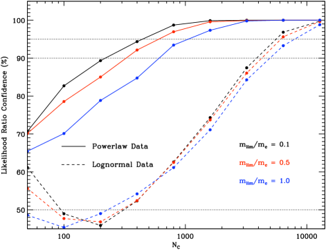
Figure 1.— The confidence with which the likelihood ratio test can discern between a powerlaw and lognormal model for data generated from a powerlaw (solid lines) and lognormal (dashed lines) probability distribution function as a function of the sample size, $N_{\rm C}$. Data with completeness limits of 0.1, 0.5, and 1.0 times the characteristic mass are shown in black, red, and blue, respectively.

The dashed lines in Figure 1 represent the confidence level with which a pure lognormal form to the PDF can be distinguished from a one with a powerlaw tail. We see that these curves are monotonically increasing for $N_{\rm C}\gtrsim 100$. The upturn in the lognormal data curves at low $N_{\rm C}$ is due to the effects of fitting a powerlaw to a small number of data points. As $N_{\rm C}$ increases, so do the best fit values, $\hat{m_{0}}$ and $\hat{\alpha}$, thereby making a distinction between models more difficult than for the case of powerlaw data. If $m_{0}$ is forced to lie at some fraction of $m_{\rm c}$, then results similar to the a powerlaw data (solid lines) are obtained. The dependency of $C_{\mathcal{R}}$ on $m_{\rm lim}$ is weaker for the lognormal data than the powerlaw data since lower values of $m_{\rm lim}$ produce only slightly better lognormal fits.

3.2. Goodness-of-fit Test

Figure 2 shows the average value of $p_{\rm KS}$ as a function of $N_{\rm C}$ generated by fitting the incorrect model to the simulated data. For both the powerlaw and lognormal data, the incorrect model produces poorer fits as the sample size increases. Similar to the likelihood ratio test, it is more difficult to rule out a powerlaw model from lognormal data. However, the discrepancy between the critical values of $N_{\rm C}$ is smaller using this test.

For powerlaw data, $\langle p_{\rm KS}\rangle$ is a decreasing function of $m_{\rm lim}$. This dependency comes about since the KS test is most sensitive to the median of a distribution and the powerlaw and lognormal models have median values that become closer as $m_{\rm lim}$ decreases. For lognormal data, $\langle p_{\rm KS}\rangle$ is not a monotonic function of $m_{\rm lim}$ for all values of $N_{\rm C}$.

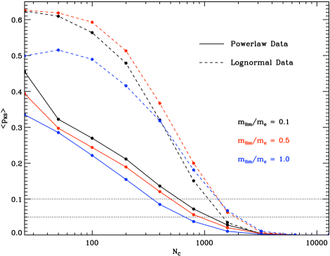
Figure 2.— The average KS probability resulting from fitting a lognormal model to powerlaw data (solid lines) or a powerlaw model to lognormal data (dashed lines). Color conventions are the same as in Figure 1.

It may be expected that the curves of $\langle p_{\rm KS}\rangle$ should approach 0.5 as $N_{\rm C}\rightarrow 0$, meaning that the two models are indistinguishable for small sample sizes. However, it can be seen that the curves representing lognormal data (dashed lines) overshoot this value for $N_{\rm C}$ between about 50 and 200. As in § 3.1, this results from fitting a powerlaw to a small number of samples and represents a bias for lognormal data to look marginally more like a powerlaw for $N_{\rm C}$ in this range according to our goodness-of-fit test.

From these simulations it can be concluded that fitting a powerlaw model to lognormal data or conversely a lognormal model to powerlaw data will consistently yield very low values of $p_{\rm KS}$ for $N_{\rm C}$ greater than several hundred to a thousand.

4. Application to Literature Data

Table 4 lists the 14 datasets to which we apply the analysis of § 2 along with their descriptive parameters. Various techniques are used to observationally identify the cores in these datasets. The most common technique is the use of threshold contouring (e.g., Alves et al. 2007), though gaussian fitting (e.g., Nutter & Ward-Thompson 2007) and wavelet decomposition (e.g., Motte et al. 1998) are also used.

The results of our fitting procedures, goodness-of-fit tests, and model selection techniques are displayed in Table 2. For a majority of the datasets, neither a lognormal form nor a powerlaw provide a significantly better description of the data. Five datasets out of 14 have values of $p_{\rm KS}$ and $C_{\mathcal{R}}$ that are potentially significant. These values are underlined in the table for emphasis.

Datasets 3, 11 and 14 disfavor a powerlaw model due to a very low $p_{\rm KS}$ value while showing various levels of support for a lognormal model in the likelihood ratio. Dataset 12 disfavors a lognormal form in the $p_{\rm KS}$ statistic while showing moderate support for a powerlaw form in the likelihood ratio test. Dataset 6 is not adequately fit by either model.

Table 1Literature Data

Dataset ID	Region	$N_{\rm tot}$	$m_{\rm lim}$	$N_{C}$	Ref.
1	Pipe Nebula	159	1.0	73	1
2	Pipe Nebula	134	0.6	81	2
3	Bolocam Cores (SL)	108	0.8	69	3
4	Bolocam Cores (PS)	92	0.8	45	3
5	Bolocam Cores (All)	200	0.8	114	3
6	$\rho$ Ophiuchus	55	0.1	40	4
7	$\rho$ Ophiuchus	143	0.1	120	5
8	$\rho$ Ophiuchus	62	0.1	51	6
9	Orion A	172	0.3	170	7
10	Orion	203	1.0	149	8,9,10
11	M17	121	3.0	108	11
12	NGC 7538	77	15	45	12
13	Cygnus X	129	5.3	125	13
14	NGC 6334	181	32	131	14

References. — (1) Alves et al. (2007), (2) Rathborne et al. (2009), (3) Enoch et al. (2008), (4) Johnstone et al. (2000), (5) Stanke et al. (2006), (6) Motte et al. (1998), (7) Nutter & Ward-Thompson (2007), (8) Johnstone et al. (2001), (9)Johnstone et al. (2006), (10) Johnstone & Bally (2006), (11) Reid & Wilson (2006a), (12) Reid & Wilson (2005), (13) Motte et al. (2007), (14) Muñoz et al. (2007)

Table 2Literature Analysis Results

	Powerlaw Fit				Lognormal Fit
Dataset ID	$\hat{\alpha}$	$\hat{m_{0}}$	$p_{KS}$	$N_{\rm tail}$	$\hat{\mu}$	$\hat{\sigma}$	$p_{KS}$		$m_{\rm lim}/m_{\rm c}$	$\mathcal{R}$	$C_{\mathcal{R}}$
1	$2.9^{+0.6}_{-0.5}$	$2.5^{+0.04}_{-1.1}$	0.75	27	$-0.1^{+0.6}_{-2.6}$	$1.1^{+0.8}_{-0.3}$	0.90		1.1	PL	76%
2	$3.0^{+0.6}_{-0.5}$	$2.4^{+0.3}_{-1.3}$	0.43	30	$0.2^{+0.3}_{-0.6}$	$1.0^{+0.3}_{-0.2}$	0.51		0.5	PL	71%
3	$2.7^{+0.3}_{-0.3}$	$0.9^{+0.7}_{-0.1}$	0.00	65	$0.0^{+0.3}_{-0.8}$	$0.7^{+0.3}_{-0.2}$	0.42		0.8	LN	91%
4	$3.4^{+0.5}_{-0.5}$	$2.5^{+0.1}_{-0.9}$	0.72	22	$0.7^{+0.2}_{-0.4}$	$0.7^{+0.3}_{-0.1}$	0.68		0.4	PL	68%
5	$4.1^{+1.0}_{-0.8}$	$2.7^{+0.1}_{-1.5}$	0.32	28	$0.2^{+0.2}_{-0.5}$	$0.8^{+0.2}_{-0.1}$	0.54		0.7	PL	60%
6	$1.9^{+0.2}_{-0.2}$	$0.2^{+0.5}_{-0.01}$	0.00	37	$-0.9^{+0.2}_{-0.3}$	$0.9^{+0.3}_{-0.2}$	0.06		0.2	LN	77%
7	$2.8^{+0.5}_{-0.4}$	$0.6^{+0.04}_{-0.2}$	0.85	43	$-1.1^{+0.2}_{-0.3}$	$1.0^{+0.2}_{-0.1}$	0.45		0.3	PL	85%
8	$2.0^{+0.2}_{-0.2}$	$0.1^{+0.1}_{-0.02}$	0.15	46	$-4.1^{+2.1}_{-2.0}$	$1.9^{+0.8}_{-0.7}$	0.20		5.9	LN	69%
9	$1.9^{+0.2}_{-0.2}$	$6.4^{+1.8}_{-5.3}$	0.67	37	$-5.4^{+1.4}_{-3.9}$	$3.4^{+1.1}_{-0.5}$	0.94		200	PL	56%
10	$2.7^{+0.3}_{-0.3}$	$3.1^{+2.4}_{-0.6}$	0.21	69	$0.7^{+0.2}_{-0.4}$	$1.0^{+0.2}_{-0.1}$	0.45		0.5	PL	68%
11	$2.1^{+0.2}_{-0.2}$	$14^{+6}_{-8}$	0.00	59	$2.6^{+0.2}_{-0.3}$	$1.1^{+0.2}_{-0.2}$	0.59		0.2	LN	90%
12	$2.1^{+0.4}_{-0.32}$	$68^{+4}_{-45}$	0.57	22	$2.7^{+1.1}_{-3.0}$	$1.9^{+1.3}_{-0.6}$	0.07		1.0	PL	84%
13	$2.1^{+0.2}_{-0.2}$	$21^{+5}_{-5}$	0.66	65	$2.7^{+0.3}_{-0.5}$	$1.3^{+0.3}_{-0.2}$	0.14		2.2	PL	83%
14	$1.7^{+0.1}_{-0.1}$	$47^{+41}_{-13}$	0.09	111	$2.6^{+1.3}_{-3.9}$	$2.2^{+1.2}_{-0.5}$	0.74		2.3	LN	74%

5. Discussion

5.1. Does the CMF Have a Powerlaw Tail?

Ambiguous results for more than 60% of the datasets and conflicting results for the remaining $\sim 40$% emphasize the difficulty in discerning the form of the CMF. Given the results in Table 2, we conclude that a pure lognormal PDF and a PDF with a powerlaw tail cannot be distinguished from current core datasets. Furthermore, neither the existence of a powerlaw tail to the CMF nor the uniformity of the CMF from region to region are evident.

It is not clear to what degree systematic differences in each dataset—differing observational techniques, physical resolution, filtering, core identification algorithms, and parameters used in deriving core mass (e.g., $\kappa_{\nu}$)—contribute to the variations seen from dataset to dataset, and it is possible that a uniform re-analysis of the datasets could reveal a more definitive relationship between the shapes of the CMFs. Also, the free parameters are unconstrained in our fitting procedures, and in some cases this leads to fits that could be seen as unreasonable (e.g., the low values of $\hat{\mu}$ for datasets 8 and 9). Judicious constraints on the fitting parameters could therefore lead to more decisive results.

However, our conclusions are consistent with the results from § 3. The literature datasets of Table 4 have $N_{\rm C}\lesssim 150$ while the results of § 3 suggest that more than $\approx 500$ samples are needed to definitively discern between these two models. These results highlight the need for larger, uniform survey data to produce a statistically significant result regarding the functional form of the CMF.

5.2. Comparing the CMF to the IMF

The utility in analyzing the form of the CMF is in its relation to the stellar IMF to address the question of how the final mass of a star is determined. The similarity of the CMF to the IMF has inspired the idea that the masses of stars are determined via the fragmentation of dense molecular gas in the Galaxy. It seems as though this must be true at least in part since it is known that stars form in dense, self-shielded molecular gas. However, whether or not the mass distributions of molecular cores observed in star-forming regions will accurately represent the mass distribution of stars to form from them is still debatable.

It was shown by Swift & Williams (2008) that different evolutionary pathways from cores to stars produce variations in the form of the resultant IMF. The powerlaw slope was shown to be quite robust except under the most extreme evolutionary scenarios due to the scale-free nature of powerlaw distributions. The width however was shown to be a more sensitive indicator of core evolution. Given the small dynamic range over which the CMF can be measured in nearby star-forming regions, we emphasize the importance of obtaining a sound measurement of $\sigma$ in survey data as this parameter may be more powerful than $\alpha$ in constraining how observed distributions of cores evolve into stars.

The width of the IMF has been measured to be between 0.3 and 0.7 dex (Miller & Scalo 1979; Chabrier 2003; Bochanski et al. 2009). The measured values of $\hat{\sigma}$ in Table 2 tend to be higher than this, approximately between 0.7 and 2. If this were confirmed to be the case in a more sensitive, uniform survey, this would indicate that an additional mass preference occurs in later stages of gravitational collapse likely through fragmentation into several stars at or near the local Jeans mass.

5.3. Bettering Our Understanding of the CMF

It is a difficult task to automate the identification of large numbers of pre-stellar molecular cores in star-forming regions, and there is no consensus on how to define a core observationally. However, methods are currently being improved (Kainulainen et al. 2009; Pineda et al. 2009) and new strategies are being developed (e.g., Rosolowsky et al. 2008). It has been recently shown that the physical characteristics of cores (e.g., Rathborne et al. 2009), the potential variability of core lifetimes (Clark et al. 2007) as well as the effects of statistical errors (e.g., Koen & Kondlo 2009; Rosolowsky 2005) are also important to consider when interpreting observed CMFs.

From this work, we present three new suggestions aimed to help maximize the utility of future surveys of dense cores in star-forming regions. One, is that sample sizes of greater than $\approx 500$ above the completeness limit should be sought so that a lognormal and powerlaw tail to the CMF can be discerned. The second suggestion is that the survey should be as uniform as possible such that systematic errors can be minimized. The third suggestion is that a sensitivity limit of better than one half of the peak mass of the distribution is desirable such that the width of the CMF can be reliably determined and compared to the width of the IMF.

A survey such as the Gould’s Belt Legacy Survey to be conducted with SCUBA2 on the James Clerk Maxwell Telescope may very well reach these goals, and the value of $\sigma$ is likely to be measured with unprecedented accuracy. However, this survey will only cover low to intermediate mass star-forming regions and it may not be possible to determine a robust value of $\alpha$. For this, we may need to wait for the exquisite resolution and sensitivity of ALMA to probe nascent regions of massive star formation.

References

- Adams & Fatuzzo (1996) Adams, F. C., & Fatuzzo, M. 1996, ApJ, 464, 256
- Alves et al. (2007) Alves, J., Lombardi, M., & Lada, C. J. 2007, A&A, 462, L17
- Babu & Feigelson (2006) Babu, G. J., & Feigelson, E. D. 2006, in Astronomical Society of the Pacific Conference Series, Vol. 351, Astronomical Data Analysis Software and Systems XV, ed. C. Gabriel, C. Arviset, D. Ponz, & S. Enrique, 127–+
- Bergin & Tafalla (2007) Bergin, E. A., & Tafalla, M. 2007, ARA&A, 45, 339
- Bochanski et al. (2009) Bochanski, J. J., Hawley, S. L., Reid, I. N., Covey, K. R., West, A. A., Golimowski, D. A., & Ivezić, Ž. 2009, in American Institute of Physics Conference Series, Vol. 1094, American Institute of Physics Conference Series, ed. E. Stempels, 977–980
- Bonnell et al. (2004) Bonnell, I. A., Vine, S. G., & Bate, M. R. 2004, MNRAS, 349, 735
- Chabrier (2003) Chabrier, G. 2003, PASP, 115, 763
- Clark et al. (2007) Clark, P. C., Klessen, R. S., & Bonnell, I. A. 2007, MNRAS, 379, 57
- Clauset et al. (2007) Clauset, A., Rohilla Shalizi, C., & Newman, M. E. J. 2007, ArXiv e-prints
- Enoch et al. (2008) Enoch, M. L., Evans, II, N. J., Sargent, A. I., Glenn, J., Rosolowsky, E., & Myers, P. 2008, ApJ, 684, 1240
- Hennebelle & Chabrier (2008) Hennebelle, P., & Chabrier, G. 2008, ApJ, 684, 395
- Johnstone & Bally (2006) Johnstone, D., & Bally, J. 2006, ApJ, 653, 383
- Johnstone et al. (2001) Johnstone, D., Fich, M., Mitchell, G. F., & Moriarty-Schieven, G. 2001, ApJ, 559, 307
- Johnstone et al. (2006) Johnstone, D., Matthews, H., & Mitchell, G. F. 2006, ApJ, 639, 259
- Johnstone et al. (2000) Johnstone, D., Wilson, C. D., Moriarty-Schieven, G., Joncas, G., Smith, G., Gregersen, E., & Fich, M. 2000, ApJ, 545, 327
- Kainulainen et al. (2009) Kainulainen, J., Lada, C. J., Rathborne, J. M., & Alves, J. F. 2009, A&A, 497, 399
- Klessen (2001) Klessen, R. S. 2001, ApJ, 556, 837
- Koen & Kondlo (2009) Koen, C., & Kondlo, L. 2009, MNRAS, 397, 495
- Krumholz et al. (2009) Krumholz, M. R., Klein, R. I., McKee, C. F., Offner, S. S. R., & Cunningham, A. J. 2009, ArXiv e-prints
- Lada et al. (2008) Lada, C. J., Muench, A. A., Rathborne, J., Alves, J. F., & Lombardi, M. 2008, ApJ, 672, 410
- Larson (1973) Larson, R. B. 1973, MNRAS, 161, 133
- Lilliefors (1967) Lilliefors, H. W. 1967, Journal of the American Statistical Association, 62, 399
- Miller & Scalo (1979) Miller, G. E., & Scalo, J. M. 1979, ApJS, 41, 513
- Motte et al. (1998) Motte, F., Andre, P., & Neri, R. 1998, A&A, 336, 150
- Motte et al. (2007) Motte, F., Bontemps, S., Schilke, P., Schneider, N., Menten, K. M., & Broguière, D. 2007, A&A, 476, 1243
- Muñoz et al. (2007) Muñoz, D. J., Mardones, D., Garay, G., Rebolledo, D., Brooks, K., & Bontemps, S. 2007, ApJ, 668, 906
- Nordlund & Padoan (1999) Nordlund, Å. K., & Padoan, P. 1999, in Interstellar Turbulence, ed. J. Franco & A. Carraminana, 218–+
- Nutter & Ward-Thompson (2007) Nutter, D., & Ward-Thompson, D. 2007, MNRAS, 374, 1413
- Padoan & Nordlund (2002) Padoan, P., & Nordlund, Å. 2002, ApJ, 576, 870
- Pineda et al. (2009) Pineda, J. E., Rosolowsky, E. W., & Goodman, A. A. 2009, ApJ, 699, L134
- Press et al. (2007) Press, W. H., Teukolsky, S. A., Vetterling, W. T., & Flannery, B. P. 2007, Numerical Recipes 3rd Edition: The Art of Scientific Computing (New York, NY, USA: Cambridge University Press)
- Rathborne et al. (2009) Rathborne, J. M., Lada, C. J., Muench, A. A., Alves, J. F., Kainulainen, J., & Lombardi, M. 2009, ApJ, 699, 742
- Reid & Wilson (2005) Reid, M. A., & Wilson, C. D. 2005, ApJ, 625, 891
- Reid & Wilson (2006a) —. 2006a, ApJ, 644, 990
- Reid & Wilson (2006b) —. 2006b, ApJ, 650, 970
- Rosolowsky (2005) Rosolowsky, E. 2005, PASP, 117, 1403
- Rosolowsky et al. (2008) Rosolowsky, E. W., Pineda, J. E., Kauffmann, J., & Goodman, A. A. 2008, ApJ, 679, 1338
- Salpeter (1955) Salpeter, E. E. 1955, ApJ, 121, 161
- Shu et al. (2004) Shu, F. H., Li, Z.-Y., & Allen, A. 2004, ApJ, 601, 930
- Simpson et al. (2008) Simpson, R. J., Nutter, D., & Ward-Thompson, D. 2008, MNRAS, 391, 205
- Stanke et al. (2006) Stanke, T., Smith, M. D., Gredel, R., & Khanzadyan, T. 2006, A&A, 447, 609
- Swift & Williams (2008) Swift, J. J., & Williams, J. P. 2008, ApJ, 679, 552
- Vazquez-Semadeni (1994) Vazquez-Semadeni, E. 1994, ApJ, 423, 681
- Zinnecker (1984) Zinnecker, H. 1984, MNRAS, 210, 43