Fold Lens Flux Anomalies: A Geometric Approach

Abstract

We develop a new approach for studying flux anomalies in quadruply-imaged fold lens systems. We show that in the absence of substructure, microlensing, or differential absorption, the expected flux ratios of a fold pair can be tightly constrained using only geometric arguments. We apply this technique to 11 known quadruple lens systems in the radio and infrared, and compare our estimates to the Monte Carlo based results of Keeton, Gaudi, and Petters (2005). We show that a robust estimate for a flux ratio from a smoothly varying potential can be found, and at long wavelengths those lenses deviating from from this ratio almost certainly contain significant substructure.

1. Introduction

To date, at least forty-eight multiply lensed quasars with three or more images have been discovered (e.g. CASTLES, Hewitt et al., 1992; Inada et al., 2005; More et al., 2009). The great advantage to studying multiply imaged systems is that symmetries of the lensing galaxy can be understood without a detailed mass reconstruction (Petters et al., 2001).

Of particular interest are the so-called “fold” lenses  (Keeton et al., 2005, hereafter KGP) in which two images lie on opposite sides of the tangential critical curve in the image plane, while in the source plane, the source lies near an edge of a tangential caustic. We illustrate the geometry of a fold lens in Fig. 1.

As a source gets arbitrarily close to the caustic it can be shown from purely analytic arguments that magnification of the two images should be equal and opposite (Blandford & Narayan, 1986; Petters et al., 2001; Schneider et al., 1992). Thus, we would naively expect the fold relation:

$$R_{fold}\equiv\frac{f_{A}-f_{B}}{f_{A}+f_{B}}\ ,$$ (1)

to be zero, where $f_{A,B}$ are the fluxes of the individual images in the same band. Our convention is that images with a negative parity still have a positive flux.

Observationally, however (e.g. Pooley et al., 2006, 2007; Keeton et al., 2006) there is often a significant flux anomaly between two images. there has been significant discussion on the nature of the fold flux anomalies (Mao & Schneider, 1998; Dalal & Kochanek, 2002; Congdon & Keeton, 2005). For optical lenses, two of the most common explanations include: microlensing from stars in the lensing galaxy (Koopmans & de Bruyn, 2000; Metcalf & Madau, 2001; Schechter & Wambsganss, 2002; Keeton, 2003; Chartas et al., 2004; Morgan et al., 2006; Anguita et al., 2008) and differential reddening by dust (Lawrence et al., 1995). These causes of flux anomalies are expected to be highly wavelength-dependent, however. For example, differential absorption will strongly affect optical photometry, but will have limited or no effect in the infrared (IR) or radio. Though microlensing applies achromatically to the lensed image, it is only a significant effect when the Einstein radius of the lensing star is similar to or larger than the angular size of an emission region in a particular waveband. Typically, Einstein radii of individual stars at cosmological distances (i.e., in the lensing galaxy) will be on the order of microarcseconds which corresponds to a typical angular size of quasar optical emission regions. However, radio emission, especially from radio lobes, is generally much more extended. As a result, microlensing is less likely to cause significant flux anomalies in the radio.

While the current work focuses exclusively on fold lenses, future geometric analysis may shed light on “cusp lenses” (Keeton et al., 2003; Petters et al., 2001), in which a source image near the corner of a caustic produces 3 clustered images in the foreground plane. As with folds, cusps are naively expected to obey a simple flux ratio relation in which the brightest image precisely equals the sum of the fluxes of the dimmer two. As with folds, significant deviations from this expectation have been observed.

Even if we confine the discussion to observations at long wavelength, fold flux anomalies don’t disappear. This is likely attributable to small-scale variations in the lens galaxy potential (Congdon & Keeton, 2005; Mao & Schneider, 1998). To that end, most workers have focused on generating semi-analytic models which closely fit the observed image positions and fluxes. They propose adding explicit substructure to their models as a kludge to correct the fluxes. There has been enormous effort expended trying to model galaxy lenses explicitly (Muñoz et al., 2001) using lensmodel (Keeton, 2001) and other software. However, for many of these lenses (Evans & Witt, 2003; Mao & Schneider, 1998) no simple analytic model will suffice. Some researchers (Evans & Witt, 2003; Congdon & Keeton, 2005) decompose lensing potentials into an orthonormal basis sets or multipole moments and show that any set of observational constraints may be fit with a complex enough expansion of the potential. It is noteworthy, however, that all of these authors stress that not all of these models provide viable explanations of the flux anomalies.

In reality there is a great deal of information about the local lensing field which can be gleaned geometrically. That is, using only the positions of the observed lensed images, we will derive a semi-analytic approach to smooth lens flux anomalies. A particular system can then be analyzed without recourse to complicated models.

In this paper, we will develop a semi-analytic geometric approach to understanding fold lenses. This approach is intended as a first step toward a more general theory involving measurement of galaxy lens substructure. Our approach is as follows. In §2, we derive a geometry-based expansion of a smooth potential, and discuss how observables can be used to uniquely predict a flux anomaly. In §3 we test our semi-analytic results with simulated galaxy lenses, and show that our approach allows us to identify lenses with significant substructure. In §4, we describe an observational set of fold lenses in the radio and IR regime, and in §5, we apply our sample. Finally, in §6 we discuss future prospects.

2. Theory

2.1. Notation

It is useful to give a bit of background regarding the notation we’ll be using throughout. As is the normal practice, we will use the angular vector, $\beta$ to describe (non-observable) positions in the background plane in the absence of lensing. Likewise, we use $\theta$ for the observed position(s) of the lensed image. They are related via:

$$\beta_{i}=\theta_{i}-\alpha_{i}(\mbox{\boldmath{$\theta$}})$$ (2)

where $i=1,2$ used for the principle directions, and the displacement vector is defined as:

$$\alpha_{i}=\psi_{,i}\ .$$ (3)

The subscripted index represents a single angular derivative in the $\theta_{i}$ direction. Since we will be performing multiple derivatives, subsequent derivatives of the potential will omit the comma in order to reduce clutter.

The potential is generated via the two-dimensional Poisson equation:

$$\nabla^{2}\psi=2\kappa$$ (4)

where $\kappa$, the convergence, is the dimensionless surface density of the galaxy.

Likewise, the Jacobian of the source position generates two shear terms:

$$\gamma_{1} = \frac{\psi_{11}-\psi_{22}}{2}$$ (5)

$$\gamma_{2} = \psi_{12}$$ (6)

where

$$\gamma^{2}=\gamma_{1}^{2}+\gamma_{2}^{2}$$ (8)

This yields an inverse magnification field of:

$$\mu^{-1}=(1-\kappa)^{2}-\gamma^{2}$$ (9)

where along “critical curves” of the lens, $\mu^{-1}=0$.

2.2. Fold Flux Anomalies

KGP derived an analytic expression for the expected fold relation arising from a smooth potential. Their expression involved the Taylor expansion of the potential around a point on the critical curve. In order to estimate the fold relation, $R_{fold}$, in the simplest form, they performed a rotation around the center of the lens such that the fold images are oriented vertically from one another, with the positive parity image (“A”) below the negative parity one (“B”). In Kochanek et al. (2004), the interested reader can find some very helpful figures to illustrate image parity. In Fig. 2, we show our rotated coordinate system (along with a few other angles to be used later).

By definition, along the critical curve, equation (9) equals zero. The rotated coordinates were specifically selected such that $\psi_{12}=0$, and $\psi_{22}=1$. This rotation can be performed without a loss of generality. Likewise, for our derivation, we further allow a reflection such that the rotated images appear in the positive-x half of the plane.

We may parameterize the fold ratio with a simple form:

$$R_{fold}=A_{fold}d_{1}$$ (10)

where throughout, we will refer to $A_{fold}$ as the “anomaly parameter”, and $R_{fold}$ as the “fold relation.” The anomaly parameter is introduced because it can be shown to be a constant in the limit of small separations. KGP showed that the anomaly parameter may be expressed as:

$$A_{fold}=\frac{3\psi_{122}^{2}-3\psi_{112}\psi_{222}+\psi_{2222}(1-\psi_{11})}{6\psi_{222}(1-\psi_{11})}$$ (11)

and $d_{1}$ is the distance between the two images in the observed plane. We note that this expression contains one term ($\psi_{11}$) related to the local shear field, many (the third derivatives) related to the local flexion field (e.g., Goldberg & Bacon, 2005; Bacon et al., 2006), and 1 term related to the fourth derivative, which is normally not considered at all in lensing analysis.

2.3. Simplified Analytic Models

KGP model a number of observed multiple lensed systems using a wide range of elliptical isothermal models, and show that there is a small reasonable range of flux anomalies that might be expected for known fold systems. However, for smooth potential models, simulations aren’t necessary. For this paper, we will define a “smooth potential” very strictly, but will subsequently show that even non-smooth potentials can be adequately fit. For our derivation, we assume:

1. That the potential must be expressible as a circularly symmetric potential, plus an external shear:

   $$\psi^{(tot)}(\mbox{\boldmath{$\theta$}})=\psi(\theta)+\gamma^{e}\theta^{2}\cos(2\nu)$$ (12)

   where $\gamma^{e}$ is the magnitude of the external shear, and $\nu$ is the angle between the induced shear and the radial vector. In our rotated coordinate frame, this is essentially the angle that the best-fit critical curve ellipse makes with the horizontal.

2. That the shape of the critical curve is largely independent of a detailed model of the potential. This is due in part to the fact that the critical curve must thread between the 4 images in a quad system. This is one of the main reasons that the image positions of quad systems may be fit very generically while fluxes are more complicated to fit.

   In other words, we will generate a simple lens model using an isothermal sphere plus external shear based on positions only. We argue that the shape of the critical curve will not vary significantly from other models, an assumption we will test in §3.

3. All of our expansion will be around an as yet unknown point, ${\cal P}$, which lies along the critical curve. This is the same point used in equation (11) to determine the $A_{fold}$ parameter (and related to that, the local derivatives of the potential). The vector between the center of the lens and ${\cal P}$ makes an angle, $\eta$ with respect to the horizontal (as illustrated in Fig.2). This angle is assumed to be small. For the sample discussed in §4, the maximum $\eta$ is 26 degrees with an average over the sample of only 12 degrees.

With full generality, we can apply local geometric properties of the critical curve to simplify equation (11). First, we note that at ${\cal P}$:

$$\nabla(\mu^{-1}) =$$

$$\left[-\psi_{111}(1-\psi_{22})-\psi_{122}(1-\psi_{11})-2\psi_{12}\psi_{112}\right]\hat{i}$$

$$+ \left[-\psi_{112}(1-\psi_{22})-\psi_{222}(1-\psi_{11})-2\psi_{12}\psi_{122}\right]\hat{j}$$

$$= -(1-\psi_{11})(\psi_{122}\hat{i}+\psi_{222}\hat{j})$$ (13)

where the simplification can be found by applying the constraints on the second derivatives from the choice of rotation.

Since the gradient is perpendicular to the critical curve, if the curve makes an angle, $\phi$, with vertical (as shown in Fig.2) then:

$$\tan\phi=-\frac{\psi_{222}}{\psi_{122}}$$ (14)

again, with complete generality.

We now Taylor expand the circular component of the potential around ${\cal P}$, such that:

$$\psi=(\theta-\theta_{0})\psi^{\prime}+\frac{1}{2}(\theta-\theta_{0})^{2}\psi^{\prime\prime}+\frac{1}{6}(\theta-\theta_{0})^{3}\psi^{\prime\prime\prime}+\frac{1}{24}(\theta-\theta_{0})^{4}\psi^{\prime\prime\prime\prime}+...$$ (15)

where ${\cal P}$ is a distance $\theta_{0}$ from the center of the lens and primes represent radial derivatives of the circular component of the potential. We can then expand equation (15) explicitly, such that $\theta_{x}=\theta_{0}\cos\eta$ and $\theta_{y}=\theta_{0}\sin\eta$.

For an assumed value of $\eta$, we can thus compute all higher derivatives of the potential. While the Taylor expansion does not include the external shear component, it should be noted that the only term in equation (11) which will be affected by the external shear is $\psi_{11}$. All 3rd derivatives and higher will include only the circular component of the potential.

Thus, we may expand the ratio as a series in $\sin\eta$

$$\frac{\psi_{222}}{\psi_{122}} = 3\sin\eta+\frac{1}{2}\left(\frac{4\psi^{\prime\prime\prime}\theta_{0}^{2}-15\psi^{\prime\prime}\theta_{0}+15\psi^{\prime}}{\psi^{\prime}-\theta_{0}\psi^{\prime\prime}}\right)\sin^{3}\eta+...$$ (16)

$$= -\tan\phi$$

For an isothermal circular component, the quantity in the parentheses reduces to 15, while for a point mass, it becomes 4. In any event, under under the assumption that $\eta$ is small, only the first term matters, and we get a relationship which is largely independent of radial profile. For small $\eta$:

$$\phi\simeq-3\eta$$ (17)

Thus, for a fiducial model of the critical curve near the fold, a unique position, ${\cal P}$, can be found. As a first step in the procedure, consider the critical curve near the midpoint of the two fold images. About the midpoint, measure the local curvature. Using standard trigonometry, this arc uniquely defines a circle in the lens plane with a center at coordinates $(x_{c},y_{c})$, with radius of curvature, $r$, from which some tedious algebra yields:

$$\sin\eta\simeq\frac{y_{c}-r\sin\phi}{C\sqrt{1-\frac{2y_{c}r\sin\phi}{C^{2}}}}$$ (18)

where

$$C\equiv\sqrt{r^{2}+x_{c}^{2}+y_{c}^{2}+2x_{c}r\cos\phi}$$ (19)

Combined with equation (17), $\eta$ can be solved iteratively very quickly.

Objections might be raised that application of equation (18) requires that we have a global model of the potential. This is true, but as we will show in § 3, a wide range of models will leave the local shape of the critical curve largely unchanged. Moreover, for most lenses, a good estimate of $\eta$ can be found by simply taking the midpoint of the two fold images.

2.4. Semi-Analytic Fold Ratio Estimates

Once we have an estimate of $\eta$, it is a straightforward matter to estimate the flux anomaly parameter, $A_{fold}$ in terms of the radial derivatives of the potential field using equation (15). Each of the terms in equation (11) may then be expanded explicitly. If we define a smooth field as a circular profile plus an external shear, only 2nd derivatives contain any indication of the non-circularity.

In particular, note that to first order in $\eta$:

$$\psi_{22}\simeq\frac{\psi^{\prime}}{\theta_{0}}-\gamma^{e}\cos(2\nu)=1$$ (20)

where the last equality is guaranteed by the choice of coordinates. Thus, we have:

$$\psi^{\prime}=\theta_{0}\left[1+\gamma^{e}\cos(2\nu)\right]$$ (21)

It should be noted that the estimate of $\gamma^{e}$ comes from the fiducial radial profile of the model used to fit the critical curve. For small values of $\gamma^{e}$, for example, a critical curve can be approximated as:

$$\theta(\nu)=\theta_{E}\frac{\psi^{\prime\prime}(\theta_{E})}{\left(1-\psi^{\prime\prime}(\theta_{E})\right)^{2}}\left(\psi^{\prime\prime}-1+2\gamma^{e}\cos(2\nu)\right)$$ (22)

This naturally means that there is a degeneracy in shape such that for fixed shape of a critical curve:

$$\gamma^{e}\propto 1-\psi^{\prime\prime}(\theta_{E})\ .$$ (23)

Henceforth, it will be assumed that $\gamma^{e}$ is the shear estimated by fitting the critical curve to a Singular Isothermal Sphere plus an external shear. If we wish to model the curve using a different radial profile, a correction of $\gamma^{e}(1-\psi^{\prime\prime})$ must be included.

We are now ready to Taylor expand equation (11) into a form that can be estimated only using direct observables, and an assumed power-law radial profile for a circular lens. In the flux anomaly parameter, only $\psi_{11}$ has any dependence on the external shear terms. For the rest, we may easily relate all terms with a combination of radial derivatives and trigonometric functions in $\eta$. For example:

$$\psi_{11}=\frac{\psi^{\prime}({\cal P})\sin^{2}(\eta)+\theta_{0}\psi^{\prime\prime}({\cal P})\cos^{2}(\eta)+\theta_{0}\gamma^{e}\cos(2\nu)}{\theta_{0}}$$ (24)

and similarly for higher derivatives. Combining all terms, and dropping all those quadratic or higher in $\gamma^{e}$, we get:

$$A_{fold} \simeq -\frac{\gamma^{e}\cos(2\nu)}{3\theta_{0}\eta}\left(\frac{1-\psi^{\prime\prime}(\theta_{E})}{1-\psi^{\prime\prime}}\right)$$ (25)

$$-\frac{\eta}{\theta_{0}}\left(\frac{1-\psi^{\prime\prime}+\frac{1}{2}\theta_{0}\psi^{\prime\prime\prime}}{1-\psi^{\prime\prime}}\right)$$

Equation (25) may seem complicated, but most terms are immediately measurable either directly (e.g. $\theta_{0}$) or through a fiducial model ($\eta$). The shear terms ($\gamma^{e}$, $\nu$), in particular, can be deduced nearly uniquely from the observed galaxy and quasar image positions. The various radial derivatives can be computed from various circular potential models, but assuming that $\theta_{0}\simeq\theta_{E}$, the range of possible flux anomalies is quite narrow.

Some examples:

1. Isothermal Sphere (at the Einstein radius): $\psi^{\prime\prime}=0$, $\psi^{\prime\prime\prime}=0$, so:

   $$A_{fold}^{(SIS)}\simeq\frac{\gamma^{e}\cos(2\nu)}{3\theta_{0}\eta}-\frac{\eta}{\theta_{0}}$$

2. Point Source (at the Einstein radius): $\psi^{\prime\prime}\simeq-1$, $\psi^{\prime\prime\prime}\simeq Asw1/\theta$:

   $$A_{fold}^{(PS)}\simeq-\frac{\gamma^{e}\cos(2\nu)}{3\theta_{0}\eta}-1.5\frac{\eta}{\theta_{0}}$$

Note that these are differences of less than two in the anomaly parameter, $A_{fold}$, over a fairly wide range of potentials. In the next section, we will show that even if we use an incorrect global model for a fold lens, we are still able to reproduce accurate fold ratios for the smooth component of the system. Finally, it will be noted that at least one term each of the anomaly parameter models has $\eta$ in the denominator. Further, we have noted that $\eta$ is necessarily a small angle. It is precisely because of this form that the anomaly parameter can quite large. However, since the external shear appears in the numerator, and that term is also typically small, we do not find any systems in which the estimated fold relation is divergently large.

3. Simulations

3.1. Smooth Model Reconstructions

As a test of the geometric fold approach, we run a number of simple model galaxies through lensmodel. The source galaxy was chosen to be in near proximity to the lens caustic, producing a fold. While most of the the source positions were put in “by hand” they were selected to produce foreground image positions consistent with a strict definition of a fold. For us this means that the pair needed to be separated by less than half the characteristic radius of the system. As KGP point out, however, the position along the caustic significantly affects the expected fold relation. Thus, for our first set of simulations, those for a Singular Isothermal Sphere with external shear, we’ve been careful to explore the fold relation for those source along the caustic compared to those along a radius in the source plane.

In each case, we have generated a simulated image set, including image positions and fluxes, and have assumed a knowledge of image parities. We have also assumed that the lensing galaxy centroid position is known. For the observed images, we then perform a simple lens model fitting, assuming only image positions, and using a very simple model of a singular isothermal sphere with external shear (regardless of the “true” lensing galaxy). We then compare the resulting flux anomaly parameter ($A_{fold}$) to the “true” parameter found from the image fluxes.

3.1.1 Singular Isothermal Sphere+External Shear

As a first test, the lens galaxy consisted of a simple Singular Isothermal Sphere (SIS) with Einstein radius, $\theta_{E}=1$, with an additional external shear, $\gamma^{e}=0.0.15$. Though this is a somewhat higher external shear than typically observed (e.g. Holder & Schechter, 2003), we’ve selected such highly elliptical models as an upper bound on reasonable physical systems. Since for all models we use an SIS+external shear model to reconstruct an estimate of the critical curve, to some degree, this simulation is simply a test of our algebra.

In Fig. (3), we plot the measured flux anomaly parameters against those estimated by our geometric approach. We took a set of sources lying along the edge of the caustic, as well as another placed along a radius. By far most of the variation in anomaly parameter was due to position along the caustic rather than in radius. The mean error in the reconstructed anomaly parameter is $\langle\delta A\equiv A_{est}-A_{true}\rangle\leq 0.02$, corresponding to an error in the flux anomaly of $|\delta R|\leq 0.01$. To reduce clutter, we have shortened, $A_{fold,est}$ to simply $A_{est}$, here and elsewhere. This is far smaller than the factor of $\sim 2$ arising from an uncertainty in the radial profile of the circular component of the lens.

3.1.2 Point Source+External Shear

As a second test, our true lens consists of a point source (again with $\theta_{E}=1$) with an external shear of 0.2 or 0.3. This is a test that the true radial profile has little effect on the reconstructed shape of the critical curve. We plot the reconstructed flux anomaly parameters against the true anomaly parameter in Fig. 4. Unlike in the previous test, points were selected randomly to lie near the critical curve such that the observed images satisfy the fold condition.

Note that $\langle\delta A\rangle\simeq 0.03$ for sources near the middle of folds, while $\langle\delta A\rangle\simeq 0.04$ for sources nearer to cusps, resulting in a typical $\delta R\simeq 0.02$. Since truly anomalous flux ratios tend to be in the neighborhood of $R\simeq 0.5$, this is the difference of only a few per cent.

3.1.3 Singular Isothermal Ellipsoid

In much of our derivation, and in particular, in equation (16), we made the assumption that third derivatives of the potential contained contributions from only the circularly symmetric part of the potential. This is exactly true for external shears, but not, in general, for elliptical potentials. However, as shown by Keeton et al. (1997), there is an approximate degeneracy between external shears and ellipticities, and we will exploit this here. As a check of whether our analytic derivation was good enough, we have estimated flux anomalies for simulated Singular Isothermal Ellipsoids, in this case, with a lens ellipticity of 0.5. As above, we’ve simulated fold systems and reconstructed them using the geometric approach. Our results are plotted in Fig. 5.

While cuspy folds are modeled extremely well, with $\langle\delta A\rangle\simeq-0.02$, more typical folds exhibit a larger systematic error, with $\langle\delta A\rangle\simeq-0.09$. Of course, this results in a systematic error in the measured flux anomaly of $|\delta R|\simeq 0.04$ for typical fold systems, an effect smaller than even typical observational uncertainties for many lenses. Since an SIE does not have as many similar properties to other mass models that include external shear, testing our geometric method with a “true” elliptical lens re-fit to a simpler mass model with external shear should result with values that give some error to the flux anomaly. Our results prove that even big differences in the properties of the true lens don’t contribute a significant amount of error to the flux anomaly when the assumption is made that the lens is a simple mass model with some amount of external shear.

3.2. The Critical Curve

In the simulations above, we have shown that the geometric model can be used to predict the flux anomaly of a smooth lens with good precision, regardless of whether we use the “correct” model to estimate the critical curve of the lens. Because the critical curve must essentially thread the observed images, we have contended that the shape of the critical curve (and hence the values of $\eta$, $\gamma^{e}$ and $\nu$ used in equation 25) will largely be independent of the smooth lens model used to produce it.

Starting with an SIS with external shear of 0.2, we generated a fold image pair from placing a source near the middle of the fold of the caustic. The image positions were re-fit using a number of models: 1) A SIS with external shear, 2) A point source with external shear and 3) A Singular Isothermal Ellipsoids. Fig. (6) illustrate the critical curves for the various reconstructions.

By the shape of the critical curves near the images, we have proven that the values of $\eta$, $\gamma^{e}$ and $\nu$ are independent of the mass model used, thus the values generated from the three mass models are generally the same. For the models with external shear: $\langle\delta\nu\equiv\nu_{SIE}-\nu_{PS}\rangle\simeq 0.002$ and $\langle\delta\eta\equiv\eta_{SIE}-\eta_{PS}\rangle\simeq 0.020$. What is most noticeable from this plot and the above results is that the radii of curvature of all of the external shear models (1 and 2 in the list above) have very nearly the same radius of curvature and orientation. The ellipticity model (3) seems to produce relatively different curves and it might be expected that they would produce significantly different models for the flux anomaly parameter. As we’ve seen above in §3.1, this is not the case. This further demonstrates that refitting image positions to a very simple mass model, such as an Isothermal Sphere with external shear, still provides a good estimate of the flux anomaly parameter even if the true mass model’s value of $\eta$ based on it’s critical curve is not close to the modeled values.

3.3. A Foray into substructure

The effect of substructure in multiple-imaged quasars has been well-studied in both simulation (Mao & Schneider, 1998; Metcalf & Madau, 2001; Dalal & Kochanek, 2002; Dobler & Keeton, 2006; Williams et al., 2008) and in a number of observed systems (Bradač et al., 2002; Chiba et al., 2005; Miranda & Jetzer, 2007; More et al., 2009). One of the major motivations for our geometric approach is that we anticipate being able to unambiguously estimate substructure within the cluster potential. The shape of the critical curve is largely dominated by the smooth component of the potential, while the flux anomaly depends explicitly on higher derivatives and thus can be significantly affected by substructure. Moreover, we propose that model-dependent simulations are not necessary.

As a simple proof of concept, we simulated a point mass lens with $\theta_{E}=1$ and an external shear of $\gamma^{e}=0.2$. We then considered the effect on a fold lens if we placed a second point mass lens with $\theta_{E}=0.2$ (a realistic 4$\%$ mass perturbation) in the proximity of the fold. In each case, the point mass was placed a distance comparable to $d_{1}$, and subsequently the substructure mass was rotated around the fold pair. Even in an extreme case, the shape of the critical curve near the fold – and thus the positions of the images – is largely unaffected. Indeed, in almost every model (save one), the estimated flux anomaly parameter (generated geometrically) was within $20\%$ of the anomaly parameter for the unsmoothed system.

However, the observed flux anomaly was another matter entirely. In Fig. 7 we show the dependence of $A$ on the angular position of the substructure. Moving forward, it is anticipated that substructure can be included in our geometric model up to a degeneracy in mass, separation, and position angle of the source.

4. Observational Sample

We will now apply our new approach to observed fold lenses. We have collected eleven currently known fold lenses observed in the radio and IR. A summary of the observational references of the systems can be found in Table LABEL:tab:data. A lens is included as a “fold” if it was identified as such in its primary observation paper. In addition, we consider a fold pair if the separation between the two is less than $0.5\theta_{E}$ (where $\theta_{E}$ is the best-fit circular lens profile) and the next closest pair has separation greater than $\theta_{E}$.

In all the fold lenses analyzed here, we assign image “A” to be outside the tangential critical curve and to have positive parity, regardless of the designation originally given by the investigators. Likewise, image “B” is the image inside the critical curve with negative parity.

When information about the position of the lensing galaxy in a system is unknown (B1555+375, B1608+656, B1933+503), we use Keeton’s lensmodel software to make an estimate of its location. Otherwise, our models are based on the positions of the observed images only. As discussed in the simulations section (above), the local shape of the critical curve (the only piece of information required in our estimates) is not strongly dependent upon choice of model. For consistency, we choose to use a Singular Isothermal Sphere (hereafter SIS) with external shear for the lens. In the case of B0128+437, ellipticity is also included to produce a sufficiently accurate recreation of the observed image positions.

5. Results

In Fig. 8, we compare our estimates of flux ratio anomalies with those found using Monte Carlo analysis by KGP, and those observed. A detailed description of each system (including three not analyzed by KGP) follows. It is noteworthy that most of our reconstructions produces similar estimates to flux anomalies as those found by KGP. However, many systems exhibit fold relations inconsistent with smooth lensing models. For lobe-dominated radio sources, this likely suggests substructure within the lens. For core-dominated sources, microlensing may be at work, depending on the beaming of the radio lobe. In the latter case, this ambiguity could presumably be resolved by exploring the lenses in the time domain.

B0128+437 is a system with both an extremely high flux anomaly, as seen at several different frequencies (Biggs et al., 2004; Phillips et al., 2000), as well as multiple components in the source. Images A, C and D have been resolved into three different components embedded into a more extended jet. Since image B’s components are not well-defined, we can only directly consider the integrated flux ratio here (Biggs et al., 2004). Moreover, since the observed components of images A and B are clearly resolvable, shape analysis naturally would yield additional information (Koopmans et al., 2003).

Observationally, this system exhibits a very large flux anomaly in the range of $R=0.263$ (Koopmans et al., 2003) to $R=0.582$ (Biggs et al., 2004). KGP have studied this system and found from simulations an expected flux anomaly in the range of $-0.1$ to $0.4$, with a preferred value around $R=0.25$. Our own analysis of this system predicts a value of $R=0.161$ for an SIS+ES and $R=0.176$ for a PS+ES, well within the range predicted by simulation. Further, high-resolution imaging of the system resolves unambiguous lobes, suggesting a source too large to be affected by microlensing. This points unambiguously to additional substructure in the lensing galaxy. We will explore the question further constraining substructure in future work.

B0712+472 is classified by KGP as both a cusp and a fold. B0712+472 violates the cusp relation, as discovered in Keeton et al. (2003), but only in optical data, which is evidence more for microlensing than for small-scale structure. The four images are relatively circular and easily distinguishable from each other, but there is a faint ”bridge-like” feature between components A and B, which are very close together (Jackson et al., 1998), suggesting a slightly extended source at the highest resolution. Spectroscopically, the quasar has a relatively flat spectrum which, along with most photometric estimates, imply a core-dominated source.

The KGP Monte Carlo simulations predict $R_{fold}$ to be between -0.1 and 0.15. Our value for $R_{fold}$ from fitting the lens to an SIS+ES is -0.023, in agreement with the KGP simulations. The observed radio observations (Jackson et al., 1998, 2000; Koopmans et al., 2003) also agree with the predictions.

B1555+375 images A and B appear in radio observations as one extended object with two separate peaks of brightness. The fourth image was not initially observed but was predicted, searched for and consequently discovered (Marlow et al., 1999b). KGP find an expected range for the value of $R_{fold}$ for this lens to be from about -0.07 to 0.2. Our model using an SIS+ES produces an $R_{fold}$ of about 0.003, which goes up to 0.062 if we use a PS+ES. The observed $R_{fold}$, which is greater than 0.23 in all radio observations, exceeds our estimate, suggesting the system has significant small-scale structure or potentially microlensing. The imaging has insufficient resolution in the radio to determine whether the source is extended. However, no double-lobes or jets are clearly visible.

B1608+656 has a core-dominated source with a complex lensing structure in the form of a second galaxy. Myers et al. (1995) claim that B1608+656 is simple compared to other lens systems because they were able to reproduce the image configuration using a single, elliptical lens galaxy in their model. The ellipticity of the lens in their models turns out to have been a sufficiently accurate recreation of the combination of lensing galaxies in the real system.

KGP predicts $R_{fold}$ to be in an unusually small range, from 0.3 to 0.43. Observed $R_{fold}$ values, which range from 0.327 to 0.516, match up well (Myers et al., 1995; Fassnacht et al., 1999; Snellen et al., 1995; Fassnacht et al., 2002). Our estimate for a SIS+ES is $R_{fold}=0.361$, and for PS+ES is $R_{fold}=0.577$, which is higher than both observations and other predictions, suggesting a more isothermal mass distribution.

B1933+503 has ten images as a result of three lensed images. Two of the sources result in quad formations and the third appears doubly imaged. As noted by Kochanek et al. (2004), the three sources seem to correspond to a core and both radio lobes. The four images that appear in a standard quad formation are a cross-like fold image set.

KGP model $R_{fold}$ in a rather wide range from about -0.1 to 0.45, with a sharp peak at 0.05 and a shorter, wider peak at 0.3. The observed flux ratios (at any wavelength) are much higher: in the range of 0.580 to 0.722 (Sykes et al., 1998). Our geometric estimate of the flux ratio using a standard SIS+ES is $-0.233$. This anomalous outlier presents a limit to our approach, since Nair (1998) model with a lens ellipticity of 0.81.

B1938+666 is a lens with two sources, quite possibly extended radio lobes. The radio lobe-dominated emission picture is further supported by a spectral index of about 0.5. One source creates a four image fold configuration, which we use for further analyses. The other source produces a double  (King et al., 1997). In the near-infrared and optical wavebands, a slight Einstein ring appears  (King et al., 1998).

The two fold images have a very small flux anomaly as detected using MERLIN, but a much higher value, $-0.436$, using VLBI  (King et al., 1997). A geometric reconstruction of this lens is much closer to the high value, which either suggests substructure or perhaps significant time variability. The observed images are resolved enough to measure shapes, which would potentially further constrain mass models.

HS0810+2554 has not been observed in the radio, but we used the near-infrared CASTLES observations which yield a flux ratio anomaly of 0.274. The lens was discovered by Reimers et al. (2002), who noted that this system’s configuration is very similar to that of PG1115+080. Our geometric analysis yields a value much closer to zero, however, suggesting either small-scale structure, or possibly differential absorption.

MG0414+0534 has been observed over a wide range of frequencies and epochs. From optical observations, there is a non-distinct arc that passes through the fold image pair, A1 and A2, and the next closest image, B  (Angonin-Willaime et al., 1999). Radio data clearly shows the resolution of the images in this fold configuration lens system  (Katz & Hewitt, 1993).

MG0414+0534 has lobe-dominated emission and an extremely steep radio spectrum. It also has a satellite galaxy, “object X”, that is not particularly close to the fold image pair. In order to match the image positions, KGP needed to include object X in the model. The $R_{fold}$ values estimated from KGP range from about 0.0 to 0.2 with a peak at around 0.07. Observed data has $R_{fold}$ values ranging from about 0.047 to 0.073 (Katz et al. 1997; Katz & Hewitt 1993; Hewitt et al. 1992 and CLASS) which agrees our estimates. We did not include object X in our analysis, which resulted in a somewhat lower flux anomaly ration than observed or estimated by previous analysis.

MG2016+112 has two separate sources, lensing to a quad and a double, to produce a total of six images (King et al., 1997). Not all image components are visible in the various wavelengths.  Schneider et al. (1985) observed three images and one lens galaxy in both radio and optical observations. One year later,  Schneider et al. (1986) found an additional image. CASTLES has observed three images and four lens galaxies.

We reconstructed this lens with a lens position from the CASTLES optical data, and image positions from  More et al. (2009)’s 1.7GHz data. They conclude, “there is no significant substructure or any other effects that might affect the flux densities of the images.” Our reconstruction yields a flux fold ratio consistent to that observed, further supporting More et al. (2009).

PG1115+080 has thus far been measured only in the mid-IR. The NICMOS images of PG1115+080 suggest a quasar host galaxy that lenses to an Einstein ring around the four fold configuration images. The lensing galaxy has no substructure, and there is no blatant flux anomaly in the infrared  (Impey et al., 1998).

KGP predicts the value of $R_{fold}$ to range from -0.05 to 0.25, with a peak at about 0.1. This is consistent with observed values  (Chiba et al., 2005; Impey et al., 1998; Chiba et al., 2005). Our own reconstructed fold relation is comfortably in this range as well.

From our reconstruction of the image positions using an SIS+ES yield an $R_{fold}$ value of about 0.045 which fits our observed infrared data from  Chiba et al. (2005) and fits perfectly in the range determined by KGP. This further supports the thought that this lens has little to no substructure.

SDSS1004+4112 is a very massive system (Inada et al., 2003) which has only thus far been reliably measured in the near-IR. It contains a five-image fold-configuration system with a complicated galaxy cluster at the heart of its lens (Inada et al., 2005).

KGP predicts SDSS1004+4112 to have $R_{fold}$ values between 0 and 0.25, with a sharp peak at 0, with higher flux ratios less likely. Observations fall toward the high end of this range, as does our own geometric reconstruction. This system is known to have complex lens structure, but no flux ratio anomaly occurs in the fold pair images.

SDSS1330+1810 is an apparently lobe-dominated source observed in the near-infrared and optical wavebands with the Magellan, UH88, and ARC3.5m telescopes. The fold relation is vastly different in the optical and near-infrared, thus  Oguri et al. (2008) predicts dust to be the cause of this anomaly. From analyzing the images, there may be some substructure in the form of a cluster of galaxies positioned near the lens  (Oguri et al., 2008).

We performed a reconstruction of this lens with only the near infrared data in the $J$, $H$, and $K_{s}$ bands. The values of $R_{fold}$ from observed near-infrared data ranged from 0.101 to 0.151. Our geometric reconstruction predicts a smaller fold relations, of only 0.007, suggesting contribution of substructure.

6. Conclusions and Future Work

Thus far, we have focused on estimating the flux anomaly for fold lenses using entirely geometric arguments. This is approach is useful because it produces robust estimates of flux fold relations without the need to use Monte Carlo simulations. In fact, the only model-specific, non-observed, parameter to be adjusted is the index of the radial profile which can be tuned analytically. This is both easier to apply than past approaches, and also provides a much more intuitive understanding of the underlying structure of the lens. However, it is worth noting that Monte Carlo analysis is still necessary to get a deeper understanding of the underlying variance in the fold relation distribution.

This work is an important first step in further geometric, semi-analytic analysis methods, and has a number of potential future offshoots. For one, following Congdon et al. (2008), we will extend our analysis to include analytic estimates of time delays. Since time delays are functions of only the potential itself, the analysis is expected to be significantly more robust. Further, in §3.3, we performed a tentative analysis of a system with substructure. Future work will be required to identify the degenerate families of substructure which can identified by geometric analysis. Another logical next step is to perform a geometric analysis of cusp lenses (Keeton et al., 2003). The central focus of this work, however, is based on the premise of uniquely identifying substructure in lenses and our long term focus will be to provide a systematic analysis of substructure in quad lenses using this framework.

Table 1Observed IR and radio fold systems. For systems observed at multiple wavelengths, positional information was used in that band with the lowest error in image position. Galaxy position was typically measured in the visible. Errorbars are listed for all observations or papers where errors are reported. All distances and Einstein radii are in arcseconds. Flux ratios are dimensionless. Estimates of the Einstein radius are taken from KGP. The geometrically modeled flux ratio anomalies are fit using a Singular Isothermal Sphere plus external shear profile.

Lens	$\theta_{E}$	$R_{fold}$ (geom.)	$R_{fold}$ (obs.)	$d_{1}$	Frequency	Reference
B0128+437	0.200	0.161	0.331 $\pm$ 0.118	0.186	MERLIN 5GHz	Phillips et al. (2000)
			0.263 $\pm$ 0.017		MERLIN 5GHz	Koopmans et al. (2003)
			0.212		VLBA 5GHz	Biggs et al. (2004)
B0712+472		-0.023	0.041 $\pm$ 0.105	0.168	MERLIN 5GHz	Jackson et al. (1998)
			0.105 $\pm$ 0.103	0.168	MERLIN 5GHz	Jackson et al. (1998)
			0.097 $\pm$ 0.069	0.168	VLBA 5GHz	Jackson et al. (1998)
			0.147 $\pm$ 0.102	0.168	VLA 15GHz	Jackson et al. (1998)
			0.105 $\pm$ 0.031	0.168	HST 814nm	Jackson et al. (1998)
	0.680		0.085 $\pm$ 0.036	0.170	MERLIN 5GHz	Koopmans et al. (2003)
B1555+375		0.003	0.273 $\pm$ 0.124	0.087	MERLIN 5GHz	Marlow et al. (1999b)
			0.280 $\pm$ 0.123	0.087	VLA 15GHz	Marlow et al. (1999b)
			0.235 $\pm$ 0.022		MERLIN 5GHz	Koopmans et al. (2003)
B1608+656	0.770	0.361	0.416 $\pm$ 0.019	0.880	VLA 8.4GHz	Myers et al. (1995)
			0.516 $\pm$ 0.058	0.880	VLA 8.4GHz	Snellen et al. (1995)
			0.402 $\pm$ 0.055	0.880	VLA 15GHz	Snellen et al. (1995)
			0.327	0.872	VLA 8.4GHz	Fassnacht et al. (1999)
			0.346	0.872	VLA 8.5GHz	Fassnacht et al. (2002)
			0.326	0.872	VLA 8.5GHz	Fassnacht et al. (2002)
B1933+503	0.49	-0.233	0.580 $\pm$ 0.048	0.457	MERLIN 1.7GHz	Sykes et al. (1998)
			0.610 $\pm$ 0.023	0.457	VLBA 5GHz	Sykes et al. (1998)
			0.644 $\pm$ 0.030	0.457	VLA 8.4GHz	Sykes et al. (1998)
			0.722 $\pm$ 0.031	0.457	VLA 15GHz	Sykes et al. (1998)
			0.968 $\pm$ 0.041		VLBA 1.7GHz	Marlow et al. (1999a)
			0.974 $\pm$ 0.039		VLBA 1.7GHz	Marlow et al. (1999a)
			0.668 $\pm$ 0.027		VLA 8.4GHz	Biggs et al. (2000)
			0.644 $\pm$ 0.030		VLA 8.4GHz	Biggs et al. (2000)
			0.653 $\pm$ 0.030		VLA 8.4GHz	Biggs et al. (2000)
B1938+666		-0.573	-0.0103	0.147	MERLIN 5GHz	King et al. (1997)
			-0.047		MERLIN 1.612GHz	King et al. (1997)
			-0.436		VLBI 1.7GHz	King et al. (1997)
HS0810+2554		0.003	0.274 $\pm$ 0.009	0.185	HST F160W	CASTLES
MG0414+0534	1.08	-0.014	0.054 $\pm$ 0.003		VLA 8 GHz	Katz et al. (1997)
			0.054 $\pm$ 0.006		VLA 8 GHz	Katz et al. (1997)
			0.051 $\pm$ 0.015		VLA 5 GHz	Katz et al. (1997)
			0.066 $\pm$ 0.028		VLA 15GHz	Katz et al. (1997)
			0.060 $\pm$ 0.027		VLA 15GHz	Katz et al. (1997)
			0.063 $\pm$ 0.018		VLA 15GHz	Katz et al. (1997)
			0.058 $\pm$ 0.028		VLA 15GHz	Katz et al. (1997)
			0.064 $\pm$ 0.035	0.426	VLA 22GHz	Katz et al. (1997)
			0.054 $\pm$ 0.006	0.412	VLA 8GHz	Katz & Hewitt (1993)
			0.073 $\pm$ 0.015		VLA 15GHz	Katz & Hewitt (1993)
			0.672 $\pm$ 0.008		VLA 5 GHz	Hewitt et al. (1992)
			0.666 $\pm$ 0.007		VLA 15GHz	Hewitt et al. (1992)
			0.047	0.409	VLA 8.4GHz	CLASS
MG2016+112	1.570	0.169	0.205$\pm$ 0.014	0.0428	MERLIN 5GHz	More et al. (2009)
PG1115+080	1.030	0.045	0.036$\pm$ 0.024	0.482	COMICS on Subaru Telescope	Chiba et al. (2005)
			0.218 $\pm$ 0.012	0.485	HST/NICMOS F160W	Impey et al. (1998)
			0.226 $\pm$ 0.009	0.482	HST/NICMOS F160W	CASTLES
SDSS1004+4112	6.910	0.174	0.213 $\pm$ 0.016	3.767	HST F160W	CASTLES
			0.155 $\pm$ 0.068	3.770	HST NICMOS	Inada et al. (2005)
SDSS J1330+1810		0.007	0.146 $\pm$ 0.029	0.420 $\pm$ 0.004	Magellan J	Oguri et al. (2008)
			0.101 $\pm$ 0.027		ARC2.5m H	Oguri et al. (2008)
			0.151 $\pm$ 0.040		Magellan H	Oguri et al. (2008)
			0.110 $\pm$ 0.022		Magellan $K_{s}$	Oguri et al. (2008)

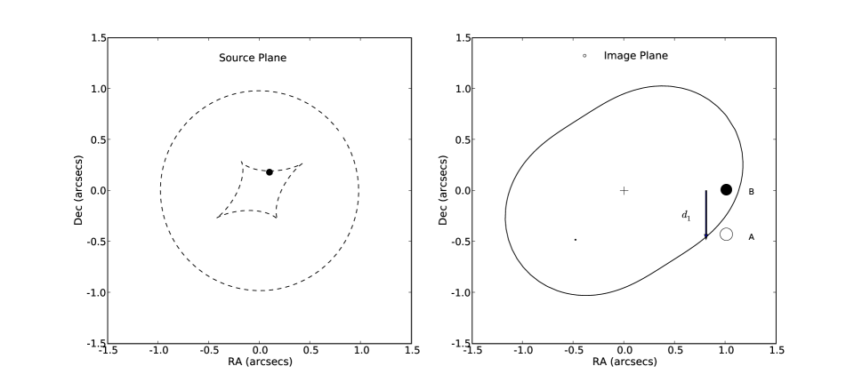
Figure 1.— A typical fold lens. Left: Source plane with caustic curves. Right: Image plane with critical curves. Images with negative magnification (parity) are denoted with filled circles, while images with positive magnification (parity) are open circles. Throughout the paper (and in most papers on fold lenses) Image A is the positive parity fold image, and Image B is the negative parity fold image. Following KGP, $d_{1}$ is the distance separating A and B.

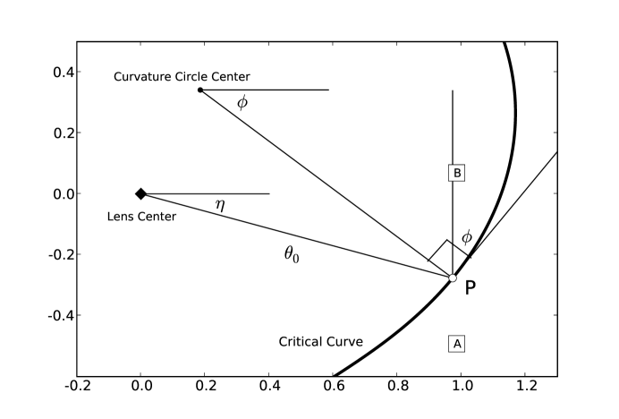
Figure 2.— The relative orientation of the fold images (A,B), the lens center, and the critical curve in our model. The point, ${\cal P}$, represents the position on the critical curve where the two images would meet if the source were moved closer to the caustic in the source plane. It is also the point around which all derivatives of the potential are defined.

Figure 3.— The measured and estimated flux anomaly parameter for a Singular Isothermal Sphere (SIS) lens with an external shear. This simulation, and those in subsequent figures, was produced using the lensmodel package. In each case, the lens has an Einstein radius of $\theta_{e}=1$, and in this model, there is an external shear of $\gamma^{e}=0.15$. As KGP have shown, we get dramatically different flux anomalies depending on where the source image lies along the caustic. Triangles represent sources near the edge of a caustic. We have uniformly placed 18 sources approximately 10% the characteristic scale from, and along the edge. The large flux ratios arise for sources nearer to the cusps. Unsurprisingly, those sources near cusps more strongly resemble “cusp lenses.” Since cusp lenses are expected to have a different flux relationship (in which the bright image equals the sum of two dimmer ones), it is unsurprising that the flux anomaly between two images can be rather large. Indeed, this is precisely the result found by KGP. In every case, the geometric reconstruction technique produces a very good fit ($\langle\delta A\rangle=0.02$, $\delta R\leq 0.01$). The 8 diamonds represent images placed radially inward from the center of the caustic to within 10% of the center of the source. Those with a small ($\delta A\simeq 0.1$) deviation from prediction are those closest to the center, and most closely resemble quad lenses, rather than true folds. The diagonal line is meant as a guide and has a slope of 1.

Figure 4.— The measured and estimated flux anomaly parameter for a Point Source (PS) lens with an external shear. In each case, the lens has an Einstein radius of $\theta_{e}=1$, and various systems were modeled with an external shear of $\gamma^{e}=0.2$ and $0.3$. Since most of the variation in flux anomaly arises for variations along the edge of the caustic, we use a slightly different set of symbols in this figure and subsequently than in the previous one. Triangles represent sources near the edge of a caustic, while squares represent sources closer to cusps. In both cases, there is a small systematic error in the anomaly parameter of $\langle\delta A\rangle\simeq 0.08$. This corresponds to a typical error in the flux anomaly of $\delta R\simeq 0.04$.

Figure 5.— The measured and estimated flux anomaly parameter for a Singular Isothermal Ellipsoid (SIE) with an ellipticity of 0.5. The fiducial lens has an Einstein radius of $\theta_{e}=1$. As in the previous figures, triangles represent sources near the edge of a caustic, while squares represent sources closer to cusps. Cuspy folds seem well modeled, with $\langle\delta A\rangle=-0.02$. However, sources further from the cusps had a larger systematic error, with $\langle\delta A\rangle\simeq-0.09$. This one-sided offset is primarily due to a flaw in our assumptions. Throughout, we’ve assumed that the shear only contributes in second derivatives of the potential. In future work, we may relax this condition somewhat and allow for an intrinsic elliptical potential.

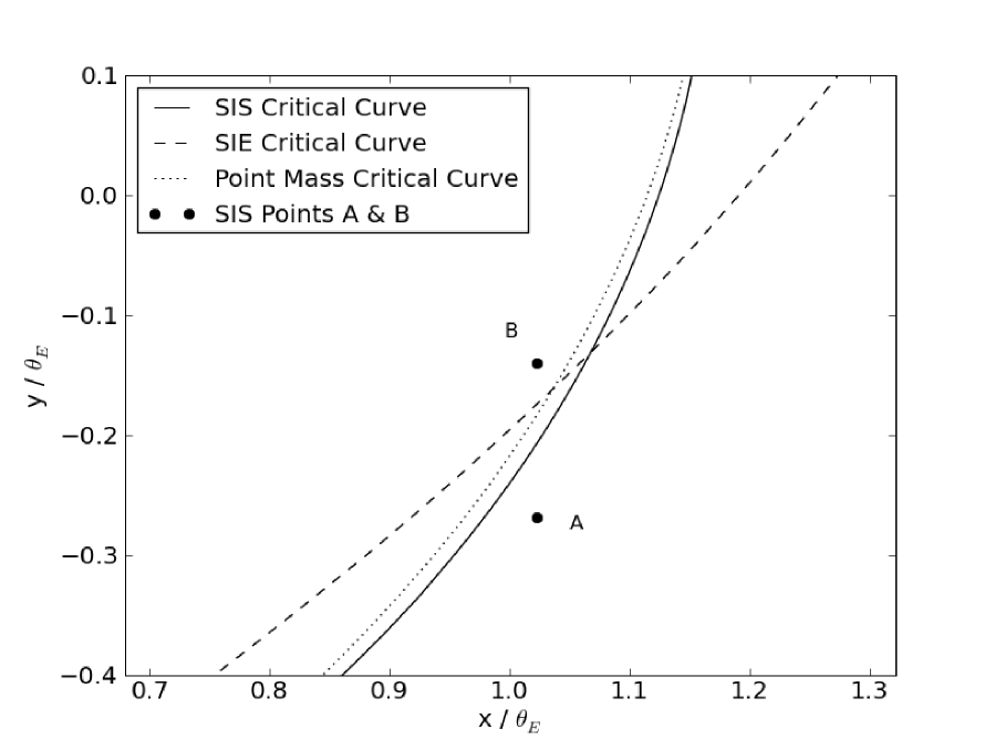
Figure 6.— The fold lens images for a simulated quad system with a Singular Isothermal Sphere ($\theta_{E}=1$) and an external shear with $\gamma_{e}=0.2$. Only the two fold images are shown in this plot, but the critical curves are fit to all four image positions, and the image centroid. Curves are fit for several models with external shear, as well as potentials with intrinsic ellipticity. The solid line critical curve represents a Singlular Isothermal Sphere with external shear, the dashed line represents a Singular Isothermal Ellipsoid and the dotted line represents a Point Source with external shear.

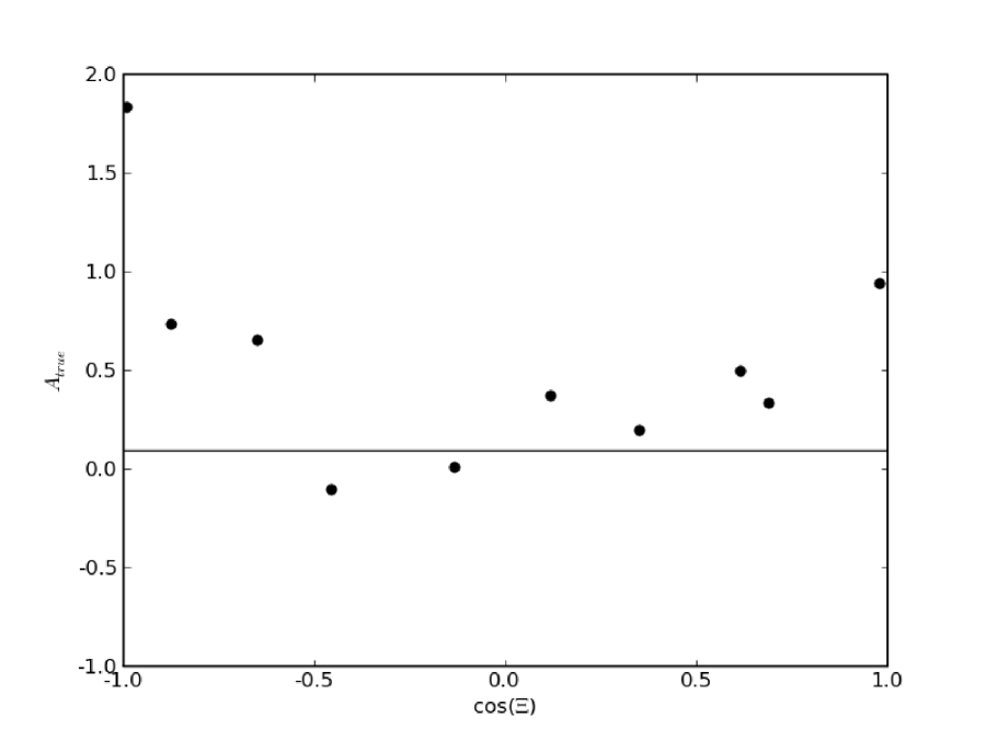
Figure 7.— As described in the text, the observed flux anomaly parameter for a variety of simulated fold lens systems. For each, a point mass with external shear was placed at the origin. In addition, a substructure with $\theta_{E}=0.2$ was placed a fixed separation (approximately equal to the image pair) such that the angle between the image separation and the secondary mass was $\Xi$.

Figure 8.— A comparison of our simulated Isothermal Sphere+external shear estimates of the fold relation (x-axis), with those estimated by KGP (diamonds with errorbars) from Monte Carlo simulation, and observed (triangles). This sample consists of the 10 quad systems in the radio and IR for which analysis was done by both groups. Note that our results have a very close correspondence ($\langle\Delta R\rangle\simeq 0.02$) with those done using Monte Carlo simulations, but make much simpler assumptions. Further, for about half the systems, the observed flux anomaly is very similar to those estimated by both groups.

References

- Angonin-Willaime et al. (1999) Angonin-Willaime, M., Vanderriest, C., Courbin, F., Burud, I., Magain, P., & Rigaut, F. 1999, A&A, 347, 434
- Anguita et al. (2008) Anguita, T., Faure, C., Yonehara, A., Wambsganss, J., Kneib, J.-P., Covone, G., & Alloin, D. 2008, A&A, 481, 615
- Bacon et al. (2006) Bacon, D. J., Goldberg, D. M., Rowe, B. T. P., & Taylor, A. N. 2006, MNRAS, 365, 414
- Biggs et al. (2004) Biggs, A. D., Browne, I. W. A., Jackson, N. J., York, T., Norbury, M. A., McKean, J. P., & Phillips, P. M. 2004, MNRAS, 350, 949
- Biggs et al. (2000) Biggs, A. D., Xanthopoulos, E., Browne, I. W. A., Koopmans, L. V. E., & Fassnacht, C. D. 2000, MNRAS, 318, 73
- Blandford & Narayan (1986) Blandford, R., & Narayan, R. 1986, ApJ, 310, 568
- Bradač et al. (2002) Bradač, M., Schneider, P., Steinmetz, M., Lombardi, M., King, L. J., & Porcas, R. 2002, A&A, 388, 373
- Chartas et al. (2004) Chartas, G., Eracleous, M., Agol, E., & Gallagher, S. C. 2004, ApJ, 606, 78
- Chiba et al. (2005) Chiba, M., Minezaki, T., Kashikawa, N., Kataza, H., & Inoue, K. T. 2005, ApJ, 627, 53
- Congdon & Keeton (2005) Congdon, A. B., & Keeton, C. R. 2005, MNRAS, 364, 1459
- Congdon et al. (2008) Congdon, A. B., Keeton, C. R., & Nordgren, C. E. 2008, MNRAS, 389, 398
- Dalal & Kochanek (2002) Dalal, N., & Kochanek, C. S. 2002, ApJ, 572, 25
- Dobler & Keeton (2006) Dobler, G., & Keeton, C. R. 2006, MNRAS, 365, 1243
- Evans & Witt (2003) Evans, N. W., & Witt, H. J. 2003, MNRAS, 345, 1351
- Fassnacht et al. (1999) Fassnacht, C. D., Pearson, T. J., Readhead, A. C. S., Browne, I. W. A., Koopmans, L. V. E., Myers, S. T., & Wilkinson, P. N. 1999, ApJ, 527, 498
- Fassnacht et al. (2002) Fassnacht, C. D., Xanthopoulos, E., Koopmans, L. V. E., & Rusin, D. 2002, ApJ, 581, 823
- Goldberg & Bacon (2005) Goldberg, D. M., & Bacon, D. J. 2005, ApJ, 619, 741
- Hewitt et al. (1992) Hewitt, J. N., Turner, E. L., Lawrence, C. R., Schneider, D. P., & Brody, J. P. 1992, AJ, 104, 968
- Holder & Schechter (2003) Holder, G. P., & Schechter, P. L. 2003, ApJ, 589, 688
- Impey et al. (1998) Impey, C. D., Falco, E. E., Kochanek, C. S., Lehár, J., McLeod, B. A., Rix, H., Peng, C. Y., & Keeton, C. R. 1998, ApJ, 509, 551
- Inada et al. (2003) Inada, N., et al. 2003, Nature, 426, 810
- Inada et al. (2005) —. 2005, PASJ, 57, L7
- Jackson et al. (2000) Jackson, N., Xanthopoulos, E., & Browne, I. W. A. 2000, MNRAS, 311, 389
- Jackson et al. (1998) Jackson, N., et al. 1998, MNRAS, 296, 483
- Katz & Hewitt (1993) Katz, C. A., & Hewitt, J. N. 1993, ApJ, 409, L9
- Katz et al. (1997) Katz, C. A., Moore, C. B., & Hewitt, J. N. 1997, ApJ, 475, 512
- Keeton (2001) Keeton, C. R. 2001, ArXiv Astrophysics e-prints
- Keeton (2003) —. 2003, ApJ, 584, 664
- Keeton et al. (2006) Keeton, C. R., Burles, S., Schechter, P. L., & Wambsganss, J. 2006, ApJ, 639, 1
- Keeton et al. (2003) Keeton, C. R., Gaudi, B. S., & Petters, A. O. 2003, ApJ, 598, 138
- Keeton et al. (2005) —. 2005, ApJ, 635, 35
- Keeton et al. (1997) Keeton, C. R., Kochanek, C. S., & Seljak, U. 1997, ApJ, 482, 604
- King et al. (1997) King, L. J., Browne, I. W. A., Muxlow, T. W. B., Narasimha, D., Patnaik, A. R., Porcas, R. W., & Wilkinson, P. N. 1997, MNRAS, 289, 450
- King et al. (1998) King, L. J., et al. 1998, MNRAS, 295, L41+
- Kochanek et al. (2004) Kochanek, C. S., Schneider, P., & Wambsganss, J. 2004, astro-ph/0407232
- Koopmans & de Bruyn (2000) Koopmans, L. V. E., & de Bruyn, A. G. 2000, A&A, 358, 793
- Koopmans et al. (2003) Koopmans, L. V. E., et al. 2003, ApJ, 595, 712
- Lawrence et al. (1995) Lawrence, C. R., Elston, R., Januzzi, B. T., & Turner, E. L. 1995, AJ, 110, 2570
- Mao & Schneider (1998) Mao, S., & Schneider, P. 1998, MNRAS, 295, 587
- Marlow et al. (1999a) Marlow, D. R., Browne, I. W. A., Jackson, N., & Wilkinson, P. N. 1999a, MNRAS, 305, 15
- Marlow et al. (1999b) Marlow, D. R., et al. 1999b, AJ, 118, 654
- Metcalf & Madau (2001) Metcalf, R. B., & Madau, P. 2001, ApJ, 563, 9
- Miranda & Jetzer (2007) Miranda, M., & Jetzer, P. 2007, Ap&SS, 312, 203
- More et al. (2009) More, A., McKean, J. P., More, S., Porcas, R. W., Koopmans, L. V. E., & Garrett, M. A. 2009, MNRAS, 394, 174
- Morgan et al. (2006) Morgan, C. W., Kochanek, C. S., Morgan, N. D., & Falco, E. E. 2006, ApJ, 647, 874
- Muñoz et al. (2001) Muñoz, J. A., Kochanek, C. S., & Keeton, C. R. 2001, ApJ, 558, 657
- Myers et al. (1995) Myers, S. T., et al. 1995, ApJ, 447, L5+
- Nair (1998) Nair, S. 1998, MNRAS, 301, 315
- Oguri et al. (2008) Oguri, M., Inada, N., Blackburne, J. A., Shin, M., Kayo, I., Strauss, M. A., Schneider, D. P., & York, D. G. 2008, MNRAS, 391, 1973
- Petters et al. (2001) Petters, A. O., Levine, H., & Wambsganss, J. 2001, Singularity theory and gravitational lensing (Birkhauser)
- Phillips et al. (2000) Phillips, P. M., et al. 2000, MNRAS, 319, L7
- Pooley et al. (2007) Pooley, D., Blackburne, J. A., Rappaport, S., & Schechter, P. L. 2007, ApJ, 661, 19
- Pooley et al. (2006) Pooley, D., Blackburne, J. A., Rappaport, S., Schechter, P. L., & Fong, W.-f. 2006, ApJ, 648, 67
- Reimers et al. (2002) Reimers, D., Hagen, H.-J., Baade, R., Lopez, S., & Tytler, D. 2002, A&A, 382, L26
- Schechter & Wambsganss (2002) Schechter, P. L., & Wambsganss, J. 2002, ApJ, 580, 685
- Schneider et al. (1986) Schneider, D. P., Gunn, J. E., Turner, E. L., Lawrence, C. R., Hewitt, J. N., Schmidt, M., & Burke, B. F. 1986, AJ, 91, 991
- Schneider et al. (1985) Schneider, D. P., Lawrence, C. R., Schmidt, M., Gunn, J. E., Turner, E. L., Burke, B. F., & Dhawan, V. 1985, ApJ, 294, 66
- Schneider et al. (1992) Schneider, P., Ehlers, J., & Falco, E. E. 1992, Gravitational Lenses, ed. Schneider, P., Ehlers, J., & Falco, E. E.
- Snellen et al. (1995) Snellen, I. A. G., de Bruyn, A. G., Schilizzi, R. T., Miley, G. K., & Myers, S. T. 1995, ApJ, 447, L9+
- Sykes et al. (1998) Sykes, C. M., et al. 1998, MNRAS, 301, 310
- Williams et al. (2008) Williams, L. L. R., Foley, P., Farnsworth, D., & Belter, J. 2008, ApJ, 685, 725