Numerical simulations of imbalanced strong magnetohydrodynamic turbulence

Abstract

Magnetohydrodynamics (MHD) is invoked to address turbulent fluctuations in a variety of astrophysical systems. MHD turbulence in nature is often anisotropic and imbalanced, in that Alfvénic fluctuations moving in opposite directions along the background magnetic field carry unequal energies. This work formulates specific requirements for effective numerical simulations of strong imbalanced MHD turbulence with a guide field $\mathbf{B}_{0}$. High-resolution simulations are then performed and they suggest that the spectra of the counter-propagating Alfvén modes do not differ from the balanced case, while their amplitudes and the corresponding rates of energy cascades are significantly affected by the imbalance. It is further proposed that the stronger the imbalance the larger the magnetic Reynolds number that is required in numerical simulations in order to correctly reproduce the turbulence spectrum. This may explain current discrepancies among numerical simulations and observations of imbalanced MHD turbulence.

1. Introduction

Magnetohydrodynamic (MHD) turbulence plays a critical role in theoretical modeling of the spectra of velocity and magnetic fluctuations in the Solar Wind (e.g., Coleman, 1966, 1968; Belcher & Davis, 1971; Marsch, 1991; Goldstein et al., 1995) as well as electron density fluctuations in the interstellar medium (e.g., Armstrong et al., 1995; Lithwick & Goldreich, 2001). Following the pioneering works of Iroshnikov (1963) and Kraichnan (1965), and the introduction of the concept of critical balance by Goldreich & Sridhar (1995), progress in MHD turbulence was mostly due to phenomenological models, closure theories, and weak turbulence asymptotic models. In recent years, constantly increasing computing power has put within our reach the ability to simulate universal inertial range spectra of strong MHD turbulence (e.g., Cho & Vishniac, 2000; Maron & Goldreich, 2001; Haugen et al., 2003; Biskamp, 2003; Müller & Grappin, 2005; Mason et al., 2006, 2008; Mininni & Pouquet, 2007; Beresnyak & Lazarian, 2008; Perez & Boldyrev, 2008, 2009). These simulations have motivated new phenomenological models and have revived the vigorous interest in the fundamentals of MHD turbulence.

As an important result, simulations have shown that strong MHD turbulence is locally imbalanced, that is, it spontaneously develops correlated regions of positive and negative cross-helicity where the energy in Alfvén waves propagating along and against the magnetic field are not equal, irrespective of the total amount of cross-helicity in the system, see Perez & Boldyrev (2009); Boldyrev et al. (2009). In each of these regions both energy and cross helicity are subject to a nonlinear cascade from large to small scales, consequently having an effect in the overall energy spectrum.

Such an imbalance is clearly present in the solar wind, where velocity and magnetic fluctuations show high correlations of a preferred sign, that is, the normalized cross helicity $\sigma_{c}={\left\langle\mathbf{v}\cdot\mathbf{b}\right\rangle}/{E}={H_{c}}/{E}$ is predominantly close to unity. Here $E$ is the average total energy (kinetic plus magnetic), $H_{c}$ is the cross helicity and the brackets denote a suitable ensemble average. The preferred positive sign of $\sigma_{c}$ indicates that there is more energy in Alfvén waves propagating outwards from the Sun than propagating inwards.

Several phenomenological models have been proposed to address strong imbalanced MHD turbulence (Lithwick et al. (2007); Chandran (2008); Beresnyak & Lazarian (2008); Perez & Boldyrev (2009); Podesta & Bhattacharjee (2009)), some with support from numerical simulations and observations. However, these works have led to conflicting predictions. For instance, the theory by Lithwick et al. concludes that in imbalanced regions the Elsässer spectra have the same scalings $E^{+}(k_{\perp})\propto E^{-}(k_{\perp})\propto k_{\perp}^{-5/3}$. The theory by Chandran proposes that the spectra of $E^{+}(k_{\perp})$ and $E^{-}(k_{\perp})$ are different depending of the degree of imbalance. The theory by Beresnyak & Lazarian also suggests the different spectra for $E^{+}(k_{\perp})$ and $E^{-}(k_{\perp})$. Finally, the analysis by Perez & Boldyrev and Podesta & Bhattacharjee finds that the spectra of $E^{+}(k_{\perp})$ and $E^{-}(k_{\perp})$ have different amplitudes but the same scalings $E^{+}(k_{\perp})\propto E^{-}(k_{\perp})\propto k_{\perp}^{-3/2}$.

On the numerical side, anisotropy and imbalance significantly complicate simulations of MHD turbulence. In the presence of a strong guide field, the turbulent fluctuations become elongated in the direction of the field. This increases the variety of numerical settings that can be used to drive such turbulence and complicates comparison of numerical simulations carried out by different groups. For example, numerical settings can include weak or strong guide fields; different levels of imbalance; cubic or rectangular simulation boxes; short or long-time correlated large-scale forces; frozen large-scale modes; forcing that excites only $\mathbf{v}$, $\mathbf{b}$ or both; volume forcing or forcing at the boundaries of the domain; different resolutions along field-perpendicular and field-parallel directions, etc.

To understand how different numerical simulations can be compared to each other, one needs to understand the conditions that should be met to ensure that simulations reproduce the range of scales where turbulence is universal. For instance, one has to be sure that the forcing and the dissipation do not spoil the inertial interval. The first steps in this direction were made in (Mason et al., 2006; Perez & Boldyrev, 2008) for the balanced case. It was found that the inertial range scaling can be sensitive to the way in which the turbulence is forced, not because of a lack of universality, but because the inertial range has a limited extent.

In the present paper we formulate the conditions that need to be satisfied in order to correctly simulate strong imbalanced MHD turbulence. We then propose a universal numerical setting, based on the reduced MHD model, which allows one to find the spectra of both balanced and imbalanced MHD turbulence. We found that imbalance significantly reduces the inertial interval in numerical simulations. The numerical resolution required to produce a large inertial interval strongly increases with the amount of imbalance. An imbalance essentially stronger than $\gamma^{2}=(z^{+})^{2}/(z^{-})^{2}\sim 10$ cannot be accessed with currently available supercomputers, which significantly limits the applicability of present-day numerical simulations to practical cases.

2. Model equations

In the presence of a guide field ${\bf B_{0}}$ (say in the $z$ direction), the MHD equations describing the evolution of magnetic and velocity fluctuations, ${\bf b}(\mathbf{x},t)$ and ${\bf v}(\mathbf{x},t)$ can be written in terms of the so-called Elsässer variables, ${\bf z}^{\pm}={\bf v}\pm{\bf b}$:

$$\partial_{t}{\bf z}^{\pm}\mp({\bf V}_{A}\cdot\nabla){\bf z}^{\pm}+({\bf z}^{\mp}\cdot\nabla){\bf z}^{\pm}=-\nabla P+{\bf f},$$ (1)

where ${\bf V}_{A}={\bf B}_{0}/\sqrt{4\pi\rho}$ is the Alfvén velocity, $\rho$ is the fluid density, $P$ is the total pressure that is determined from the incompressibility condition, $\nabla\cdot{\bf z}^{\pm}=0$, ${\bf f}$ is large-scale forcing and we neglect small viscosity and resistivity. In the limit of weak fluctuations, the incompressible MHD system describes non-interacting Alfvén waves with dispersion relation $\omega^{\pm}(\mathbf{k})=\pm k_{\|}V_{A}$. These waves can have two types of polarizations, the shear-Alfvén one ($\mathbf{z}^{\pm}_{S}$) and the pseudo-Alfvén one ($\mathbf{z}^{\pm}_{P}$) given in Fourier space by $\mathbf{e}_{S}\equiv{\mathbf{e}_{\|}\times\mathbf{k}}/{k_{\perp}}$ and $\mathbf{e}_{P}\equiv{\mathbf{k}\times\mathbf{e}_{S}}/k$, where $\mathbf{e}_{\|}$ is a unit vector in $z$ direction. Strong MHD turbulence is dominated by fluctuations with $k_{\perp}\gg k_{\|}$. Goldreich & Sridhar (1995) argued that since for large $k_{\perp}$ the polarization of the pseudo-Alfvén fluctuations is almost parallel to the guide field, such fluctuations are coupled only to field-parallel gradients, which are small since $k_{\|}\ll k_{\perp}$. Therefore, the pseudo-Alfvén modes do not play a dynamically essential role in the turbulent cascade. We can remove the pseudo-Alfvén modes by setting $\mathbf{z}^{\pm}_{\|}=0$ in equations (1) to obtain

$$\partial_{t}{\tilde{\bf z}}^{\pm}\mp({\bf V}_{A}\cdot\nabla){\tilde{\bf z}}^{\pm}+({\tilde{\bf z}}^{\mp}\cdot\nabla){\tilde{\bf z}}^{\pm}=-\nabla_{\perp}P+\frac{1}{R}\nabla^{2}{\tilde{\bf z}}^{\pm},$$ (2)

where $R$ denotes the Reynolds numbers (discussed below). In this system, the fluctuating fields have only two vector components, ${\tilde{\bf z}}^{\pm}=\{{\tilde{z}}^{\pm}_{1},{\tilde{z}}^{\pm}_{2},0\}$, but depend on all three spatial coordinates. System (2) is equivalent to the Reduced MHD model, originally developed for tokamak plasmas by Kadomtsev & Pogutse (1974) and Strauss (1976).

3. Numerical strategy

Model (2) describing the nonlinear interactions of Shear-Alfvén modes is a valuable tool in theoretical and numerical studies of incompressible MHD turbulence. Based on this model, we now discuss the conditions that should be satisfied in order to correctly simulate strong MHD turbulence, both balanced and imbalanced.

3.1. Computation Domain

In the presence of a strong guide field the turbulence is anisotropic. According to Goldreich & Sridhar (1995), deep in the inertial range turbulence should become strong and the fluctuations should satisfy the critical balance condition $k_{\|}B_{0}\sim k_{\perp}b_{\lambda}$, where $k_{\|}\sim 1/l$ and $k_{\perp}\sim 1/\lambda$ are the field-parallel and field-perpendicular wave vectors associated to an anisotropic eddy of parallel size $l$ and perpendicular size $\lambda$, respectively. Let us define the nonlinear interaction strength parameter

$$\chi=(k_{\perp}b_{\lambda})/(k_{\|}B_{0});$$ (3)

the critical balance condition then implies $\chi\sim 1$.

Simulations of incompressible turbulence are generally based on the Fourier pseudo-spectral method. In order to allow for the inertial interval to develop, turbulence is driven at the lowest resolvable wave numbers, and the energy dissipates at large wave numbers determined by the Reynolds numbers. For simulations on a cubic periodic box of size $L$, the smallest wave-numbers along the field-parallel and field-perpendicular directions coincide, i.e., $k_{\perp}=k_{\|}=2\pi/L$. Therefore, driving at the low $k_{\|},k_{\perp}$ results in an isotropic forcing and the nonlinear strength parameter at the forcing scale becomes $\chi_{0}={k_{\perp}b_{\lambda}}/{k_{\|}B_{0}}\sim{b_{\lambda}}/{B_{0}}\ll 1$, which means that at least at the large scales, nonlinear interactions are weak. This would not be harmful if we had the resources to achieve arbitrarily high resolution, as the turbulence would proceed weakly until $\chi\sim 1$, and then would become strong. However, simulations generally produce a rather limited inertial range, so that the parameter $\chi$ can hardly reach unity in such a setup.

As pointed out by Maron & Goldreich (2001), and applied in recent simulations Mason et al. (2006); Perez & Boldyrev (2008), the best way to avoid this is to use an anisotropic domain such that at the forcing scale the parameter $\chi$ is already of order unity, that is, the excited large-scale modes are already anisotropic and satisfy the critical balance condition. To achieve this we choose an elongated box $L_{\perp}^{2}\times L_{\|}$, so that the lowest field-perpendicular and field-parallel wave-numbers are $k_{\perp}=2\pi/L_{\perp}$ and $k_{\|}=2\pi/L_{\|}$, respectively. In this case, forcing at the lowest $k_{\perp},k_{\|}$ leads to $\chi_{0}=L_{\|}b_{\lambda}/L_{\perp}B_{0},$ which is of order unity provided that

$${L_{\perp}}/{L_{\|}}\sim{b_{\lambda}}/{B_{0}}.$$ (4)

In this way, the turbulence is excited in a strong regime and the cascade proceeds down to smaller scales preserving the critical balance condition.

3.2. Numerical Resolution

At first sight, it appears that elongating the box along the $z$ direction to match the elongation of the eddies should not change the number of grid points required in this direction compared to the number of points in the $x$ and $y$ directions. Fortunately, the number of points in the $z$ direction can be reduced. This follows from the fact that the turbulent spectrum declines quite slowly, as a power-law, in the $k_{\perp}$ direction, while it drops sharply in the $k_{\|}$ direction for $k_{\|}>k_{\perp}^{\alpha}$, where $\alpha$ is a some positive power not exceeding 1 (Cho & Vishniac, 2000; Maron & Goldreich, 2001; Oughton et al., 2004; Perez & Boldyrev, 2008, 2009) . This qualitatively different spectral behavior in $k_{\|}$ and $k_{\perp}$ directions allows one to reduce the numerical resolution by a factor of 2 to 4 in the parallel direction, see Table 1. We checked that the restoration of the full resolution in the $z$ direction does not change the results, while significantly increases the computing costs.

3.3. Periodic Boundary Conditions

The spectral method assumes periodic boundary conditions in all spatial directions. The periodic boundary conditions in the z-direction may cause questions of whether the Alfvén modes counter-propagating along a given magnetic field line will always interact only among themselves. The answer is no, since periodicity of the fluctuations does not imply periodicity of the magnetic field lines. Magnetic field lines are not periodic, and each given eddy interacts with many independent counter-propagating eddies. One can check numerically, that reducing the parallel box size $L_{\|}$ below (4) somewhat spoils the spectrum at low wave numbers, e.g., as seen in forced simulations of (Müller & Grappin, 2005), while increasing it beyond (4) does not change the results, but increases the computational cost [Mason & Cattaneo, unpublished].

3.4. Reynolds numbers

Probably the most significant limitation is imposed by the consideration of imbalanced turbulence. Indeed, in the imbalanced case, $\gamma=z^{+}/z^{-}>1$, the formal Reynolds numbers corresponding to $\mathbf{z}^{+}$ and $\mathbf{z}^{-}$ fields are essentially different. Therefore, the resolution requirements increase with the amount of imbalance in order to produce large inertial ranges. Assume that the number of grid points in a field-perpendicular direction scales with the Reynolds number as $N\sim Re^{\beta}$, where $\beta=2/3$ or $3/4$ depending on the spectral slope ($3/2$ or $5/3$). Then increasing the imbalance $\gamma$ by, say, a factor of 3 will require increasing the resolution by approximately a factor of 2. Noting that resolution of at least 1024 is required to simulate the imbalance $\gamma\sim 2$ (see below), we conclude that significantly stronger imbalance is not achievable with present day computing power.

3.5. Random Forcing

In this section we discuss the important aspects to be considered when choosing a particular forcing. We assume a random force ${\tilde{\bf f}}$ that has no component along $z$, it is solenoidal in the $x-y$ plane and its Fourier coefficients outside the range $1\leq k_{\perp}\leq 2,\quad(2\pi/L_{\|})\leq k_{\|}\leq(2\pi/L_{\|})n_{z}$ are zero, where $n_{z}$ determines the width of the force spectrum in $k_{\|}$, and $L_{\perp}=2\pi$. The Fourier coefficients inside that range are Gaussian random numbers with amplitude chosen so that the resulting rms velocity fluctuations are of order unity. The individual random values are refreshed independently at time intervals $\tau$. The parameter $n_{z}$ controls the degree to which the critical balance condition is satisfied at the forcing scale. Note that we do not drive the $k_{\|}=0$ mode but allow it to be generated by nonlinear interactions.

In contrast with incompressible hydrodynamic system, an incompressible MHD system can support Alfvén waves. When the system is driven by a time dependent forcing, the most effectively driven modes are those resonating with the frequencies present in the forcing. Therefore, the spatial spectra of the large-scale velocity and magnetic fluctuations are not generally the same as the spatial spectrum of the force. Rather, they essentially depend on the both spatial and temporal spectra of the random forcing. Ultimately, it is the spectrum of the large-scale fluctuations, not the driving force, that should be controlled in numerical simulations.

In the following we perform simulations with a short-time-correlated random forcing that drives the turbulence close to the critical balance condition at the large scales. The short correlation time $\tau$ ensures a broadband frequency spectrum for the forcing, which allows high frequency Alfvén waves to be excited, so that one can control the width of the field-parallel spatial spectrum of the fluctuations by choosing the number of driven field-parallel modes, $n_{z}$. A sort-time correlated Gaussian random force has another important advantage. It allows one to control the rates at which the energies of $z^{+}$ and $z^{-}$ modes are injected.

Run	Resolution	$Re$	$\nu=\eta$	$L_{\|}/L_{\perp}$	$\sigma_{c}$
A1	$512^{2}\times 256$	2400	$4.2\times 10^{-4}$	5	0
A2	$1024^{2}\times 256$	6000	$1.7\times 10^{-4}$	5	0
B1	$256^{3}$	900	$1.1\times 10^{-3}$	10	0.6
B2	$512^{2}\times 256$	2200	$4.6\times 10^{-4}$	10	0.6
B3	$1024^{2}\times 256$	5600	$1.8\times 10^{-4}$	10	0.6

Table 1Summary of simulations of strong balanced turbulence (A1, A2) and strong imbalanced turbulence (B1, B2, B3).

4. Numerical results

Table 1 summarizes five representative simulations that incorporate all the aspects discussed in section 3. The simulations produce consistent and physically meaningful results for a range of Reynolds numbers and degrees of imbalance. Runs A are carried out for balanced turbulence, that is, $\sigma_{c}=0$. In runs B, cross helicity is injected at the forcing scale in such a way that $\sigma_{c}$ reaches a steady state of $\sim 0.6$. We use a short time-correlated forcing, compared to the Alfvén time of the excited modes, so that the energy injection rates for both $\mathbf{z}^{+}$ and $\mathbf{z}^{-}$ only depend on the variance of the imposed forcing, which is controlled in our simulations. In the imbalanced case, field-parallel box size is optimized to reach the critical balance at the large scales. Except for the Reynolds numbers, simulations B1, B2, and B3 have the exact same parameters including the energy injection rates, $\epsilon^{+}$ and $\epsilon^{-}$.

Since the background magnetic field must be strong, we choose $B_{0}=5$ in the $v_{rms}$ units, cf the discussion in (Mason et al., 2006). Time is normalized to the large scale eddy turnover time $\tau_{0}=L_{\perp}/2\pi v_{rms}$, where $L_{\perp}$ is the field-perpendicular box size. The Reynolds number is defined as $Re=v_{rms}(L_{\perp}/2\pi)/\nu$ and we have chosen the same value for the magnetic Reynolds number, $Rm={b}_{rms}(L_{\perp}/2\pi)/\eta$, denoting both by $R$ in (2). In each run, the average is performed over about 100 large-scale-eddy turnover times. The results are presented in Fig. (1).

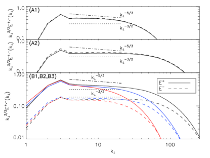
Figure 1.— Spectra of the Elsässer fields in numerical simulations of MHD turbulence. Top two frames: balanced turbulence (runs A1, A2); bottom frame: imbalanced turbulence (runs B1-B3).

5. Discussion

The advantage of our optimized setup (reduced MHD, elongated box, reduced resolution in z-direction) can be seen already in simulations of balanced turbulence, top frames in Fig. (1), runs A1 and A2. The energy spectra approach $E^{\pm}(k_{\perp})\propto k_{\perp}^{-3/2}$ in good agreement with earlier numerical findings (e.g., Maron & Goldreich, 2001; Haugen et al., 2003; Müller & Grappin, 2005; Mason et al., 2006), while our simulations require considerably less computational cost and produce slightly larger inertial intervals. Our most significant results are obtained for the imbalanced case. The bottom frame of Fig. 1 shows the spectra for three different Reynolds numbers (runs B1 to B3). It is observed that the spectra $E^{\pm}$ are pinned at the dissipation scales, which supports the phenomenological predictions by Grappin et al. (1983); Galtier et al. (2000); Lithwick & Goldreich (2003); Chandran (2008). We also find that the large-scale parts of the both spectra are practically insensitive to the Reynolds numbers. These two important properties imply that as the Re numbers are further increased, the $E^{\pm}$ spectra must become progressively more parallel in the inertial interval. This is indeed seen in our numerical simulations (B1-B3). Moreover, our numerical simulations indicate that both spectra approach the universal scaling of strong MHD turbulence $E^{\pm}(k_{\perp})\propto k_{\perp}^{-3/2}$, while they have essentially different amplitudes and correspond to essentially different energy fluxes.

The proposed numerical setup and the results of our simulations can serve as an important tool for resolving currently existing controversies regarding the spectra of imbalanced MHD turbulence. In particular, our results are consistent with the theories and observations predicting same scaling $-3/2$ for both Elsässer fields (Perez & Boldyrev, 2009; Podesta & Bhattacharjee, 2009). They are also broadly consistent with the theory by Lithwick et al. (2007), predicting the same scaling $-5/3$ for both fields. The major difference between the two phenomenologies is in the phenomenon of dynamic alignment that is taken into account in the former models and is not considered in the latter one. Our numerical findings are less consistent with the models predicting different scalings for the Elsässer fields $E^{\pm}$, (e.g., Chandran, 2008; Beresnyak & Lazarian, 2008). It would be interesting to understand what assumptions of these models disagree with the numerics. Finally, our analysis may explain somewhat puzzling numerical findings by Beresnyak & Lazarian (2009), who report different spectra for the $E^{\pm}$ Elsässer fields, and the intersection of the spectra rather than pinning at the dissipation scale. According to our results, the explanation might lie in the fact that in these simulations the imbalance was extremely high, up to $\gamma^{2}=(z^{+})^{2}/(z^{-})^{2}\sim 1000$, and, therefore, the universal regime of imbalanced MHD turbulence was not reached, see our analysis in Sec. 3.4.

This work was supported by the U.S. DOE grants No. DE-FG02-07ER54932 and DE-SC0001794, and by the NSF Center for Magnetic Self-Organization in Laboratory and Astrophysical Plasmas at the University of Wisconsin-Madison. High Performance Computing resources were provided by the Texas Advanced Computing Center (TACC) at the University of Texas at Austin under the NSF-Teragrid Project TG-PHY080013N.

References

- Armstrong et al. (1995) Armstrong, J. W., Rickett, B. J., & Spangler, S. R. 1995, ApJ, 443, 209
- Belcher & Davis (1971) Belcher, J. W. & Davis, Jr., L. 1971, J. Geophys. Res., 76, 3534
- Beresnyak & Lazarian (2008) Beresnyak, A. & Lazarian, A. 2008, ApJ, 682, 1070
- Beresnyak & Lazarian (2009) —. 2009, ApJ, 702, 460
- Biskamp (2003) Biskamp, D. 2003, Magnetohydrodynamic Turbulence, ed. D. Biskamp
- Boldyrev et al. (2009) Boldyrev, S., Mason, J., & Cattaneo, F. 2009, ApJ, 699, L39
- Chandran (2008) Chandran, B. D. G. 2008, ApJ, 685, 646
- Cho & Vishniac (2000) Cho, J. & Vishniac, E. T. 2000, ApJ, 539, 273
- Coleman (1966) Coleman, P. J. 1966, PRL, 17, 207
- Coleman (1968) Coleman, Jr., P. J. 1968, ApJ, 153, 371
- Galtier et al. (2000) Galtier, S., Nazarenko, S. V., Newell, A. C., & Pouquet, A. 2000, Journal of Plasma Physics, 63, 447
- Goldreich & Sridhar (1995) Goldreich, P. & Sridhar, S. 1995, ApJ, 438, 763
- Goldstein et al. (1995) Goldstein, M. L., Roberts, D. A., & Matthaeus, W. H. 1995, ARA&A, 33, 283
- Grappin et al. (1983) Grappin, R., Leorat, J., & Pouquet, A. 1983, A&A, 126, 51
- Haugen et al. (2003) Haugen, N. E. L., Brandenburg, A., & Dobler, W. 2003, ApJ, 597, L141
- Iroshnikov (1963) Iroshnikov, P. S. 1963, AZh, 40, 742
- Kadomtsev & Pogutse (1974) Kadomtsev, B. B. & Pogutse, O. P. 1974, JETP, 38, 283
- Kraichnan (1965) Kraichnan, R. H. 1965, Physics of Fluids, 8, 1385
- Lithwick & Goldreich (2001) Lithwick, Y. & Goldreich, P. 2001, ApJ, 562, 279
- Lithwick & Goldreich (2003) —. 2003, ApJ, 582, 1220
- Lithwick et al. (2007) Lithwick, Y., Goldreich, P., & Sridhar, S. 2007, ApJ, 655, 269
- Maron & Goldreich (2001) Maron, J. & Goldreich, P. 2001, ApJ, 554, 1175
- Marsch (1991) Marsch, E. MHD turbulence in the solar wind., 159–241
- Mason et al. (2006) Mason, J., Cattaneo, F., & Boldyrev, S. 2006, PRL, 97, 255002
- Mason et al. (2008) —. 2008, Phys. Rev. E, 77, 036403
- Mininni & Pouquet (2007) Mininni, P. D. & Pouquet, A. 2007, PRL, 99, 254502
- Müller & Grappin (2005) Müller, W.-C. & Grappin, R. 2005, PRL, 95, 114502
- Oughton et al. (2004) Oughton, S., Dmitruk, P., & Matthaeus, W. H. 2004, Physics of Plasmas, 11, 2214
- Perez & Boldyrev (2008) Perez, J. C. & Boldyrev, S. 2008, ApJ, 672, L61
- Perez & Boldyrev (2009) —. 2009, PRL, 102, 025003
- Podesta & Bhattacharjee (2009) Podesta, J. J. & Bhattacharjee, A. 2009, ArXiv e-prints
- Strauss (1976) Strauss, H. R. 1976, Physics of Fluids, 19, 134