Restrictions on the injection energy of positrons annihilating near the Galactic center

Abstract

The origin and properties of the source of positrons annihilating in the Galactic Center is still a mystery. One of the criterion, which may discriminate between different mechanisms of positron production there, is the positron energy injection. Beacom and Yüksel (2006) suggested a method to estimate this energy from the ratio of the 511 keV line to the MeV in-flight annihilation fluxes. From the COMPTEL data they derived that the maximum injection energy of positron should be about several MeV that cut down significantly a class of models of positron origin in the GC assuming that positrons lose their energy by Coulomb collisions only. However, observations show that the strength of magnetic field in the GC is much higher than in other parts of the Galaxy, and it may range there from 100 $\mu$G to several mG. In these conditions, synchrotron losses of positrons are significant that extends the range of acceptable values of positron injection energy. We show that if positrons injection in the GC is non-stationary and magnetic field is higher than 0.4 mG both radio and gamma-ray restrictions permit their energy to be higher than several GeV.

1 Introduction

One of the interesting and still unsolved problems is the origin of 511 keV annihilation emission from the Galactic Bulge. It is observed as an extended diffuse emission from $5^{\circ}-8^{\circ}$ radius region with the flux $\sim 8\times 10^{-4}$ ph cm^-2s^-1 that requires the rate of positron production there $\sim 10^{43}$ s^-1 (Knödlseder et al., 2005; Churazov et al., 2005; Jean et al., 2006). These observations showed that the energy of annihilating positrons was about 1 eV. On the other hand, all potential sources of positrons in the Galaxy like SN stars (Knödlseder et al., 2005), massive stars generating the radioactive ²⁶Al (Prantzos, 2006), secondary positrons from p-p collisions (Cheng et al., 2007), lepton jets of AGNs (Totani, 2006), dark matter annihilation (Boehm et al, 2004; Sizun et al., 2006), microquasars and X-ray binaries (Weidenspointner et al., 2008; Bandyopadhyay et al., 2007) etc. generate positrons with energies $\ga 1$ MeV. This means that positrons should effectively lose their energy before annihilation and thus generate emission in other than 511 keV energy ranges. Therefore, the injection energy of positrons is an essential parameter for modeling annihilation processes, and it can be in principle discriminated from observations.

High energy positrons annihilate ”in-flight”, thus producing continuum emission in the range $E>511$ keV. A prominent 511 keV line emission is generated by these positrons when their energy is decreased to the thermal one due to energy losses. Therefore, one can expect that the continuum and line emission are proportional to each other.

For the lifetime of in-flight annihilation, $\tau_{if}$, and the average cooling time $\tau_{cl}$ of high energy positrons, one can estimate the expected flux of in-flight annihilation, $F_{\mbox{1-30 MeV}}$ from the observed 511 keV line emission, $I_{line}$, as

$$F_{1-30~{}\mbox{MeV}}\sim\frac{\tau_{cl}}{\tau_{if}}I_{line}~{}~{}~{}~{}\mbox{if $\tau_{if}\gg\tau_{cl}$}$$ (1)

where

$$\tau_{if}=\left[n\sigma_{if}(E)v(E)\right]^{-1}$$ (2)

and

$$\tau_{cl}=\int\limits_{E_{inj}}^{E_{th}}\frac{dE}{\left(dE/dt\right)_{cl}}$$ (3)

Here $n$ is the plasma density, and $E_{inj}$, $E_{th}$ and $v(E)$ are the injection energy of positrons, the energy of thermal plasma, and the positron velocity, respectively, $\sigma_{if}$ is the cross-section of in-flight annihilation. The function $(dE/dt)_{cl}$ is the rate of energy losses defined as sum of Coulomb, synchrotron, inverse Compton, bremsstrahlung etc. losses:

$$\left(dE/dt\right)_{cl}=\left(dE/dt\right)_{coul}+\left(dE/dt\right)_{syn}+$$ (4)

$$+\left(dE/dt\right)_{IC}+\left(dE/dt\right)_{br}+...$$

If cooling of the positrons is only due to the Coulomb losses, then $\tau_{if}$ and $\tau_{cl}$ are proportional to $n^{-1}$, and the relation (1) is independent of the medium density. So, this ratio of the continuum in-flight and the annihilation emission is universal and can be applied even to a medium with an unknown density. Beacom and Yüksel (2006) assumed that positrons in the Galactic center (GC) loose their energy by Coulomb interactions only, and they suggested to use this ratio for the analysis of the annihilating positron origin in the GC. In the above-mentioned models the injection energy of positrons is expected in the range from several to hundreds MeV. Therefore, the in-flight gamma-ray emission is also expected in this energy range.

The MeV flux from the central part of the Galaxy was observed by COMPTEL (see, Strong et al., 1998). The origin of this emission is still unclear since the known processes of gamma-ray production (like inverse Compton, bremsstrahlung etc.) are unable to generate the observed flux (Strong et al., 2005; Porter et al., 2008). Cheng et al. (2007) assumed that this excess in the GC direction might be due to the in-flight annihilation of fast positrons. However, it is observed not only in the direction of the GC. The excess is almost constant along the Galactic disk (Strong et al., 1998) where the intensity of annihilation emission is lower than in the Galactic centre. This makes problematic the in-flight interpretation of this excess in the disk since the ratio 511 keV flux/in-flight continuum is constant. If the in-flight flux is responsible for the MeV excess in a relatively narrow central region ($\la 5^{\circ}$), absolutely the same excess in other parts of the disk remains unexplained (see Sizun et al., 2006; Chernyshov et al., 2008).

Therefore, in Beacom and Yüksel (2006) and latter in Sizun et al. (2006) a more firm constraint on the in-flight gamma-ray flux from the Galactic center was suggested. According to their criterion the in-flight flux should not exceed several statistical errors of the COMPTEL measurements. That gives an upper limit for the injection energy about several MeV. Then models assuming higher injection energy should undoubtedly be rejected.

Below we show that under some conditions the injection energy may be higher than 10 MeV in contrast to conclusions made in papers mentioned above, and, thus, there is a room for models assuming injection of high energy positrons.

Thus, Cheng et al. (2006, 2007) assumed that these positrons are secondary and generated by collisions of relativistic protons injected from black hole jets. The theoretical analysis of Istomin & Sol (2009) confirmed the hadronic origin of jets and showed that protons were accelerated there by the stochastic and the centrifugal acceleration up to energies $E_{p}\simeq 10^{20}$ eV that might offer an explanation to the recent results of the Pierre Auger collaboration (Abraham et al., 2007). If such or similar mechanism produces indeed enough relativistic protons with Lorentz factor $\gamma\ga 2$ in the vicinity of the central black hole then we do expect there an effective production of secondary positrons with energies above 30 MeV, just as assumed in Cheng et al. (2006, 2007).

Processes of $p-p$ collisions produce also a flux of gamma-rays in the range above 100 MeV by decay of $\pi^{\circ}$-meson, and below this energy by, so-called, internal bremsstrahlung radiation of secondary electrons (see for detail Hayakawa, 1964). A flux of gamma-rays in the 1 to 30 MeV range from internal bremsstrahlung may be higher than the mentioned in-flight flux. Thus, Beacom et al. (2005) showed that the internal bremsstrahlung flux is very significant, if positrons in the GC are generated by dark matter annihilation. However, in the dark matter model positron production in the GC is stationary. On the other hand, from the restrictions derived from EGRET data it follows that the positron production in the GC should be strongly non-stationary, if these positrons are generated by $p-p$ collisions (Cheng et al., 2006, 2007). The flux of gamma-rays from $p-p$ collisions is significant during a very short period after a star accretion onto the black hole. At present this flux has decreased in several orders of magnitude from its initial value and, therefore, is unseen.

Below in section 3 we shall show that the condition of non-stationarity is also required to fit radio observations.

2 Medium properties in the vicinity of the Galactic center

As follows from observations, the central 200 pc region of the Galaxy is strongly nonuniform. The inner bulge (200-300 pc) contains $(7-9)\times 10^{7}~{}M_{\odot}$ of hydrogen gas. In spite of relatively small radius this region contains about 10% of the Galaxy’s molecular mass. Most of the molecular gas is contained in very compact clouds of mass $10^{4}-10^{6}M_{\odot}$, average densities $\geq 10^{4}$cm^-3.

However, this molecular gas occupies a rather small part of the central region, most of which is filled with a very hot gas. ASCA Koyama et al. (1996) measured the X-ray spectrum in the inner 150 pc region which exhibited a number of emission lines from highly ionized elements which are characteristics for a $8-10$ keV plasma with the density 0.4 cm^-3. Later on Chandra observations of Muno et al. (2004) showed an intensive X-ray emission at the energy $E_{x}\sim 8$ keV from the inner 20 pc of the Galaxy. The plasma density was estimated in limits $0.1-0.2$ cm^-3. Recent SUZAKU measurements of the 6.9/6.7 keV iron line ratio (Koyama et al., 2007) was naturally explained by a thermal emission of 6.5 keV-temperature plasma.

One should note that there is no consensus on the magnetic field strength in the GC. Estimations ranges from about or smaller than hundred $\mu$G (see Spergel and Blitz, 1992; LaRosa et al., 2005; Higdon et al, 2009), up to several mG (Plante, Lo and Crutcher 1995; Yusef-Zadeh et al. 1999, see in this respect the review of Ferriere 2009). Radio observations of the central regions show that the structure of strong magnetic fields is nonuniform and it concentrates in filaments which extends up to 200 pc from the GC. The region containing mG magnetic field is estimated by the angular size $1.5\degr\times 0.5\degr$ (see e.g. Morris and Serabyn, 1996; Yusef-Zadeh, Hewitt and Cotton, 2004; Morris, 2006).

In these magnetic fields synchrotron losses are essential even for positrons with energies 3-30 MeV. One can see from Fig. 1 that if the magnetic field strength is as high as 3 mG, the cooling time of 1 GeV positrons is the same as that of positrons with energies about 1 MeV experiencing only Coulomb losses.

Structure of the magnetic field and the way electrons and positrons interact with it is also unknown. In our model we assumed that positrons interact with magnetic field structures violently thus allowing us to average the magnetic field over central 100 pc radius. However if the interaction is weak and can be neglected the original constraints deduced by Beacom and Yüksel (2006) prevail.

We shall show that the injection energy of positrons can be much higher than 1 MeV because of synchrotron losses in the Galactic center that extends significantly the class of models explaining the origin of annihilation emission from the bulge.

If it is not specified we accepted below that the central 100 pc radius region is filled with strong magnetic field and the gas density in the central region ($r\la 500$ pc) is $\ga 0.2$ cm^-3. The rate of ionization losses depends on the medium ionization degree. Therefore, we consider two cases of neutral and fully ionized medium.

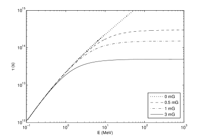
Figure 1: Characteristic cooling times of positrons for different values of magnetic field strength.

3 Effects of Strong Magnetic Fields in the GC

If positrons propagate through the region of strong magnetic fields in the GC, they effectively lose their energy and emit radiation in the radio range of frequencies. Thus, for $H=3$ mG positrons with energies 10-100 MeV generate emission in the range

$$\nu_{0}=0.29\frac{3eH}{4\pi mc}\left(\frac{E}{mc^{2}}\right)^{2}\sim 1-100~{}\mbox{MHz}$$ (5)

For the magnetic field of 3 mG the rate of synchrotron losses of relativistic electrons and positrons is higher than for any other process of losses. Therefore, an intensive synchrotron emission is expected from this region.

Observations of the GC gave the following values of radio flux from there (see, e.g., Mezger et al., 1996; LaRosa et al., 2005). This flux is about 10 kJy in the frequency range 300 - 700 MHz for the central region $3^{\circ}\times 2^{\circ}$. For the region $1.5^{\circ}\times 0.5^{\circ}$ this flux is almost one order of the magnitude smaller at the frequency 330 MHz, i.e. $\sim 1$ kJy.

On the other hand, simple estimations of synchrotron emission shows that if electrons and positrons are injected with energies about 100 MeV, then the radio flux from the GC is much higher than 1 kJy.

Below we demonstrate this point from very simple estimates of the radio emission from the GC. In the stationary state the total spectrum of positron in the GC injected at the energy $E_{0}$ with the rate $Q$ is

$$N(E)\simeq\frac{Q}{|dE/dt|}\theta(E_{0}-E)$$ (6)

where the rate of synchrotron losses is

$$\frac{dE}{dt}=-\frac{2}{3}\frac{e^{4}H^{2}}{c^{3}m^{2}}\left(\frac{E}{mc^{2}}\right)^{2}=-\beta E^{2}$$ (7)

Here and below $N(E)$ is the density of electrons and positrons with energy E. The radio flux from the GC at Earth can be calculated from the integral

$$\Phi_{\nu}=\frac{1}{4\pi d^{2}}\int\limits_{E}N(E)P(\nu,E)dE$$ (8)

where $P(\nu,E)$ is the emissivity of a single positron with the energy $E$, and $d=8$ kpc is the distance between Earth and the GC. To get an estimation we use the approximation for the function $P$ from Berezinskii et al. (1990)

$$P(\nu,E)\simeq\frac{dE}{dt}\delta\left(\nu-\nu_{0}(E)\right)$$ (9)

Then we have the the radio flux at the frequency $\nu$

$$\Phi_{\nu}=\frac{Q}{8\pi d^{2}}\frac{mc^{2}}{\nu}\sqrt{{\nu}/{\bar{\nu}}}$$ (10)

where $\bar{\nu}=\sqrt{0.29\cdot 3eH/4\pi mc}$. For the production rate of secondary electrons $Q=2\cdot 10^{43}$s^-1, this equation gives a flux at Earth about $10^{9}$ Jy at the frequency $\nu\sim 100$ MHz that is several order of magnitude higher than observed. This means that either the magnetic field strength and the injection energy of positrons should be smaller than those used in this estimation or the situation is strongly non-stationary.

For estimations of the non-stationary case we use the source function in the form

$$Q(E,t)=N_{0}\delta(t)\delta(E-E_{0})$$ (11)

where $N_{0}$ is the total number of injected positrons. Then the distribution function of positrons is (see section 5)

$$N(E,t)=N_{0}\delta\left(E-\frac{E_{0}}{\beta E_{0}t+1}\right)$$ (12)

where $\beta$ is the coefficient in Eq. (7), and the radio flux has the form

$$\Phi_{\nu}\sim\frac{N_{0}}{\nu{\left(E=\frac{E_{0}}{\beta E_{0}t+1}\right)}}\left.\frac{dE}{dt}\right|_{E=\frac{E_{0}}{\beta E_{0}t+1}}$$ (13)

As one can see that the current energy of electrons is independent of their injection energy $E_{0}$ and equals $E\simeq 1/\beta t$ for long enough $t$.

From Eq.(13) it follows that the radio flux just after the injection of positrons equals $\sim 3\cdot 10^{7}$ Jy for the $N_{0}\simeq 2\cdot 10^{55}$ in each capture events that is necessary to produce the observed annihilation flux from the GC. However, for the time $t\simeq 10^{5}$ years (the average period between str captures) the peak of intensity shifts from the frequency 100 MHz to several MHz where this radio flux cannot be observed because of absorption in the interstellar gas, and just this effect is a key point of our analysis presented below.

As an example we show in Fig. 2 the spectrum radio emission from the GC region produced by secondary electrons and positrons at the time $10^{5}$ yr after the capture. The magnetic field strength in the GC is 2 and 3 mG. As one can see for long time after the capture the peak of emission shifts from the frequency of hundreds MHz to several MHz, and the intensity of radio emission is negligible at 330 MHz. For calculations of radio emission we used the accurate equation (from e.g. Berezinskii et al., 1990),

$$\Phi(\nu,t)_{s}=\frac{1}{4\pi d^{2}}\frac{\sqrt{3}e^{3}H}{mc^{2}}\int\limits_{0}^{\infty}N(E,t)dE\frac{\nu}{\nu_{c}}\int\limits_{\nu/\nu_{c}}^{\infty}dzK_{5/3}(z)$$ (14)

where $N(E)$ is the total number of electrons and positrons with the energy $E$, $d=8$ kpc is the distance to the GC, and $K_{\alpha}(x)$ is the McDonald function.

In Fig. 3 we presented the limitations of positron injection energy $E_{0}$ derived from radio data for different values of the magnetic field strength and different times T passed from the last star capture. We considered two possible cases: the injection in the form of delta-function, Eq. (11), shown in the figure by solid lines and power-law injection spectrum (dashed line):

$$N_{0}(E)=N_{0}\delta(t)E^{-3}\theta(E-E_{0})~{}\mbox{.}$$ (15)

One can see that if the injection is non-stationary, then the injection energy of positrons can be extremely high in case of strong magnetic fields in the GC. Indeed for almost stationary situation when characteristic period between injections is small $T\leq 1\times 10^{4}$ yr the maximum allowed energy in case of $H\geq 1$ mG cannot exceed 30 MeV due to radio limitations. In case of power-law spectrum situation is even worse. However if period is long enough and magnetic field is strong the situation changes: for $T=1\times 10^{5}$ yr and $H=2$ mG the maximum energy is about 1 GeV and it can be even higher for longer periods and higher values of the magnetic field.

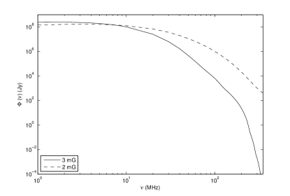
Figure 2: Radio flux at Earth produced by positrons from a single capture event at the time $10^{5}$ yr after the capture. The strength of magnetic field $H=3$ mG (solid line) and $H=2$ mG (dashed line)

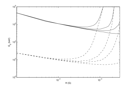
Figure 3: Limitations from radio observations for different values of time T passed since capture. In ascending order T = $1\times 10^{4}$, $5\times 10^{4}$, $10^{5}$, and $2\times 10^{5}$ years. Solid lines correspond to injection in form of delta-function, dashed lines correspond to power-law injection.

4 Constraints of the Model of Annihilation Emission

There are restrictions for our model which follow from radio and gamma-observations:

1. The flux of radio emission from the GC at present should not exceed the value of 1 kJy in the range 300 - 700 MHz (see, e.g., Mezger et al., 1996) that restricts the number of high energy positrons in the GC. The radius of high strength magnetic field sphere was taken to be $r_{H}=100$ pc;

2. The flux of annihilation emission observed at Earth from this region is $8\cdot 10^{-4}$ photons cm^-2s^-1 for the FWHM=$6\degr$ central region (Churazov et al., 2005);

3. The flux in the MeV energy range was measured by COMPTEL. As in Beacom and Yüksel (2006); Sizun et al. (2006) we accept that the flux of in-flight annihilation emission should not exceed the COMPTEL $2\sigma$ level of in the energy range 1-30 MeV, if it is due to in-flight annihilation.

These restrictions are presented in Table LABEL:param_st1.

Table 1: Constraints of the model

$\Phi_{\nu}(\nu=330$ MHz)	$F_{1-30~{}\mbox{MeV}}$	$I_{511~{}\mbox{keV}}$
$1.5\degr\times 0.5\degr$ region		FWHM =$6\degr$
$1$	$<2\sigma$ of COMPTEL	$8\cdot 10^{-4}$
kJy		ph cm-2s-1

5 Evolution of the Spectrum of Relativistic Positrons

We start from the spatially uniform model, which estimates the total flux of gamma-rays and radio emission (i.e. integrated over the volume of emission). The evolution of positron spectrum can be described by the equation

$$\frac{\partial N}{\partial t}+\frac{\partial}{\partial E}\left(\frac{dE}{dt}N\right)=Q(E,t)$$ (16)

where $dE/dt$ is the rate of synchrotron losses (see Eq. (7)). In case of instantaneous injection $Q(E,t)=N_{0}(E)\delta(t)$ where $N_{0}(E)$ is the injection spectrum of positron, the solution of this equation is

$$N=\frac{1}{|dE/dt|}N_{0}\left(\tau-t\right)$$ (17)

where

$$\tau=\int\limits_{E}^{\infty}\frac{dE}{|dE/dt|}$$ (18)

and $dE/dt$ is the rate of synchrotron or Coulomb losses.

In the high energy range, where the synchrotron losses are essential, the spectrum is

$$N=\frac{1}{(1-\beta Et)^{2}}N_{0}\left({\frac{E}{1-\beta Et}}\right)\theta(1-\beta Et)$$ (19)

We see that independent of the injection spectrum the maximum energy of positrons long after the injection is

$$E_{max}\simeq\frac{1}{\beta t}$$ (20)

where $t$ is time after the injection.

If the positrons are secondary, then their injection spectrum has a cut-off in the low energy range at $E_{\rm cut}\simeq 30$ MeV because of the threshold of $p-p$ reaction, and the energy distribution of positrons leaving the region of strong magnetic fields looks like a succession of separated bunches (see Fig.4). Here and below we take the injection spectrum of secondary positrons in the form

$$N_{0}(E)=A_{b}E^{-3}\theta(E-30~{}\mbox{MeV})$$ (21)

where $A_{b}\simeq 5.4\cdot 10^{58}$ MeV² gives the total number of injected positrons $\sim 3\cdot 10^{55}$, where the spectral index equals $-3$ as in the Galactic disk (see Berezinskii et al., 1990).

The bunch width is

$$\Delta E\sim\frac{1}{(\beta t)^{2}E_{\rm cut}}~{}\mbox{.}$$ (22)

The time duration of the bunch (characteristic time during which the bunch crosses any energy $E$ under the influence of synchrotron losses) is independent of $E$ and for the spectrum (21) equals

$$T_{b}=\frac{1}{\beta E_{\rm cut}}$$ (23)

that gives $T_{b}=3.6\cdot 10^{4}$yr for $E_{cut}=30$ MeV and $H=3$ mG. Subsequent bunches are separated from each other by the periods of $T_{i}\sim 10^{5}$ yr, the average periods of star capture.

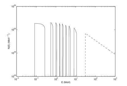
Figure 4: Spectrum of secondary positrons as a result of several successive capture events. The strength of magnetic field $H=3$ mG.

After the capture time equaled $10^{5}$ yr the maximum energy of positrons in the bunch shifts from $\infty$ to $E\simeq 10$ MeV (see Eq. (20), and there are no positrons in the energy range $E>10$ MeV while the energy range below 10 MeV contains permanently a number of bunches moving to the thermal region (see Fig. 4). Then we conclude that the spectrum of positrons in the range above 10 MeV is strongly non-stationary (shown by the dashed line in Fig. 4), as well as the emission generated by these particles. In contrary, the spectrum of positrons with energies $\la 10$ MeV (shown by the solid lines in Fig. 4) and the radiation produced by these positrons is quasi-stationary.

When the rate of synchrotron losses drops down with positron energy, the following evolution of positrons in the range $E<1$ MeV occurs under the influence of Coulomb losses. The rate of Coulomb losses is (Hayakawa, 1964; Ginzburg, 1989)

$${{dE}\over{dt}}=-{{2\pi e^{4}n}\over{mc\beta(E)}}\ln\Lambda$$ (24)

where $\log\Lambda$ is Coulomb logarithm, and $\beta(E)=v/c$. For lorenz-factor $\gamma=\frac{E}{mc^{2}}+1$ in a neutral medium

$$\log\Lambda\sim\log\left[(\gamma-1)(\gamma^{2}-1)\right]+20.5~{}\mbox{,}$$ (25)

while in completely ionized plasma

$$\log\Lambda\sim\log\left[\gamma/n\right]+73.6~{}\mbox{.}$$ (26)

6 Emission Produced by Non-Thermal Positrons

Relativistic positrons with energies higher than 10 MeV generate radio emission due to synchrotron losses and fluxes of in-flight annihilation and bremsstrahlung emission in the energy range above 10 MeV.

From Eqs. (14), (16) and (21) we calculated the time variations of radio emission from the GC at the frequency 330 MHz. The result of these calculations is shown in Fig. 5a. As it was expected at the very beginning, just after the injection of high energy positrons, the flux of radio emission is as high as $\Phi_{max}^{radio}\sim 3\cdot 10^{7}$ Jy, but its value decreases very rapidly with time. The present time corresponds to periods when the radio flux drops down below the level about 1 kJy (dotted line), as the observations require.

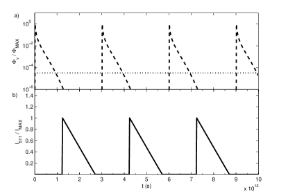
Figure 5: a) Time-variations of the radio flux from the GC. Here $\Phi_{max}^{radio}=3\cdot 10^{7}$ Jy. b) Annihilation flux variations from the GC in the framework of non-stationary model. Here $I_{max}^{511}=8\cdot 10^{-4}$ photons cm^-2s^-1.

The in-flight annihilation in the range 10-30 MeV is produced by positrons whose intensity is non-stationary. Therefore, this flux from the GC is time-variable (see Fig. 6)

Figure 6: Variations of the in-flight 10-30 MeV flux. The value of $F_{max}$ is presented in Table LABEL:outp_st.

On the contrary, the flux of in-flight annihilation in the ranges 1-3 and 3-10 MeV is almost stationary as expected.

The in-flight fluxes calculated for the cases of neutral and ionized medium and the COMPTEL $2\sigma$ levels are presented in Table LABEL:outp_st. The flux of the in-flight annihilation in the range 10-30 MeV presented in the table corresponds to the moment when the radio at 330 MHz drops to 1 kJy.

Table 2: Flux of in-flight annihilation in case of non-stationary annihilation (photons cm^-2s^-1).

Energy range (MeV)	COMPTEL $2\sigma$	Ionized	Neutral
1-3	$2\times 10^{-4}$	$1.2\times 10^{-5}$	$2.6\times 10^{-5}$
3-10	$9\times 10^{-5}$	$3.2\times 10^{-6}$	$3.6\times 10^{-6}$
10-30	$3\times 10^{-5}$	$3.7\times 10^{-7}$	$3.6\times 10^{-7}$

The bremsstrahlung flux in the energy range from 1 to 30 MeV was calculated for the cross-section from Haug (1997). Its values ranges from $5\times 10^{-7}$ in the range $1-3$ Mev to $3\times 10^{-7}$ at $3-10$ MeV and $1\times 10^{-7}$ at $10-30$ MeV. The flux units are the same as in Table LABEL:outp_st. One can see that bremsstrahlung doesn’t contribute much since lorentz-factor is rather small.

Table 3: Flux of in-flight annihilation in case of stationary annihilation (photons cm^-2s^-1).

Energy range (MeV)	COMPTEL $2\sigma$	Ionized	Neutral
1-3	$2\times 10^{-4}$	$4.6\times 10^{-5}$	$1\times 10^{-4}$
3-10	$9\times 10^{-5}$	$1.2\times 10^{-5}$	$1.4\times 10^{-5}$
10-30	$3\times 10^{-5}$	$1.5\times 10^{-6}$	$1.4\times 10^{-6}$

From these tables one can see that in all energy ranges the calculated in-flight flux is below the COMPTEL $2\sigma$ level. Therefore, in contrast to the conclusion of Beacom and Yüksel (2006) and Sizun et al. (2006), we find that there is no problem with the injection energy of positron in the model with strong magnetic field at GC. Corresponding combined spectra of in-flight annihilation and bremsstrahlung emission for magnetic fields in the range $0.1-3$ mG are shown in Fig. 7.

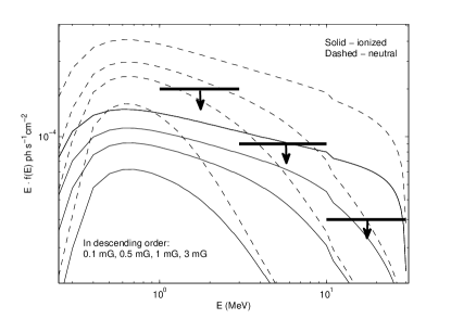
Figure 7: Combined in-flight annihilation and bremsstrahlung spectra for different values of magnetic field. COMPTEL limits are shown by heavy solid lines.

7 Annihilation Emission of Thermal Positrons

The characteristic time of annihilation for thermal positrons can be defined from

$$T_{ann}=\left[2\int\limits_{E_{T}}^{\infty}dE\sqrt{\frac{E}{\pi\Theta^{3}}}\exp\left(-\frac{E}{\Theta}\right)n\sigma(E)v\right]^{-1}$$ (27)

which is a function of the probability for thermal positrons to be in the energy range where the annihilation cross-section is high. Here temperature $\Theta\sim 1$ eV as it usually assumed. For the gas density $n\ga 1$ cm^-3 the annihilation time is about $\la 2.6\cdot 10^{4}$ yr (see Guessoum et al., 2005) which is smaller than the average time of star capture $T_{i}$ and the bunch time $T_{b}$. Then the process of annihilation emission is non-stationary since all positrons from a bunch annihilate during the time shorter than the period between two neighbour capture events.

The nondimensional equation for positrons has the form (here and below $f(p)$ is the density of positrons with momentum $p$)

$$\frac{\partial f}{\partial t}+\frac{\partial}{\partial p}\left(\left.\frac{dp}{dt}\right|_{C}f-D_{C}\frac{\partial f}{\partial p}\right)+$$

$$+n_{0}v\sigma_{if}f+n_{0}v\sigma_{ce}f=Q(p,t)$$ (28)

where $\left.dp/dt\right|_{C}$ and $D_{C}$ are the rate of Coulomb losses and the momentum diffusion due to Coulomb collisions. These two terms form the Maxwellian spectrum of thermal particles. The cross-sections $\sigma_{if}$ and $\sigma_{ce}$ denote the in-flight annihilation of fast positrons and the charge-exchange annihilation process of thermal particles.

The fluctuations of the annihilation flux expected in this case are shown in Fig. 5b. The maximum intensity of the annihilation emission corresponds to the value of $I_{max}^{511}=8\cdot 10^{-4}$ photons cm^-2s^-1. From this figure one can see that there are long periods of time when the annihilation flux reaches its maximum value while the radio emission is below the 1 kJy level as the observations require. It means that according to this model we see the annihilation flux from the bulge at its peak value.

If the gas density $n_{0}\la 0.25$ cm^-3 then the annihilation time $T_{ann}$ is larger than $T_{i}$ and the situation is quasi-stationary as follows from Eq. (27). Since the positrons from a single bunch do not annihilate completely for the period between two neighbour injections, then these positrons are accumulated in the thermal pool up to the level which provides a quasi-stationary rate of annihilation.

From Eq. (28) we calculated the flux of annihilation in the quasi-stationary case which is shown in Fig. 8 by the solid line. We see that fluctuations of the annihilation flux is much smaller than in the non-stationary case (see Fig. 5b).

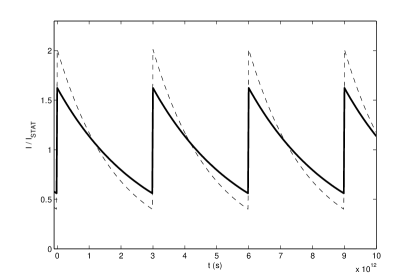
Figure 8: Variations of the annihilation flux from the GC in the framework of quasi-stationary model: solid line - without the effect of streaming instability, dashed line - with the effect of streaming instability. $I_{stat}$ is the average value of the annihilation flux.

The expected quasi stationary fluxes are presented in Table LABEL:outp_ststat. The bremsstrahlung flux in this case is: $2\times 10^{-6}$ at 1-3 MeV, $1\times 10^{-6}$ at 3-10 MeV, and $3\times 10^{-7}$ at 10-30 MeV. Again fluxes are below COMPTEL $2\sigma$.

An important conclusion from our calculations is that the only restriction of the model is the rate of synchrotron losses which should cool down positrons up to the energy $\la 10$ MeV for the time $\la 10^{5}$ yr, see Fig. 1. The regions of permitted values of positron injection energies derived from the COMPTEL restriction for different values of the magnetic field strength are shown in Fig. 9: the thick dashed line - ionized medium and the thick solid line - neutral medium. These region is below these lines. As one can see there are no restrictions for the injection energy from gamma-ray data if the magnetic field strength is high enough.

However, as we discussed already in the case of high magnetic field we have an additional restriction - the flux of radio emission at 330 MHz. The range of energy values which are derived from the radio data are shown by thin lines. In that part Fig. 9 is the same as Fig. 3: each line correspond to different value of period of injections (in ascending order T = $1\times 10^{4}$, $5\times 10^{4}$, $10^{5}$, and $2\times 10^{5}$ years). Thin solid lines correspond to injection in form of delta-function while thin dashed line correspond to power-law injection. Again as we mentioned already for strong magnetic field if period between two captures is long enough the injection energy can be very high.

So combining the gamma and radio data we conclude that the injection energy of positrons can be high if the model satisfies the tow conditions: the magnetic field strength is larger than 0.4 mG and the average period between two neighbour captures is longer than $10^{5}$ yr.

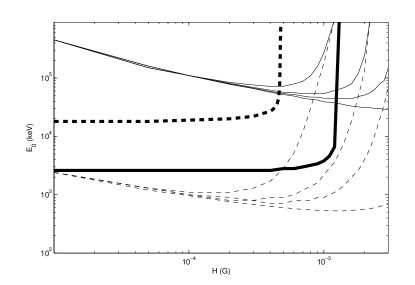
Figure 9: The multi-band limitations on the injection energy of positrons. Thin lines are the same as in Fig. 3. Thick dashed line represents limitations from COMPTEL energy range in case ionized medium. Thick solid lines represents limitations from COMPTEL energy range in case of neutral medium.

8 Landau Damping: Quasi-Stationary Model

As it follows from Eq. (19) when a bunch of MeV positrons escapes the strong magnetic field region into the surrounding medium the positron distribution looks like a two-peak function with one maximum at thermal energies and the other at the energies of the bunch (see Fig. 10). From the quasi-linear theory it follows that such a particle distribution is unstable (Artsimovich and Sagdeev, 1979, Ch.I, §1.16, p. 104, see also Lifshitz and Pitaevskii, 1981, Ch.III, §30, p.243), and the flux of fast particles excites effectively plasma waves due the streaming instability .

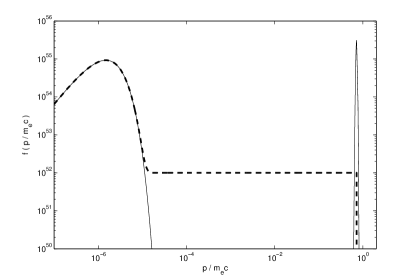
Figure 10: Transformation of the bunch spectrum by the streaming instability.

As a result a bunch of fast particles with the energy $E=E_{bunch}$ is transformed into ”a plateau” distribution in the energy region $E<E_{bunch}$. This process of the bunch smearing occurs due to resonant wave excitation ($v=\omega_{k}/k$, where $v$ if the particle velocity and $k$ is the wave number). This process is described as diffusion in the velocity space with the diffusion coefficient $D_{st}$ equaled

$$D_{st}\sim 4\pi^{2}\frac{e^{2}}{m^{2}}n_{b}m\frac{v^{2}}{\omega_{p}}\frac{v-v_{min}}{v_{max}}$$ (29)

where $n_{b}$ and $v_{max}$ is the density and the velocity of bunch particles, $v_{min}$ is about the velocity of thermal particles and $v$ is the current velocity of particles. The Langmuir frequency $\omega_{p}$ is

$$\omega_{p}=\sqrt{4\pi n_{0}e^{2}/m}$$ (30)

where $n_{0}$ is the density of background plasma. As numerical calculations showed (see, e.g. Artsimovich and Sagdeev, 1979, Ch.I, §1.16, p. 107) the bunch smearing was reached for several Langmuir times that in comparison with the model characteristic times is almost instantly. Calculations show that about one third of the bunch energy is transformed into the energy of excited plasma waves.

The nondimensional equation for nonthermal positrons has the form in this case

$$\frac{\partial f}{\partial t}+\frac{\partial}{\partial p}\left(\left.\frac{\partial p}{\partial t}\right|_{C}f-(D_{C}+D_{st})\frac{\partial f}{\partial p}\right)+$$

$$+n_{0}v\sigma_{if}f+n_{0}v\sigma_{ce}f=Q(p,t)$$ (31)

The expected variations of annihilation flux from the GC are shown in Fig. 8 by the dashed line. On can see that effect of streaming instability does not change the flux value significantly.

9 Spatial non-uniform model

We presented above our analysis of integrated fluxes from the GC. As we noticed mG magnetic fields occupy the inner sphere with the radius $r_{H}=100$ pc (i.e. its angular radius is $<1\degr$) while the FWHM of the annihilation emission is about $6\degr$. It means that in most of their lifetime positrons spend outside the central magnetic sphere. On the other hand, it follows from our analysis that positrons should be cooled down by strong magnetic fields up to the energy $\la 10$ MeV. These circumstances give restrictions for processes of positron propagation in the GC.

Spatial variation of the positron distribution function $N$ with propagation terms is described by the equation (see Berezinskii et al., 1990):

$$-\frac{1}{r^{2}}\frac{\partial}{dr}r^{2}D_{rr}\frac{\partial N}{\partial r}+\frac{\partial}{\partial E}\left[\frac{dE}{dt}N\right]+n\sigma vN=Q(E,r)~{}\mbox{,}$$ (32)

Here ${dE}/{dt}$ is the rate of total energy losses, and $D_{rr}$ is a spatial diffusion coefficient. We use a simple approximation for the spatial part of the injection function $Q(r)$, assuming that positron sources are uniformly distributed inside the sphere of the radius $r_{0}$, $Q(r,E)=Q(E)\theta(r_{0}-r)$. The function $Q(E)$ is given by Eq. (21) but with the coefficient $A_{b}\simeq 5\cdot 10^{46}$ MeV²/s as a result of averaging of injection processes over time (quasi-stationary injection).

The boundary condition are

$$\left(\nabla_{r}\cdot N\right)_{r=0}=0,~{}~{}~{}~{}~{}~{}~{}~{}~{}N_{r=\infty}=0$$ (33)

and

$$\left(\nabla_{p}\cdot N\right)_{E=0}=0$$ (34)

The loss term can be presented as

$$\frac{dE}{dt}=\left(dE/dt\right)_{coul}+\left(dE/dt\right)_{IC}+$$

$$+\left(dE/dt\right)_{synBK}\times\theta(r-r_{H})+$$

$$+\left(dE/dt\right)_{synS}\times\theta(r_{H}-r)~{}\mbox{,}$$ (35)

where $\left(dE/dt\right)_{synBK}$ is the rate of synchrotron losses in the outer sphere $r>r_{H}$ where the magnetic field strength equals $H\sim 10^{-5}$ G, and $\left(dE/dt\right)_{synS}$ is the rate of energy losses inside the central sphere $r<r_{H}$ losses in strong magnetic field $H=3$ mG.

The observed $6\degr$ FWHM of spatial distribution of annihilation emission corresponds to a sphere with the radius about 400 pc that requires the spatial diffusion coefficient be about $D_{rr}\sim 10^{28}$cm²s^-1. We notice here that propagation of MeV positrons in the GC is still very questionable (see e.g. Jean et al., 2009).

Fast cooling by synchrotron losses is possible only inside the sphere of strong magnetic field $r<r_{H}$. Therefore, the radius of source region should be quite small, $r_{0}<r_{H}$. Only in this case positrons are cooled to MeV energies by synchrotron losses and then fill the 400-pc sphere. In Fig. 11 we presented the calculated values of in-flight fluxes in the three COMPTEL energy ranges as a function of the source radius $r_{0}$. These fluxes are normalized to the COMPTEL 2$\sigma$ level presented in Table LABEL:outp_st. As one can see extended sources with $r_{0}r_{H}$ are unable to satisfy the COMPTEL restrictions if the injection energy is 30 MeV.

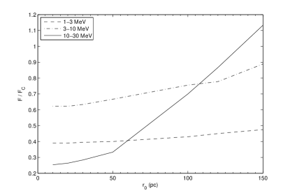
Figure 11: Variations of the in-flight flux as a function of the source region radius. Here $F_{c}$ is COMPTEL’s $2\sigma$ level.

10 Conclusion

We showed that:

• Unlike Beacom and Yüksel (2006) and Sizun et al. (2006), who restricted the injection energy of annihilating positrons at the value $1-7$ MeV, we show that under the condition of strong magnetic fields $H\ga 0.4$ mG in the Galactic center this value can be much larger. This extends significantly a class of models acceptable for explanation of the annihilation emission from the GC. However, the necessary condition in this case is that the positrons should be cooled down by the synchrotron losses up to the energy $\la 10$ MeV. Otherwise the expected radio flux and in-flight MeV emission from the GC exceed the level required from observations;

• The main restriction of this model follows from the value of observed radio flux from the GC which equals 1 kJy at the frequency 330 MHz. In order to satisfy this condition the peak of annihilation emission should be shifted in time to the moment when the radio flux falls down below the observed level;

• The energy spectrum of annihilating positrons looks like a number of bunches produced by subsequent capture events. In the case of the secondary origin of positrons the structure of the bunch spectrum is almost quasi-stationary in the energy range $\la 10$ MeV, and strongly non-stationary in the range above 10 MeV;

• On the other hand, the expected flux of the annihilation emission is quasi-stationary if the density of the background gas is $\la 0.25$ cm^-3.

• Time variations of the in-flight annihilation in the energy ranges 1-3, 3-10, and 10-30 MeV are quite small, and the important point is, their values are smaller than the COMPTEL $2\sigma$ level;

• Our calculations show that the size of the source region should be smaller than the radius of the sphere filled with strong magnetic field. Otherwise the in-flight flux exceeds the COMPTEL $2\sigma$ level.

It would be interesting to find traces of similar processes from other galaxies. If positrons injection is related to stellar capture events as it was suggested by Cheng et al. (2006) and Cheng et al. (2007) one can expect to find some traces of these processes in galactic nuclei with recent capture events in the form of high radio flux. However, galactic nuclei with high X-ray flux that indicates active accretion processes there do not show such a powerful radio emission (Wong et al., 2007). This is not surprising since the peak of radio emission is expected in our model some time after the capture. The delay time is about $10^{3}$ years as follows from the characteristic time of $p-p$ collisions which produce high energy electrons:

$$t_{pp}=(n\sigma_{pp}c)^{-1}\sim 10^{3}~{}\mbox{yr}$$ (36)

for the gas density of molecular clouds $n\sim 10^{4}$ cm^-3.

The flux of X-ray emission from the accretion disk scales with time like (Rees, 1988)

$$L_{x}\sim L_{edd}\left(\frac{t}{t_{min}}\right)^{-5/3}$$ (37)

where $t_{min}\simeq 0.2$ yr. So by the time radio emission peak reaches the X-ray emission decreases by a factor of $10^{6}$ from its initial value $\sim 10^{44}$ erg s^-1.

Thus, we expected a radio flux with the value $\sim 10^{8}$ Jy when the X-ray flux is already unseen. Galactic nuclei with such a brightness are commonly presented in the Universe (Hyeop Lee et al., 2009) and what is interesting that in some cases there is no activity in other energy ranges. That falls well into our model though these speculations cannot be considered as direct evidences in favor of our model.

DOC and VAD are partly supported by the RFBR grant 08-02-00170-a, the NSC-RFBR Joint Research Project RP09N04 and 09-02-92000-HHC-a and by the grant of a President of the Russian Federation ”Scientific School of Academician V.L.Ginzburg”. KSC is supported by a GRF grant of Hong Kong Government. CMK is supported by the Taiwan National Science Council grants NSC 96-2112-M-008-014-MY3 and NSC 98-2923-M-008-001-MY3. WHI is supported by the Taiwan National Science Council grants NSC 96-2752-M-008-011-PAE and NSC 96-2111-M-008-010.

We would like to mention that the referee’s report was very useful for us, and we thank him for his comments. DOC and VAD thank the Institute of Astronomy of NCU for hospitality during their stay there.

References

- Abraham et al. (2007) Abraham J., Abreu, P., Aglietta, M., et al. [Pierre Auger Collaboration], 2007, Sci, 318, 938
- Aharonian and Atoyan (2000) Aharonian F. A., & Atoyan A. M., 2000, A&A, 362, 937
- Artsimovich and Sagdeev (1979) Artsimovich, L. A., and Sagdeev, R. Z. 1979, Plasma physics for physicists, Moscow, Atomizdat (in Russian)
- Bandyopadhyay et al. (2007) Bandyopadhyay, R. M., Silk, J., Taylor, J.E., & Maccarone, Th.J., 2009, MNRAS, 392, 1115
- Beacom et al. (2005) Beacom J. F., Bell N. F., Bertone G., 2005, PhysRev Lett, 95, 171301
- Beacom and Yüksel (2006) Beacom J. F. & Yüksel H., 2006, PhysRev Lett, 97, 071102
- Berezinskii et al. (1990) Berezinskii, V. S., Bulanov, S. V., Dogiel, V. A., Ginzburg, V. L., and Ptuskin, V. S. 1990, Astrophysics of Cosmic Rays, ed. V.L.Ginzburg, (Norht-Holland, Amsterdam)
- Boehm et al (2004) Boehm C., Ensslin T. A., Silk, J., 2004, JPhG, 30, 279
- Bussard et al. (1979) Bussard, R. W., Ramaty, R., & Drachman, R. J. 1979, ApJ, 228, 928
- Cheng et al. (2006) Cheng, K. S., Chernyshov, D. O., & Dogiel, V. A., 2006, ApJ, 645, 1138.
- Cheng et al. (2007) Cheng K. S., Chernyshov D. O., & Dogiel V. A., 2007, A&A, 473, 351
- Chernyshov et al. (2008) Chernyshov, D. O., Cheng, K.-S., Dogiel, V. A., 2008, Proceedings of Science, (7th INTEGRAL Workshop, September 8-11, 2008, Copenhagen, Denmark)
- Churazov et al. (2005) Churazov E., Sunyaev R., Sazonov S., Revnivtsev M., & Varshalovich, D., 2005, MNRAS, 1377, 1386
- Ferriere (2009) Ferriere, K., 2009, A&A, 505, 1183
- Ginzburg (1989) Ginzburg, V.L. 1989, Applications of Electrodynamics in Theoretical Physics and Astrophysics, Gordon and Brech Science Publication.
- Guessoum et al. (2005) Guessoum, N., Jean, P. & Gillard, W. 2005, A&A, 436, 171
- Haug (1997) Haug E., 1997, A&A, 326, 417
- Hayakawa (1964) Hayakawa, S. 1964, Cosmic Ray Physics, (ed R.E. Marshak), Interscience Monographs
- Higdon et al (2009) Higdon J. C., Lingenfelter R. E., Rothschild R. E., 2009, ApJ, 698, 350
- Istomin & Sol (2009) Istomin Y. N., & Sol H., 2009, Ap&SS, 321, 57I
- Jean et al. (2006) Jean P., Knödlseder J., Gillard W. et al. 2006, A&A, 445, 579
- Jean et al. (2009) Jean, P.; Gillard, W.; Marcowith, A.; Ferriere, K. 2009, astro-ph 0909.4022, to be published in A&A
- Knödlseder et al. (2005) Knödlseder J., Jean, P., Lonjou, V. et al., 2005, A&A, 441, 513
- Koyama et al. (2007) Koyama K., Hyodo, Y., Inui, T.et al., 2007, PASJ, 59, S245
- Koyama et al. (1996) Koyama K., Maeda Y., Sonobe T. et al. 1996, PASJ, 48, 249
- LaRosa et al. (2005) LaRosa T. N., Brogan C. L., Shore S. N. et al., 2005, ApJ, 626, L23
- Hyeop Lee et al. (2009) Hyeop Lee J., Lee M. G., Park C., Choi Y. Y., 2009, arXiv:0909.3541v2
- Lifshitz and Pitaevskii (1981) Lifshitz, E. M. & Pitaevskii, L. P. 1981, Physical kinetics, Course of theoretical physics, Oxford: Pergamon Press
- Mezger et al. (1996) Mezger P. G., Duschl W. J., & Zylka R., 1996, A&A Rev, 7, 289
- Morris (2006) Morris M., 2006, Journal of Physics: Conference Series, 54, 1, 1
- Morris and Serabyn (1996) Morris, M. & Serabyn, E. 1996, ARA&A, 34, 645
- Muno et al. (2004) Muno M. P. et al., 2004, ApJ, 613, 1179
- Plante, Lo and Crutcher (1995) Plante R. L, Lo K. Y, Crutcher R. M., ApJ, 445, L113
- Porter et al. (2008) Porter T. A., Moskalenko I. V., Strong A.W., Orlando E., Bouchet L., 2008, ApJ, 682, 400
- Prantzos (2006) Prantzos N., 2006, A&A, 449, 869
- Rees (1988) Rees M. J., 1998, Nature, 333, 523
- Sizun et al. (2006) Sizun P., Cassé M. & Schanne S., 2006, PhysRevD, 74, 063514
- Spergel and Blitz (1992) Spergel D. N., Blitz L., 1992, Nat, 357, 665
- Strong et al. (2005) Strong A. W., Diehl R., Halloin H. et al. 2005, A&A, 444, 495
- Strong et al. (1998) Strong A.W., Bloemen H., Diehl R., Hermsen W., & Schönfelder V., 1998, in proceeding of 3rd INTEGRAL Workshop
- Yusef-Zadeh et al. (1999) Yusef-Zadeh F., Roberts D. A., Goss W. M., Frail D. A. and Green A. J., 1999, ApJ, 512, 230
- Yusef-Zadeh, Hewitt and Cotton (2004) Yusef-Zadeh F., Hewitt J. W., Cotton W., 2004, ApJS, 155, 421
- Totani (2006) Totani T., 2006, PASJ, 58, 965
- Weidenspointner et al. (2008) Weidenspointner G., Skinner, G., Jean, P. et al., 2008, Nature, 451, 159
- Wong et al. (2007) Wong A. Y. L., Huang Y. F., Cheng K. S., 2007, A&A, 472, 93