Measures of lexical distance between languages

Abstract

The idea of measuring distance between languages seems to have its roots in the work of the French explorer Dumont D’Urville Urv . He collected comparative words lists of various languages during his voyages aboard the Astrolabe from 1826 to 1829 and, in his work about the geographical division of the Pacific, he proposed a method to measure the degree of relation among languages. The method used by modern glottochronology, developed by Morris Swadesh in the 1950s, measures distances from the percentage of shared cognates, which are words with a common historical origin. Recently, we proposed a new automated method which uses normalized Levenshtein distance among words with the same meaning and averages on the words contained in a list. Recently another group of scholars Bak ; Hol proposed a refined of our definition including a second normalization. In this paper we compare the information content of our definition with the refined version in order to decide which of the two can be applied with greater success to resolve relationships among languages.

1 Introduction

Glottochronology tries to estimate the time at which languages diverged with the implicit assumption that vocabularies change at a constant average rate. The idea is to consider the percentage of shared cognates in order to compute the distance between pairs of languages Sw . These lexical distances are assumed to be, on average, logarithmically proportional to divergence times. In fact, changes in vocabulary accumulate year after year and two languages initially similar become more and more different. A recent example of the use of Swadesh lists and cognates to construct language trees are the studies of Gray and Atkinson GA and Gray and Jordan GJ .

We recently proposed an automated method which uses Levenshtein distance among words in a list SP ; SP2 . To be precise, we defined the lexical distance of two languages by considering a normalized Levenshtein distance among words with the same meaning and averaging on all the words contained in a Swadesh list. The normalization is extremely important and no reasonable results can be found without. Then, we transformed the lexical distances in separation times. This goal was reached by a logarithmic rule which is the analogous of the adjusted fundamental formula of glottochronology ST . Finally, the phylogenetic tree could be straightforwardly constructed.

In SP ; SP2 we tested our method by constructing the phylogenetic trees of the Indo-European and the Austronesian groups.

Almost at the same time, the above described automated method was used and developed by another large group of scholars Bak ; Hol . They placed the method at the core of an ambitious project, the ASJP (The Automated Similarity Judgment Program). In their work they proposed a refined of our definition including a second normalization in the definition of lexical distance.

The goal of this paper is to compare the information content of the two definitions in order to decide which of the two can be applied with greater success to resolve relationships among languages.

Before tackling this problem we sketch our definition of lexical distance and the modification proposed in Bak ; Hol which is a refinement including a second normalization. Then we compare the information content of the two definitions and give our conclusion.

2 Lexical distance

Our definition of lexical distance between two words is a variant of the Levenshtein distance which is simply the minimum number of insertions, deletions, or substitutions of a single character needed to transform one word into the other. Our definition is taken as the Levenshtein distance divided by the number of characters of the longer of the two compared words. More precisely, given two words $\alpha_{i}$ and $\beta_{j}$ their lexical distance $D(\alpha_{i},\beta_{j})$ is given by

$$D(\alpha_{i},\beta_{j})=\frac{D_{l}(\alpha_{i},\beta_{j})}{L(\alpha_{i},\beta_{j})}$$ (1)

where $D_{l}(\alpha_{i},\beta_{j})$ is the Levenshtein distance between the two words and $L(\alpha_{i},\beta_{j})$ is the number of characters of the longer of the two words $\alpha_{i}$ and $\beta_{j}$. Therefore, the distance can take any value between 0 and 1. Obviously $D(\alpha_{i},\alpha_{i})=0$ .

The normalization is an important novelty and it plays a crucial role; no sensible results can been found withoutSP ; SP2 .

We use distance between pairs of words, as defined above, to construct the lexical distances of languages. For any pair of languages, the first step is to compute the distance between words corresponding to the same meaning in the Swadesh list. Then, the lexical distance between each languages pair is defined as the average of the distance between all wordsSP ; SP2 . As a result we have a number between 0 and 1 which we claim to be the lexical distance between two languages.

Assume that the number of languages is $N$ and the list of words for any language contains $M$ items. Any language in the group is labeled a Greek letter (say $\alpha$) and any word of that language by $\alpha_{i}$ with $1\leq i\leq M$. Then, two words $\alpha_{i}$ and $\beta_{j}$ in the languages $\alpha$ and $\beta$ have the same meaning if $i=j$.

Then the distance between two languages is

$$D(\alpha,\beta)=\frac{1}{M}\sum_{i}D(\alpha_{i},\beta_{i})$$ (2)

where the sum goes from 1 to $M$. Notice that only pairs of words with same meaning are used in this definition. This number is in the interval [0,1], obviously $D(\alpha,\alpha)=0$.

The results of the analysis is a $N\times N$ upper triangular matrix whose entries are the $N(N-1)$ non trivial lexical distances $D(\alpha,\beta)$ between all pairs in a group. Indeed, our method for computing distances is a very simple operation, that does not need any specific linguistic knowledge and requires a minimum of computing time.

A phylogenetic tree could be constructed from the matrix of lexical distances $D(\alpha,\beta)$, but this would only give the topology of the tree whereas the absolute time scale would be missing. Therefore, we perform SP ; SP2 a logarithmic transformation of lexical distances which is the analogous of the adjusted fundamental formula of glottochronologyST . In this way we obtain a new $N\times N$ upper triangular matrix whose entries are the divergence times between all pairs of languages. This matrix preserves the topology of the lexical distance matrix but it also contains the information concerning absolute time scales. Then, the phylogenetic tree can be straightforwardly constructed.

In SP ; SP2 we tested our method constructing the phylogenetic trees of the Indo-European group and of the Austronesian group. In both cases we considered $N=50$ languages. The databasefootnote that we used in SP ; SP2 is composed by $M=200$ words for any language. The main source for the database for the Indo-European group is the file prepared by Dyen et al. in D . For the Austronesian group we used as the main source the lists contained in the huge database in NZ .

3 A second normalization

A further modification has been proposed by Bak ; Hol in order to avoid possible similarity which could arose from accidental relative orthographical similarity of languages.

Let us first define the global distance between languages $\alpha$ and $\beta$ as

$$\Gamma(\alpha,\beta)=\frac{1}{M(M-1)}\sum_{i\neq j}D(\alpha_{i},\beta_{j})$$ (3)

where the sum goes on all $M(M-1)$ pairs of words corresponding to different meanings in the two lists ($M^{2}$ is the total number of pairs and $M$ is the number of pairs with same meaning).

This quantity measures a distance of the vocabulary of the two languages, without comparing words with same meaning. In other words, it only account for general similarities in the frequency and ordering of characters. The point is that, at this stage, we don’t know if $\Gamma(\alpha,\beta)$ carries informations or only depends on accidental similarities.

Assuming the second point of view, it is reasonable to define, according to Bak ; Hol , a bi-normalized lexical distance as follows:

$$D_{s}(\alpha,\beta)=\frac{D(\alpha,\beta)}{\Gamma(\alpha,\beta)}$$ (4)

This second normalization should cancel the effects of accidental orthographical similarities between the two languages. Notice that while by definition $D(\alpha,\alpha)=D_{s}(\alpha,\alpha)=0$, in all real cases $\Gamma(\alpha,\alpha)\neq 0$.

We would like to stress that the idea of the proposed second normalization turns to be correct only if $\Gamma(\alpha,\beta)$ is uncorrelated with the lexical distance between languages $\alpha$ and $\beta$. In this case, in fact, it has vanishing information concerning their relationship. On the contrary, if it is positively correlated with the distance between the two languages, one can conclude that it contains some information that can be usefully exploited.

4 Comparison of different definitions

In order to decide which definition is better to use, $D(\alpha,\beta)$ or $D_{s}(\alpha,\beta)$, we have to see if $\Gamma(\alpha,\beta)$ is positively correlated with these distances. In case it is not, we will decide to use $D_{s}(\alpha,\beta)$ since we eliminate errors due to accidental similarities between vocabularies. On the contrary, if it is positively correlated, we would conclude that $\Gamma(\alpha,\beta)$ carries some positive information about the degree of similarity of the two languages. In this second case, two languages will be, in average, closer for smaller $\Gamma(\alpha,\beta)$ and we would decide to use $D(\alpha,\beta)$ since it incorporates the information contained in $\Gamma(\alpha,\beta)$.

In order to compute the correlation between distance and $\Gamma(\alpha,\beta)$ we proceed as follows: first we define for a generic function $f(\alpha,\beta)$ the average $<$$f$$>$ on all possible values of $\alpha$ and $\beta$ as follows

$$<\!\!f\!\!>=\frac{1}{N^{2}}\sum_{\alpha,\beta}f(\alpha,\beta)$$ (5)

which is the average value of the function $f(\alpha,\beta)$ in a linguistic group. Then, we define the correlation between $D(\alpha,\beta)$ and $\Gamma(\alpha,\beta)$ in a standard way as

$$C(\Gamma,D)=\frac{<\!\!(\Gamma-<\!\!\Gamma\!\!>)(D-<\!\!D\!\!>)\!\!>}{(<\!\!(\Gamma-<\!\!\Gamma\!\!>)^{2}\!\!><\!\!(D-<\!\!D\!\!>)^{2}\!\!>)^{\frac{1}{2}}}$$ (6)

The result is that the correlation in the Indo-European group is $0.59173$ while in the Austronesian group is $0.46032$. In both cases it is a quite high positive value (correlation may take any value between -1 and 1) and we conclude that eventual vocabulary similarities accounted by $\Gamma(\alpha,\beta)$ carry information and are not at all accidental. The week point is that we have checked correlation against $D(\alpha,\beta)$ which, at least from the point of view of the proponents of the second normalization, linearly incorporates $\Gamma(\alpha,\beta)$ since $D(\alpha,\beta)=\Gamma(\alpha,\beta)D_{s}(\alpha,\beta)$.

From this point of view our result is not so astonishing. Nevertheless, we can also compute the correlation between the bi-normalized distance $D_{s}(\alpha,\beta)$ and $\Gamma(\alpha,\beta)$. The definition is the same as (6) with $D_{s}$ substituting $D$. We obtain that the correlation $C(\Gamma,D_{s})$ in the Indo-European group is $0.54713$ while in the Austronesian group is $0.40169$. These two data, although slightly smaller than the previous ones, are still quite high and confirm that $\Gamma(\alpha,\beta)$ contains positive information. In other words, closer languages, both in the sense of a smaller $D(\alpha,\beta)$ and a smaller $D_{s}(\alpha,\beta)$, will have on average smaller $\Gamma(\alpha,\beta)$.

We remark that the same correlation coefficients, both for $D$ and $D_{s}$, comes out, if the average (5) is computed negletting the pairs were the same greek index is repeated.

In order to complete our analysis we plot, only for the Austronesian languages group, $\Gamma(\alpha,\beta)$ as a function of $D(\alpha,\beta)$ (Fig. 1 left) and as a function of $D_{s}(\alpha,\beta)$ (Fig. 1 right). Any point in the figures represents a pair of languages. In both cases we perceive the positive correlation which is evidenced by the best linear fits.

We remark that the points which lie on the vertical axes at the 0 distance value correspond, in both figures, to pairs for which the same language is compared. For these points the $D(\alpha,\alpha)=D_{s}(\alpha,\alpha)$ are all equal to 0 while the $\Gamma(\alpha,\alpha)$ are positive. It is easy to see that the self-distances accounted by the $\Gamma(\alpha,\alpha)$, which compare words with different meaning in the same language, are, on average, smaller than the $\Gamma(\alpha,\beta)$ which compare words with different meaning in two different languages. This fact confirms that the information carried by $\Gamma(\alpha,\beta)$ is positive.

In other words, closer related languages, not only have more similar words corresponding to the same meaning, but the general occurrence and ordering of characters in words is more similar.

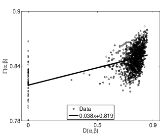
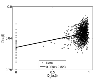
Figure 1: Global distance $\Gamma(\alpha,\beta)$ versus lexical distance $D(\alpha,\beta)$ (left) and versus bi-normalized distance $D_{s}(\alpha,\beta)$ (right) for Austronesian languages. The positive correlation is evidenced by the best linear fits. The points which lie on he vertical axes at the 0 distance value correspond to pairs for which the same language is compared. For these points $D(\alpha,\alpha)=D_{s}(\alpha,\alpha)$ while $\Gamma(\alpha,\alpha)\neq 0$.

5 Conclusions

In this work we have analyzed two different possibilities for the definition of automated languages distance. More precisely, starting from a Levenshtein distance, we have analyzed two possible normalizations. The choice between them is only made by using statistical arguments.

Our conclusion is that it is preferable to use the single normalization definition of distance $D(\alpha,\beta)$, otherwise a part of the information about affinities of languages is lost. In fact, our analysis shows that closer related languages have smaller global distance. This means that not only they have more similar words for the same meaning, but the general occurrence and ordering of characters in words is more similar.

References

- (1) D. Bakker, C. H. Brown, P. Brown, D. Egorov, A. Grant, E. W. Holman, R. Mailhammer, A. M ller, V. Velupillai and S. Wichmann Adding typology to lexicostatistics: a combined approach to language classification, Linguistic Typology (in press)
- (2) D. D’Urville, Sur les îles du Grand Océan, Bulletin de la Société de Goégraphie 17, (1832), 1-21.
- (3) I. Dyen , J.B. Kruskal and P. Black, FILE IE-DATA1. Available at (1997)
- (4) R. D. Gray and Q. D. Atkinson, Language-tree divergence times support the Anatolian theory of Indo-European origin. Nature 426, (2003), 435-439
- (5) R. D. Gray and F. M, Jordan, Language trees support the express-train sequence of Austronesian expansion. Nature 405, (2000), 1052-1055
- (6) S. J. Greenhill, R. Blust, and R.D. Gray, The Austronesian Basic Vocabulary Database, http://language.psy.auckland.ac.nz/austronesian, (2003-2008).
- (7) E. W. Holman, S. Wichmann, C. H. Brown, V. Velupillai, A. Muller and D. Bakker, Explorations in automated lexicostatistics Folia Linguistica 42.2, (2008), 331-354 ics, 26, (2000), 144-146.
- (8) F. Petroni and M. Serva, Languages distance and tree reconstruction. Journal of Statistical Mechanics: theory and experiment, (2008), P08012.
- (9) M. Serva and F. Petroni, Indo-European languages tree by Levenshtein distance. EuroPhysics Letters 81, (2008), 68005
- (10) S. Starostin, Comparative-historical linguistics and Lexicostatistics. In: Historical linguistics and lexicostatistics. Melbourne, (1999), 3-50.
- (11) M. Swadesh, Lexicostatistic dating of prehistoric ethnic contacts. Proceedings American Philosophical Society, 96, (1952), 452-463.
- (12) The database, modified by the Authors, is available at the following web address: http://univaq.it/serva/languages/languages.html. Readers are welcome to modify, correct and add words to the database.