Play building blocks on population distribution of multilevel superconducting flux qubit with quantum interference

Abstract

Recent experiments on Landau-Zener interference in multilevel superconducting flux qubits revealed various interesting characteristics, which have been studied theoretically in our recent work[PRB $\mathbf{79},094529$, (2009)] by simply using rate equation method. In this note we extend this method to the same system but with larger driving amplitude and higher driving frequency. The results show various anomalous characteristics, some of which have been observed in a recent experiment.

In this note, we show the anomalous characteristics in population distribution of superconducting flux qubit under driving fields with large amplitude($A$) and high frequency($\omega$). For a field-driving multilevel flux qubit with diabatic quantum states $|i,L\rangle$(left well, i=0,1,2…) and $|j,R\rangle$(right well, j=0,1,2,…), Berns ; Oliver the Landau-Zener transition rate between $|i,L\rangle$ and $|j,R\rangle$ is:Wen

$$W_{ij}(\epsilon_{ij},A)=\frac{\Delta_{ij}^{{2}}}{2}\sum_{n}\frac{\Gamma_{2}J^{2}_{n}(x)}{(\epsilon_{ij}-n\omega)^{2}+\Gamma^{2}_{2}},$$ (1)

where $\Delta_{ij}$ is the avoided crossing between states $|i,L\rangle$ and $|j,R\rangle$, ,$\epsilon_{ij}$ is the dc energy detuning from the corresponding avoided crossing $\Delta_{ij}$, $\Gamma_{2}=1/T_{2}$ is the dephasing rate and $J_{n}(x)$ are Bessel functions of the first kind with the argument $x=A/\omega$.

The time evolution of population for state $|i,L\rangle$ can be described byWen

$$\dot{P}_{i,L} = -\sum_{j}W_{ij}P_{i,L}+\sum_{j}W_{ij}P_{j,R}$$ (2)

$$-\sum_{i^{\prime}}\Gamma_{i\to i^{\prime}}P_{i,L}+\sum_{i^{\prime}}\Gamma_{i^{\prime}\to i}P_{i^{\prime},L}$$

$$-\sum_{j}\Gamma_{i\to j}P_{i,L}+\sum_{j}\Gamma_{j\to i}P_{j,R},$$

where $\Gamma_{i\to i^{\prime}}$ is the intrawell relaxation rate from $|i,L\rangle$ to $|i^{\prime},L\rangle$ , and $\Gamma_{i\to j}$ is the interwell relaxation rate from $|i,L\rangle$ to $|j,R\rangle$. The time evolution of population for state $|j,R\rangle$ can be obtained in the same way. In the stationary case, we have $\dot{P}_{i,L(R)}=0$. The qubit population distribution can be easily obtained by

$$P_{L(R)}=\sum_{i(j)}P_{i,L(j,R)}$$ (3)

Based on Eq.(1-3), we can play building blocks. Eq.(1) serves as the basic building block, Eq.(2) serves as the rule of the game, and Eq.(3) shows the total pattern. By adjusting the frequency $\omega$ and dephasing rate $\Gamma_{2}$ in Eq.(1), we can choose different kinds of building blocks. Therefore, kinds of interesting patterns can be constructed. As shown in Fig. 1, the diamond patterns observed in recent experimentsBerns ; Oliver are well obtained based on Eq.(1-3) with experimental parameters.

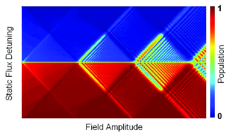
Figure 1: Calculated qubit population versus flux detuning and driving amplitude. The parameters are from experiments.Berns The dephasing rate is $\Gamma_{2}/2\pi=0.5$GHz and the driving frequency is $\omega/2\pi=160$MHz.

By increasing the driving frequency continually, we can obtain more interesting patterns. As shown in Fig. 2, with the parameters in a recent experiment where the driving frequency is much higher($\omega/2\pi$$\sim$10GHz), we can obtain various anomalous patterns, some of which have been demonstrated by experiments.Wang

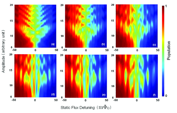
Figure 2: Calculated qubit population versus flux detuning and driving amplitude. The simulation parameters are from experiments.Wang The driving frequencies($\omega/2\pi$) are (a)5GHz, (b)8GHz, (c)11GHz, (d)13GHz, (e)15GHz, and (f)17GHz, respectively.

References

- (1) D. M. Berns, M. S. Rudner, S. O. Valenzuela, K. K. Berggren, W. D. Oliver, L. S. Levitov, and T. P. Orlando, Nature (London) 455, 51 (2008).
- (2) W. D. Oliver and S. O. Valenzuela, Quantum Inf. Process. 8, 261 (2009).
- (3) X. Wen and Y. Yu Phys. Rev. B 79, 094529 (2009).
- (4) Y. Wang, S. Cong, X. Wen, C. Pan, G. Sun, J. Chen, L. Kang, W. Xu, Y. Yu, and P. Wu, arXiv:0912.0995.