Qualitative Robustness of Support Vector Machines

Zusammenfassung

Support vector machines have attracted much attention in theoretical and in applied statistics. Main topics of recent interest are consistency, learning rates and robustness. In this article, it is shown that support vector machines are qualitatively robust. Since support vector machines can be represented by a functional on the set of all probability measures, qualitative robustness is proven by showing that this functional is continuous with respect to the topology generated by weak convergence of probability measures. Combined with the existence and uniqueness of support vector machines, our results show that support vector machines are the solutions of a well-posed mathematical problem in Hadamard’s sense.

• 2000 AMS Classification numbers:  62G08, 62G35

• KEYWORDS:  Nonparametric regression, classification, machine learning, support vector machines, qualitative robustness

1 A Long Introduction

Two of the most important topics in statistics are classification and regression. There, it is assumed that the outcome $y\in\mathcal{Y}$ of a random variable $Y$ (output variable) is influenced by an observed value $x\in\mathcal{X}$ (input variable). On the basis of a finite data set $\big{(}(x_{1},y_{1}),\dots,(x_{n},y_{n})\big{)}\in(\mathcal{X}\times\mathcal{Y})^{n}$ , the goal is to find an “optimal” predictor $f:\mathcal{X}\rightarrow\mathcal{Y}$ which makes a prediction $f(x)$ for an unobserved $y$ . In parametric statistics, a signal plus noise relationship

$$y\;=\;f_{\theta}(x)+\varepsilon$$

is often assumed, where $f_{\theta}$ is precisely known except for a finite parameter $\theta\in\mathds{R}^{p}$ and $\varepsilon$ is an error term (generated from a Normal distribution). In this way, the goal of estimating an “optimal” predictor (which can be any function $f:\mathcal{X}\rightarrow\mathcal{Y}$) reduces to the much simpler task of estimating the parameter $\theta\in\mathds{R}^{p}$ . Since, in many applications, such strong assumptions can hardly be justified, nonparametric regression has been developed which avoids (or at least considerably weakens) such assumptions. In statistical machine learning, the method of support vector machines has been developed as a method of nonparametric regression; see e.g., Vapnik (1998), Schölkopf and Smola (2002), and Steinwart and Christmann (2008). There, the estimation of the predictor (called empirical SVM) is a function $f$ which solves the minimization problem

$$\min_{f\in H}\,\frac{1}{n}\sum_{i=1}^{n}L\big{(}(x_{i},y_{i},f(x_{i})\big{)}\,+\,\lambda\|f\|_{H}^{2}\;,$$ (1)

where $H$ is a certain function space $H$ . The first term in (1) is the empirical mean of the losses caused by the predictions $f(x_{i})$ and the second term penalizes the complexity of $f$ in order to avoid overfitting, $\lambda$ is a positive real number, and the space $H$ is a reproducing kernel Hilbert space (RKHS) which consists of functions $f:\mathcal{X}\rightarrow\mathds{R}$ .

Since the arise of robust statistics (Tukey (1960), Huber (1964)), it is well-known that imperceptible small deviations of the real world from model assumptions may lead to arbitrarily wrong conclusions. While many practitioners are aware of the need for robust methods in classical parametric statistics, it is quite often overseen that robustness is also a crucial issue in nonparametric statistics. For example, the sample mean can be seen as a nonparametric procedure which is non-robust since it is extremely sensitive to outliers: Let $X_{1},\dots,X_{n}$ be i.i.d. random variables with unknown distribution $\mathrm{P}$ and the task is to estimate the expectation of $\mathrm{P}$ . If the observed data are really generated by the ideal $\mathrm{P}$ (and if expectation and variance of $\mathrm{P}$ exist), then the sample mean is the optimal estimator. However, it frequently happens in the real world that, due to outliers or small model violations, the observed data are not generated by the ideal $\mathrm{P}$ but by another distribution $\mathrm{P}^{\prime}$ . Even if $\mathrm{P}^{\prime}$ is close to the ideal $\mathrm{P}$ , the sample mean may lead to disastrous results. Detailed descriptions and some examples of such effects are given, e.g., in Tukey (1960), Huber (1964), and Huber (1981, § 1.1).

In nonparametric regression, similar effects can occur. There, it is often assumed that $(X_{1},Y_{1}),\dots,(X_{n},Y_{n})$ are i.i.d. random variables with unknown distribution $\mathrm{P}$ . This distribution $\mathrm{P}$ determines in which way the output variable $Y_{i}$ is influenced by the input variable $X_{i}$. However, estimating a predictor $f:\mathcal{X}\rightarrow\mathcal{Y}$ can be severely distorted if the observed data $(x_{1},y_{1}),\dots,(x_{n},y_{n})$ are – just as usual – not generated by $\mathrm{P}$ but by another distribution $\mathrm{P}^{\prime}$ which may be close to the ideal $\mathrm{P}$. In order to safeguard from severe distortions, an estimator $S_{n}$ should fulfill some kind of continuity: If the real distribution $\mathrm{P}^{\prime}$ is close to the ideal distribution $\mathrm{P}$ , then the distribution of the estimator $S_{n}$ should hardly be affected (uniformly in the sample sizes $n\in\mathds{N}$). This kind of robustness is called qualitative robustness and has been formalized in Hampel (1968, 1971) for estimators taking values in $\mathds{R}^{p}$ .

In order to study this notion of robust statistics for support vector machines, we need a generalization given by Cuevas (1988) of this formalization because, here, the values of the estimator are functions $f:\mathcal{X}\rightarrow\mathcal{Y}$ which are elements of a (typically infinite dimensional) Hilbert space $H$ . In case of support vector machines, the estimators

$$S_{n}\;:\;\;(\mathcal{X}\times\mathcal{Y})^{n}\;\rightarrow\;H$$

can be represented by a functional

$$S\;:\;\;\mathcal{M}_{1}(\mathcal{X}\times\mathcal{Y})\;\rightarrow\;H$$

on the set $\mathcal{M}_{1}(\mathcal{X}\times\mathcal{Y})$ of all probability measures on $\mathcal{X}\times\mathcal{Y}$ :

$$S_{n}\big{(}(x_{1},y_{1}),\dots,(x_{n},y_{n})\big{)}\;=\;S\Bigg{(}\frac{1}{n}\sum_{i=1}^{n}\delta_{(x_{i},y_{i})}\Bigg{)}$$

for every $(x_{1},y_{1}),\dots,(x_{n},y_{n})\in\mathcal{X}\times\mathcal{Y}$ where $\frac{1}{n}\sum_{i=1}^{n}\delta_{(x_{i},y_{i})}$ is the empirical measure and $\delta_{(x_{i},y_{i})}$ denotes the Dirac measure in $(x_{i},y_{i})$ . It is shown by Cuevas (1988) that, in such cases, the qualitative robustness of a sequence of estimators $(S_{n})_{n\in\mathds{N}}$ follows from the continuity of the functional $S$ (with respect to the topology of weak convergence of probability measures). While quantitative robustness of support vector machines has already been investigated by means of Hampel’s influence functions and bounds for the maxbias in Christmann and Steinwart (2007)) and by means of Bouligand influence functions in Christmann and Van Messem (2008), results about qualitative robustness of support vector machines have not been published so far. The goal of this paper is to fill this gap on research on qualitative robustness of support vector machines.

The structure of the article is as follows: In the following Section 2, we recall the basic setup concerning support vector machines, define the functional $S$ which represents the SVM-estimators $S_{n}$ , $n\in\mathds{N}$, and quote the mathematical definition of qualitative robustness. In Section 3, we show that the functional $S$ of support vector machines is, in fact, continuous under very mild assumptions (Theorem 3.2). In this way, it is also proven that, under the same assumptions, support vector machines are qualitatively robust (Theorem 3.1). In addition, it follows that empirical support vector machines are continuous in the data – i.e., they are hardly affected by slight changes in the data (Corollary 3.4). Under somewhat different assumptions, this has already been shown in Steinwart and Christmann (2008, Lemma 5.13). Section 4 contains some concluding remarks. All proofs are given in the Appendix.

It has to be pointed out that our results show that support vector machines are qualitatively robust with a fixed regularization parameter $\lambda\in(0,\infty)$. If the fixed regularization parameter $\lambda$ is replaced by a sequence of parameters $\lambda_{n}\in(0,\infty)$ which decreases to 0 with increasing sample size $n$, then support vector machines are not qualitatively robust any more under extremely mild conditions. This is demonstrated in Section 5.2 in the Appendix. From our point of view, this is an important result as all universal consistency proofs we know of for support vector machines or for their risks, use an appropriate null sequence $\lambda_{n}\in(0,\infty)$, $n\in\mathds{N}$.

2 Support Vector Machines and Qualitative Robustness

Let $(\Omega,{\cal A},\mathrm{Q})$ be a probability space, let $\mathcal{X}$ be a Polish space with Borel-$\sigma$-algebra $\mathfrak{B}(\mathcal{X})$ and let $\mathcal{Y}$ be a closed subset of $\mathds{R}$ with Borel-$\sigma$-algebra $\mathfrak{B}(\mathcal{Y})$ . The Borel-$\sigma$-algebra of $\mathcal{X}\times\mathcal{Y}$ is denoted by $\mathfrak{B}(\mathcal{X}\times\mathcal{Y})$ and the set of all probability measures on $\big{(}\mathcal{X}\times\mathcal{Y},\mathfrak{B}(\mathcal{X}\times\mathcal{Y})\big{)}$ is denoted by $\mathcal{M}_{1}(\mathcal{X}\times\mathcal{Y})$ . Let

$$X_{1},\dots,X_{n}\;:\;\;(\Omega,{\cal A},\mathrm{Q})\;\longrightarrow\;\big{(}\mathcal{X},\mathfrak{B}(\mathcal{X})\big{)}$$

and

$$Y_{1},\dots,Y_{n}\;:\;\;(\Omega,{\cal A},\mathrm{Q})\;\longrightarrow\;\big{(}\mathcal{Y},\mathfrak{B}(\mathcal{Y})\big{)}$$

be random variables such that $\,(X_{1},Y_{1}),\dots,(X_{n},Y_{n})\,$ are independent and identically distributed according to some unknown probability measure $\mathrm{P}\in\mathcal{M}_{1}(\mathcal{X}\times\mathcal{Y})$ .

A measurable map $\,L:\mathcal{X}\times\mathcal{Y}\times\mathds{R}\rightarrow[0,\infty)\,$ is called loss function. It is assumed that $L(x,y,y)=0$ for every $(x,y)\in\mathcal{X}\times\mathcal{Y}$ – that is, the loss is zero if the prediction $f(x)$ equals the observed value $y$ . In addition, we will assume that

$$L(x,y,\cdot)\;:\;\;\mathds{R}\;\rightarrow\;[0,\infty)\,,\qquad t\;\mapsto\;L(x,y,t)$$

is convex for every $(x,y)\in\mathcal{X}\times\mathcal{Y}$ and that the following uniform Lipschitz property is fulfilled for a positive real number $|L|_{1}\in(0,\infty)$ :

$$\sup_{(x,y)\in\mathcal{X}\times\mathcal{Y}}\big{|}L(x,y,t)-L(x,y,t^{\prime})\big{|}\;\;\leq\;\;|L|_{1}\cdot|t-t^{\prime}|\qquad\;\forall\,t,t^{\prime}\in\mathds{R}\;.$$ (2)

We restrict our attention to Lipschitz continuous loss functions because the use of loss functions which are not Lipschitz continuous (such as the least squares loss on unbounded domains) usually conflicts with several notions of robustness; see, e.g., Steinwart and Christmann (2008, § 10.4).

The risk of a measurable function $f:\mathcal{X}\rightarrow\mathds{R}$ is defined by

$$\mathcal{R}_{L,\mathrm{P}}(f)\;=\;\int_{\mathcal{X}\times\mathcal{Y}}L\big{(}x,y,f(x)\big{)}\,\mathrm{P}\big{(}d(x,y)\big{)}\;.$$

Let $k:\mathcal{X}\times\mathcal{X}\rightarrow\mathds{R}$ be a bounded and continuous kernel with reproducing kernel Hilbert space (RKHS) $H$. See e.g. Schölkopf and Smola (2002) or Steinwart and Christmann (2008) for details about these concepts. Note that $H$ is a Polish space since every Hilbert space is complete and, according to Steinwart and Christmann (2008, Lemma 4.29), $H$ is separable. Furthermore, every $f\in H$ is a bounded and continuous function $f:\mathcal{X}\rightarrow\mathds{R}$ ; see Steinwart and Christmann (2008, Lemma 4.28). In particular, every $f\in H$ is measurable and its regularized risk is defined to be

$$\mathcal{R}_{L,\mathrm{P},\lambda}(f)\;=\;\mathcal{R}_{L,\mathrm{P}}(f)\,+\,\lambda\|f\|_{H}^{2}\;.$$

An element $f\in H$ is called a support vector machine and denoted by $f_{L,\mathrm{P},\lambda}$ if it minimizes the regularized risk in $H$ . That is,

$$\mathcal{R}_{L,\mathrm{P}}(f_{L,\mathrm{P},\lambda})\,+\,\lambda\|f_{L,\mathrm{P},\lambda}\|_{H}^{2}\;=\;\inf_{f\in H}\,\mathcal{R}_{L,\mathrm{P}}(f)\,+\,\lambda\|f\|_{H}^{2}\;.$$

We would like to consider a functional

$$S\;:\;\;\mathrm{P}\;\mapsto\;f_{L,\mathrm{P},\lambda}\;.$$ (3)

However, support vector machines $f_{L,\mathrm{P},\lambda}$ need not exist for every probability measure $\mathrm{P}\in\mathcal{M}_{1}(\mathcal{X}\times\mathcal{Y})$ and, therefore, $S$ cannot be defined on $\mathcal{M}_{1}(\mathcal{X}\times\mathcal{Y})$ in this way. A sufficient condition for existence of a support vector machine based on a bounded kernel $k$ is, for example, $\mathcal{R}_{L,\mathrm{P}}(0)<\infty$; see Steinwart and Christmann (2008, Corollary 5.3). In order to enlarge the applicability of support vector machines, the following extension has been developed in Christmann et al. (2009). Following an idea already used by Huber (1967) for M-estimates in parametric models, a shifted loss function $L^{\ast}:\mathcal{X}\times\mathcal{Y}\times\mathds{R}\rightarrow\mathds{R}\,$ is defined by

$$L^{\ast}(x,y,t)\;=\;L(x,y,t)-L(x,y,0)\qquad\forall\,(x,y,t)\in\mathcal{X}\times\mathcal{Y}\times\mathds{R}\;.$$

Then, similar to the original loss function $L$, define the $L^{\ast}$ - risk by

$$\mathcal{R}_{L^{\ast},\mathrm{P}}(f)\;=\;\int L^{\ast}\big{(}x,y,f(x)\big{)}\,\mathrm{P}\big{(}d(x,y)\big{)}$$

and the regularized $L^{\ast}$ - risk by

$$\mathcal{R}_{L^{\ast},\mathrm{P},\lambda}(f)\;=\;\mathcal{R}_{L^{\ast},\mathrm{P}}(f)\,+\,\lambda\|f\|_{H}^{2}$$

for every $f\in H$ . In complete analogy to $f_{L,\mathrm{P},\lambda}$ , we define the support vector machine based on the shifted loss function $L^{\ast}$ by

$$f_{L^{\ast},\mathrm{P},\lambda}\;=\;\arg\inf_{f\in H}\mathcal{R}_{L^{\ast},\mathrm{P}}(f)+\lambda\|f\|_{H}^{2}\;\;.$$

The following theorem summarizes some basic results derived by Christmann et al. (2009):

Theorem 2.1

For any $\mathrm{P}\in\mathcal{M}_{1}(\mathcal{X}\times\mathcal{Y})$ , there exists a unique $f_{L^{\ast},\mathrm{P},\lambda}\in H$ which minimizes $\mathcal{R}_{L^{\ast},\mathrm{P},\lambda}$ , i.e.

$$\mathcal{R}_{L^{\ast},\mathrm{P}}(f_{L^{\ast},\mathrm{P},\lambda})\,+\,\lambda\|f_{L^{\ast},\mathrm{P},\lambda}\|_{H}^{2}\;=\;\inf_{f\in H}\,\mathcal{R}_{L^{\ast},\mathrm{P}}(f)\,+\,\lambda\|f\|_{H}^{2}\;.$$

If a support vector machine $f_{L,\mathrm{P},\lambda}\in H$ exists (which minimizes $\mathcal{R}_{L,\mathrm{P},\lambda}$ in $H$), then

$$f_{L^{\ast},\mathrm{P},\lambda}\;=\;f_{L,\mathrm{P},\lambda}\;.$$

According to this theorem, the map

$$S\;:\;\;\mathcal{M}_{1}(\mathcal{X}\times\mathcal{Y})\;\rightarrow\;H\,,\quad\;\mathrm{P}\;\mapsto\;f_{L^{\ast},\mathrm{P},\lambda}$$

exists, is uniquely defined and extends the functional in (3). Therefore, $S$ may be called SVM-functional.

In order to estimate a measurable map $f:\mathcal{X}\rightarrow\mathds{R}$ which minimizes the risk

$$\mathcal{R}_{L,\mathrm{P}}(f)\;=\;\int_{\mathcal{X}\times\mathcal{Y}}L\big{(}x,y,f(x)\big{)}\,\mathrm{P}\big{(}d(x,y)\big{)}\;,$$

the SVM-estimator is defined by

$$S_{n}\;:\;\;(\mathcal{X}\times\mathcal{Y})^{n}\;\rightarrow\;H\,,\qquad D_{n}\;\mapsto\;f_{L,D_{n},\lambda}$$

where $f_{L,D_{n},\lambda}$ is that function $f\in H$ which minimizes

$$\frac{1}{n}\sum_{i=1}^{n}L\big{(}x_{i},y_{i},f(x_{i})\big{)}\,+\,\lambda\|f\|_{H}^{2}$$

in $H$ for $D_{n}=((x_{1},x_{2}),\dots,(x_{n},y_{n}))\,\in\,(\mathcal{X}\times\mathcal{Y})^{n}$ . Let $\mathds{P}_{D_{n}}$ be the empirical measure corresponding to the data $D_{n}$ for sample size $n\in\mathds{N}$ . Then, the definitions given above yield

$$f_{L,D_{n},\lambda}\;=\;S_{n}(D_{n})\;=\;S(\mathds{P}_{D_{n}})\;=\;f_{L,\mathds{P}_{D_{n}},\lambda}\;\;.$$ (4)

Note that the support vector machine uniquely exists for every empirical measure. In particular, this also implies $f_{L,D_{n},\lambda}=f_{L^{\ast},\mathds{P}_{D_{n}},\lambda}$ .

The main goal of the article is to show that, under very mild conditions, the sequence of SVM-estimators $(S_{n})_{n\in\mathds{N}}$ is qualitatively robust. According to Cuevas (1988, Definition 1), the sequence $(S_{n})_{n\in\mathds{N}}$ is called qualitatively robust if the functions

$$\mathcal{M}_{1}(\mathcal{X}\times\mathcal{Y})\;\rightarrow\;\mathcal{M}_{1}(H)\,,\qquad\mathrm{P}\;\mapsto\;S_{n}(\mathrm{P}^{n})\;,\qquad n\in\mathds{N}\;,$$

are uniformly continuous with respect to the weak topologies on $\mathcal{M}_{1}(\mathcal{X}\times\mathcal{Y})$ and $\mathcal{M}_{1}(H)$ . Here, $\mathcal{M}_{1}(H)$ denotes the set of all probability measures on $(H,\mathfrak{B}(H))$ , $\mathfrak{B}(H)$ is the Borel-$\sigma$-algebra on $H$, and $S_{n}(\mathrm{P}^{n})$ denotes the image measure of $\mathrm{P}^{n}$ with respect to $S_{n}$ . Hence, $S_{n}(\mathrm{P}^{n})$ is the measure on $(H,\mathfrak{B}(H))$ which is defined by

$$\big{(}S_{n}(\mathrm{P}^{n})\big{)}(F)\;=\;\mathrm{P}^{n}\Big{(}\big{\{}D_{n}\in(\mathcal{X}\times\mathcal{Y})^{n}\;\big{|}\;\;S_{n}(D_{n})\;\in\;F\big{\}}\Big{)}$$

for every Borel-measurable subset $F\subset H$ . Of course, this definition only makes sense if the SVM-estimators are measurable with respect to the Borel-$\sigma$-algebras. This measurability is assured by Corollary 3.4 below.

Since the weak topologies on $\mathcal{M}_{1}(\mathcal{X}\times\mathcal{Y})$ and $\mathcal{M}_{1}(H)$ are metrizable by the Prokhorov metric $d_{\textrm{Pro}}$ (see Subsection 5.1), the sequence of SVM-estimators $(S_{n})_{n\in\mathds{N}}$ is qualitatively robust if and only if for every $\mathrm{P}\in\mathcal{M}_{1}(\mathcal{X}\times\mathcal{Y})$ and every $\rho>0$ there is an $\varepsilon>0$ such that

$$d_{\textrm{Pro}}(\mathrm{Q},\mathrm{P})\,<\,\varepsilon\quad\Rightarrow\quad d_{\textrm{Pro}}\big{(}S_{n}(\mathrm{Q}^{n}),S_{n}(\mathrm{P}^{n})\big{)}\,<\,\rho\;\;\forall\,n\in\mathds{N}\;.$$

Roughly speaking, qualitative robustness means that the SVM-estimator tolerates two kinds of errors in the data: small errors in many observations $(x_{i},y_{i})$ and large errors in a small fraction of the data set. These two kinds of errors only have slight effects on the distribution and, therefore, on the performance of the SVM-estimator (uniformly in the sample size). Figure 1 gives a graphical illustration of qualitative robustness.

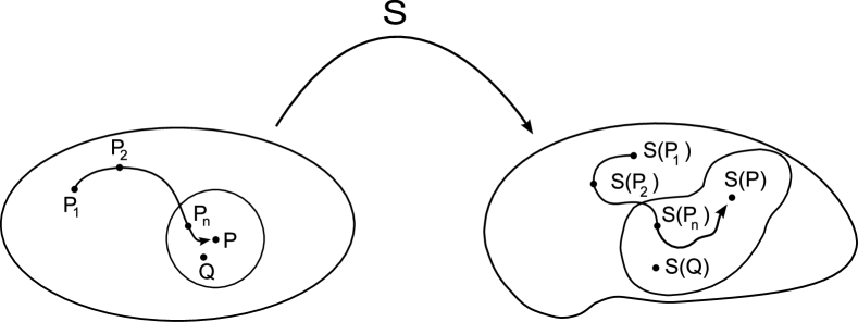
Abbildung 1: Sketch: reasoning of robustness of $S(\mathrm{P})$. Left: $\mathrm{P}$, a neighborhood of $\mathrm{P}$, and $\mathcal{M}_{1}(\mathcal{X}\times\mathcal{Y})$. Right: $S(\mathrm{P})$, a neighborhood of $S(\mathrm{P})$, and the space of all probability measures of $S(\mathrm{P})$ for $\mathrm{P}\in\mathcal{M}_{1}(\mathcal{X}\times\mathcal{Y})$.

3 Main Results

The following theorem is our main result and shows that support vector machines are qualitatively robust under mild conditions.

Theorem 3.1

Let $\mathcal{X}$ be a Polish space and let $\mathcal{Y}$ be a closed subset of $\mathds{R}$ . Let the loss function be a continuous function $\,L:\mathcal{X}\times\mathcal{Y}\times\mathds{R}\rightarrow[0,\infty)\,$ such that $L(x,y,y)=0$ for every $(x,y)\in\mathcal{X}\times\mathcal{Y}$ and

$$L(x,y,\cdot)\;:\;\;\mathds{R}\;\rightarrow\;[0,\infty)\,,\qquad t\;\mapsto\;L(x,y,t)$$

is convex for every $(x,y)\in\mathcal{X}\times\mathcal{Y}$ . Assume that the uniform Lipschitz property

$$\sup_{(x,y)\in\mathcal{X}\times\mathcal{Y}}\big{|}L(x,y,t)-L(x,y,t^{\prime})\big{|}\;\;\leq\;\;|L|_{1}\cdot|t-t^{\prime}|\qquad\;\forall\,t,t^{\prime}\in\mathds{R}$$

is fulfilled for a real number $|L|_{1}\in(0,\infty)$ . Furthermore, let $k:\mathcal{X}\times\mathcal{X}\rightarrow\mathds{R}$ be a bounded and continuous kernel with RKHS $H$ .

Then, the sequence of SVM-estimators $(S_{n})_{n\in\mathds{N}}$ is qualitatively robust.

Of course, this theorem applies to classification (e.g. $\mathcal{Y}=\{-1,1\}$) and regression (e.g. $\mathcal{Y}=\mathds{R}$ or $\mathcal{Y}=[0,\infty)$). In particular, note that every function $g:\mathcal{Y}\rightarrow\mathds{R}$ is continuous if $\mathcal{Y}$ is a discrete set – e.g. $\mathcal{Y}=\{-1,1\}$ . In this case, assuming $L$ to be continuous reduces to the assumption that

$$\mathcal{X}\times\mathds{R}\;\rightarrow\;[0,\infty)\,,\qquad(x,t)\;\mapsto\;L(x,y,t)$$

is continuous for every $y\in\mathcal{Y}$ . Many of the most common loss functions are permitted in the theorem, e.g. the hinge loss and logistic loss for classification, $\varepsilon$-insensitive loss and Huber’s loss for regression, and the pinball loss for quantile regression. The least squares loss is ruled out in Theorem 3.1 – which is not surprising as it is the prominent standard example of a loss function which typically conflicts with robustness if $\mathcal{X}$ and $\mathcal{Y}$ are unbounded; see, e.g., Christmann and Steinwart (2007) and Christmann and Van Messem (2008). Assuming continuity of the kernel $k$ does not seem to be very restrictive as all of the most common kernels are continuous. Assuming $k$ to be bounded is quite natural in order to ensure good robustness properties. While the Gaussian RBF kernel is always bounded, polynomial kernels (except for the constant kernel) and the exponential kernel are bounded if and only if $\mathcal{X}$ is bounded.

In our definition of the sequence $(S_{n})_{n\in\mathds{N}}$ of SVM-estimators, the regularization parameter $\lambda$ is a fixed real number which does not change with $n$ . Instead, it is also common to consider sequences of estimators

$$T_{n}\;:\;\;(\mathcal{X}\times\mathcal{Y})^{n}\;\rightarrow\;H\,,\qquad D_{n}\;\mapsto\;f_{L,D_{n},\lambda_{n}}\,,\qquad n\in\mathds{N}\,,$$

where the fixed parameter $\lambda$ is replaced by a sequence $(\lambda_{n})_{n\in\mathds{N}}\subset(0,\infty)$ with $\lim_{n\rightarrow\infty}\lambda_{n}=0$ . However, Theorem 3.1 cannot be generalized to $(T_{n})_{n\in\mathds{N}}$ . Proposition 5.2 (in the Appendix) shows under extremely mild conditions that $(T_{n})_{n\in\mathds{N}}$ is not qualitatively robust. This is of interest because appropriately chosen null sequences $(\lambda_{n})_{n\in\mathds{N}}\subset(0,\infty)$ are used to prove universal consistency of the risk $\,\mathcal{R}_{L^{\ast},\mathrm{P}}(f_{L^{\ast},D_{n},\lambda_{n}})\xrightarrow[]{\,\mathrm{P}}\inf_{f\in\mathcal{F}}\mathcal{R}_{L^{\ast},\mathrm{P}}(f)$  and $\,f_{L^{\ast},D_{n},\lambda_{n}}\xrightarrow[]{\,\mathrm{P}}\textup{arg}\inf_{f\in\mathcal{F}}\mathcal{R}_{L^{\ast},\mathrm{P}}(f)$  for $n\rightarrow\infty$ where $\mathcal{F}$ denotes the set of all measurable functions $f:\mathcal{X}\rightarrow\mathds{R}$. This was first shown by Steinwart (2002), Zhang (2004), and Steinwart (2005). We also refer to Bousquet and Elisseeff (2002), Bartlett et al. (2006), Christmann et al. (2009), and Steinwart and Anghel (2009).

The proof of Theorem 3.1 is based on the following result which is interesting on its own.

Theorem 3.2

Under the assumptions of Theorem 3.1, the SVM-functional

$$S\;:\;\;\mathcal{M}_{1}(\mathcal{X}\times\mathcal{Y})\;\rightarrow\;H\,,\quad\;\mathrm{P}\;\mapsto\;f_{L^{\ast},\mathrm{P},\lambda}$$

is continuous with respect to the weak topology on $\mathcal{M}_{1}(\mathcal{X}\times\mathcal{Y})$ and the norm topology on $H$ .

As a generalization of earlier results by, e.g., Zhang (2001), De Vito et al. (2004), and Steinwart (2003), Christmann et al. (2009, Theorem 7) derived a representer theorem which showed that, for every $\mathrm{P}_{0}\in\mathcal{M}_{1}(\mathcal{X}\times\mathcal{Y})$, there is a bounded map $h:\mathcal{X}\times\mathcal{Y}\rightarrow\mathds{R}$ such that $f_{L^{\ast},\mathrm{P}_{0},\lambda}=-\frac{1}{2\lambda}\int h\Phi\,d\mathrm{P}_{0}$  and

$$\big{\|}f_{L^{\ast},\mathrm{P},\lambda}-f_{L^{\ast},\mathrm{P}_{0},\lambda}\big{\|}_{H}\;\leq\;\lambda^{-1}\left\|\int h\Phi\,d\mathrm{P}-\int h\Phi\,d\mathrm{P}_{0}\right\|$$ (5)

for every $\mathrm{P}\in\mathcal{M}_{1}(\mathcal{X}\times\mathcal{Y})$ . The integrals in (5) are Bochner integrals of the vector-valued function $h\Phi:\mathcal{X}\times\mathcal{Y}\rightarrow H$ , $(x,y)\mapsto h(x,y)\Phi(x)$ where $\Phi$ is the canonical feature map of $k$ , i.e. $\Phi(x)=k(\cdot,x)$ for all $x\in\mathcal{X}$ . This offers an elegant possibility of proving Theorem 3.2 if we would accept some additional assumptions: The statement of Theorem 3.2 is true if $\int h\Phi\,d\mathrm{P}_{n}$ converges to $\int h\Phi\,d\mathrm{P}_{0}$ for every weakly convergent sequence $\mathrm{P}_{n}\rightarrow\mathrm{P}_{0}$ . In the following, we show that the integrals indeed converge – under the additional assumptions that the derivative $\frac{\partial L}{\partial t}(x,y,t)$ exists and is continuous for every $(x,y,t)\in\mathcal{X}\times\mathcal{Y}\times\mathds{R}$ . These assumptions are fulfilled e.g. for the logistic loss function and Huber’s loss function. In this case, it follows from Christmann et al. (2009, Theorem 7) that $h$ is continuous. Since $\Phi$ is continuous and bounded (see e.g. Steinwart and Christmann (2008, p. 124 and Lemma 4.29), the integrand $h\Phi:\mathcal{X}\times\mathcal{Y}\rightarrow H$ is continuous and bounded. Then, it follows from Bourbaki (2004, p. III.40) that $\int h\Phi\,d\mathrm{P}_{n}$ converges to $\int h\Phi\,d\mathrm{P}_{0}$ for every weakly convergent sequence $\mathrm{P}_{n}\rightarrow\mathrm{P}_{0}\,$ — just as in case of real-valued integrands; see Subsection 5.1 in the Appendix.

Unfortunately, this short proof only works under the additional assumption of a continuous partial derivative $\frac{\partial L}{\partial t}$ and this assumption rules out many loss functions used in practice, such as hinge, absolute distance and $\varepsilon$-insensitive for regression and pinball for quantile regression. Therefore, our proof of Theorem 3.2 (without this additional assumption) does not use the representer theorem and Bochner integrals; it is mainly based on the theory of Hilbert spaces and weak convergence of measures. In the following, we give some corollaries of Theorem 3.2.

Let $\mathcal{C}_{b}(\mathcal{X})$ be the Banach space of all bounded, continuous functions $f:\mathcal{X}\rightarrow\mathds{R}$ with norm

$$\|f\|_{\infty}\;=\;\sup_{x\in\mathcal{X}}|f(x)|\;.$$

Since $k$ is continuous and bounded, we immediately get from Theorem 3.2 and Steinwart and Christmann (2008, Lemma 4.28):

Corollary 3.3

Under the assumptions of Theorem 3.1, the SVM-functional

$$\mathcal{M}_{1}(\mathcal{X}\times\mathcal{Y})\;\rightarrow\;\mathcal{C}_{b}(\mathcal{X})\,,\quad\;\mathrm{P}\;\mapsto\;f_{L^{\ast},\mathrm{P},\lambda}$$

is continuous with respect to the weak topology on $\mathcal{M}_{1}(\mathcal{X}\times\mathcal{Y})$ and the norm topology on $\mathcal{C}_{b}(\mathcal{X})$ .

That is, $\,\sup_{x\in\mathcal{X}}\big{|}f_{L,\mathrm{P}^{\prime},\lambda}(x)-f_{L,\mathrm{P},\lambda}(x)\big{|}\,$ is small if $\mathrm{P}^{\prime}$ is close to $\mathrm{P}$ .

The next corollary is similar to Steinwart and Christmann (2008, Lemma 5.13) but only assumes continuity instead of differentiability of $t\mapsto L(x,y,t)$. In combination with existence and uniqueness of support vector machines (see Theorem 2.1), this result shows that a support vector machine is the solution of a well-posed mathematical problem in the sense of Hadamard (1902).

Corollary 3.4

Under the assumptions of Theorem 3.1, the SVM-estimator

$$S_{n}\;:\;\;(\mathcal{X}\times\mathcal{Y})^{n}\;\rightarrow\;H\,,\qquad D_{n}\;\mapsto\;f_{L,D_{n},\lambda}$$

is continuous.

In particular, it follows from Corollary 3.4 that the SVM-estimator $S_{n}$ is measurable.

Remark 3.5

Let $d_{n}$ be a metric which generates the topology on $(\mathcal{X}\times\mathcal{Y})^{n}$ , e.g. the Euclidean metric on $\mathds{R}^{n(k+1)}$ if $\mathcal{X}\subset\mathds{R}^{k}$ . Then Corollary 3.4 and Steinwart and Christmann (2008, Lemma 4.28) imply the following continuity property of the SVM-estimator: For every $\varepsilon>0$ and every data set $D_{n}\in(\mathcal{X}\times\mathcal{Y})^{n}$, there is a $\delta>0$ such that

$$\sup_{x\in\mathcal{X}}\big{|}f_{L,D_{n}^{\prime},\lambda}(x)-f_{L,D_{n},\lambda}(x)\big{|}\;<\;\varepsilon$$

if $D_{n}^{\prime}\in(\mathcal{X}\times\mathcal{Y})^{n}$ is any other data set with $n$ observations and $\,d_{n}(D_{n}^{\prime},D_{n})<\delta$.

We finish this section with a corollary about strong consistency of support vector machines which arises as a by-product of Theorem 3.2. Often, asymptotic results of support vector machines show the convergence in probability of the risk $\mathcal{R}_{L^{\ast},\mathrm{P}}(f_{L^{\ast},\mathds{D}_{n},\lambda_{n}})$ to the Bayes risk $\inf_{f\in\mathcal{F}}\mathcal{R}_{L^{\ast},\mathrm{P}}(f)$ and of $f_{L^{\ast},\mathds{D}_{n},\lambda_{n}}$ to $\textup{arg}\inf_{f\in\mathcal{F}}\mathcal{R}_{L^{\ast},\mathrm{P}}(f)$ , where $\mathcal{F}$ is the set of all measurable functions $f:\mathcal{X}\rightarrow\mathds{R}$ and $(\lambda_{n})_{n\in\mathds{N}}$ is a suitable null sequence. In contrast to that, the following corollary provides for fixed $\lambda\in(0,\infty)$ almost sure convergence of $\mathcal{R}_{L^{\ast},\mathrm{P}}(f_{L^{\ast},\mathds{D}_{n},\lambda})$ to $\mathcal{R}_{L^{\ast},\mathrm{P}}(f_{L^{\ast},\mathrm{P},\lambda})$ and of $f_{L^{\ast},\mathds{D}_{n},\lambda}$ to $f_{L^{\ast},\mathrm{P},\lambda}$ . This is an interesting fact, although the limit $\mathcal{R}_{L^{\ast},\mathrm{P}}(f_{L^{\ast},\mathrm{P},\lambda})$ will in general differ from the Bayes risk.

Recall from Section 2 that the data points $(x_{i},y_{i})$ from the data set $D_{n}=\big{(}(x_{1},x_{2}),\dots(x_{n},y_{n})\big{)}$ are realizations of i.i.d. random variables

$$(X_{i},Y_{i})\;:\;\;(\Omega,{\cal A},\mathrm{Q})\;\longrightarrow\;\big{(}\mathcal{X}\times\mathcal{Y},\mathfrak{B}(\mathcal{X}\times\mathcal{Y})\big{)}\;,\qquad n\in\mathds{N}\,,$$

such that

$$(X_{i},Y_{i})\;\sim\;\mathrm{P}\qquad\quad\forall\,n\in\mathds{N}\;.$$

Corollary 3.6

Define the random vectors

$$\mathds{D}_{n}\;:=\;\big{(}(X_{1},Y_{1}),\dots,(X_{n},Y_{n})\big{)}$$

and the corresponding $H$-valued random functions

$$f_{L^{\ast},\mathds{D}_{n},\lambda}\;=\;\textup{arg}\inf_{f\in H}\,\frac{1}{n}\sum_{i=1}^{n}L^{\ast}\big{(}X_{i},Y_{i},f(X_{i})\big{)}\,+\,\lambda\|f\|_{H}^{2}\;,\qquad n\in\mathds{N}\,.$$

From the assumptions of Theorem 3.1, it follows that

(a) ${\displaystyle\;\lim_{n\rightarrow\infty}\|f_{L^{\ast},\mathds{D}_{n},\lambda}-f_{L^{\ast},\mathrm{P},\lambda}\|_{H}\;=\;0\qquad\text{almost sure}}$

(b) ${\displaystyle\;\lim_{n\rightarrow\infty}\,\sup_{x\in\mathcal{X}}|f_{L^{\ast},\mathds{D}_{n},\lambda}(x)-f_{L^{\ast},\mathrm{P},\lambda}(x)|\;=\;0\qquad\text{almost sure}}$

(c) ${\displaystyle\;\lim_{n\rightarrow\infty}\,\mathcal{R}_{L^{\ast},\mathrm{P},\lambda}(f_{L^{\ast},\mathds{D}_{n},\lambda})\;=\;\mathcal{R}_{L^{\ast},\mathrm{P},\lambda}(f_{L^{\ast},\mathrm{P},\lambda})\qquad\text{almost sure}}$

(d) ${\displaystyle\;\lim_{n\rightarrow\infty}\,\mathcal{R}_{L^{\ast},\mathrm{P}}(f_{L^{\ast},\mathds{D}_{n},\lambda})\;=\;\mathcal{R}_{L^{\ast},\mathrm{P}}(f_{L^{\ast},\mathrm{P},\lambda})\qquad\text{almost sure.}}$

If the support vector machine $f_{L,\mathrm{P},\lambda}$ exists, then assertions (a)–(d) are also valid for $L$ instead of $L^{\ast}$ .

4 Conclusions

It is well-known that outliers in data sets or other moderate model violations can pose a serious problem to a statistical analysis. On the one hand, practitioners can hardly guarantee that their data sets do not contain any outliers, while, on the other hand, many statistical methods are very sensitive even to small violations of the assumed statistical model. Since support vector machines play an important role in statistical machine learning, investigating their performance in the presence of moderate model violations is a crucial topic – the more so as support vector machines are frequently applied to large and complex high-dimensional data sets.

In this article, we showed that support vector machines are qualitatively robust with a fixed regularization parameter $\lambda\in(0,\infty)$, i.e., the performance of support vector machines is hardly affected by the following two kinds of errors: large errors in a small fraction of the data set and small errors in the whole data set. This not only means that these errors do not lead to large errors in the support vector machines but also that even the finite sample distribution of support vector machines is hardly affected.

In contrast to that, we also showed that support vector machines are not qualitatively robust any more under extremely mild conditions, if the fixed regularization parameter $\lambda$ is replaced by a sequence of parameters $\lambda_{n}\in(0,\infty)$ which decreases to 0 with increasing sample size $n$. From our point of view, this is an important result as all universal consistency proofs we know of for support vector machines or for their risks, use an appropriate null sequence $\lambda_{n}\in(0,\infty)$, $n\in\mathds{N}$.

5 Appendix

In Subsection 5.1, we briefly recall some facts about weak convergence of probability measures. In addition, we show that weak convergence of probability measures on a Polish space implies convergence of the corresponding Bochner integrals of bounded, continuous functions. Subsection 5.2 demonstrates under extremely mild conditions that the sequence of SVM-estimators cannot be qualitatively robust if the fixed regularization parameter $\lambda$ is replaced by a sequence $(\lambda_{n})_{n\in\mathds{N}}\subset(0,\infty)$ with $\lim_{n\rightarrow\infty}\lambda_{n}=0$ . Subsection 5.3 contains all proofs.

5.1 Weak Convergence of Probability Measures and Bochner Integrals

Let $\mathcal{Z}$ be a Polish space with Borel-$\sigma$-algebra $\mathfrak{B}(\mathcal{Z})$, let $d$ be a metric on $\mathcal{Z}$ which generates the topology on $\mathcal{Z}$ and let $\mathcal{M}_{1}(\mathcal{Z})$ be the set of all probability measures on $(\mathcal{Z},\mathfrak{B}(\mathcal{Z}))$ .

A sequence $(\mathrm{P}_{n})_{n\in\mathds{N}}$ of probability measures on $\mathcal{Z}$ converges to a probability measure $\mathrm{P}_{0}$ in the weak topology on $\mathcal{M}_{1}(\mathcal{Z})$ if

$$\lim_{n\rightarrow\infty}\int g\,d\mathrm{P}_{n}\;=\;\int g\,d\mathrm{P}_{0}\qquad\forall\,g\in\mathcal{C}_{b}(\mathcal{Z})$$

where $\mathcal{C}_{b}(\mathcal{Z})$ denotes the set of all bounded, continuous functions $g:\mathcal{Z}\rightarrow\mathds{R}$ , see Billingsley (1968, § 1).

The weak topology on $\mathcal{M}_{1}(\mathcal{Z})$ is metrizable by the Prokhorov metric $d_{\textrm{Pro}}$ ; see e.g. Huber (1981, § 2.2). The Prokhorov metric $d_{\textrm{Pro}}$ on $\mathcal{M}_{1}(\mathcal{Z})$ is defined by

$$d_{\textrm{Pro}}(\mathrm{P}_{1},\mathrm{P}_{2})\;=\;\inf\big{\{}\varepsilon\in(0,\infty)\;\big{|}\;\;\mathrm{P}_{1}(B)\,<\,\mathrm{P}_{2}(B^{\varepsilon})+\varepsilon\;\;\forall\,B\in\mathfrak{B}(\mathcal{Z})\big{\}}$$

where $B^{\varepsilon}=\{z\in\mathcal{Z}\,|\,\inf_{z^{\prime}\in\mathcal{Z}}d(z,z^{\prime})<\varepsilon\}$ .

Let $g:\mathcal{Z}\rightarrow\mathds{R}$ be a continuous and bounded function. By definition, we have $\lim_{n\rightarrow\infty}\int g\,d\mathrm{P}_{n}=\int g\,d\mathrm{P}_{0}$ for every sequence $(\mathrm{P}_{n})_{n\in\mathds{N}}\subset\mathcal{M}_{1}(\mathcal{Z})$ which converges weakly in $\mathcal{M}_{1}(\mathcal{Z})$ to some $\mathrm{P}_{0}$ . The following theorem states that this is still valid for Bochner integrals if $g$ is replaced by a vector-valued continuous and bounded function $\Psi:\mathcal{Z}\rightarrow H$ , where $H$ is a separable Banach space. This follows from a corresponding statement in Bourbaki (2004, p. III.40) for locally compact spaces $\mathcal{Z}$. Boundedness of $\Psi$ means that $\sup_{z\in\mathcal{Z}}\|\Psi(z)\|_{H}<\infty$ .

Theorem 5.1

Let $\mathcal{Z}$ be a Polish space with Borel-$\sigma$-algebra $\mathfrak{B}(\mathcal{Z})$ and let $H$ be a separable Banach space. If $\Psi:\mathcal{Z}\rightarrow H$ is a continuous and bounded function, then

$$\int\Psi\,d\mathrm{P}_{n}\;\;\longrightarrow\;\;\int\Psi\,d\mathrm{P}_{0}\qquad(n\rightarrow\infty)$$

for every sequence $(\mathrm{P}_{n})_{n\in\mathds{N}}\subset\mathcal{M}_{1}(\mathcal{Z})$ which converges weakly in $\mathcal{M}_{1}(\mathcal{Z})$ to some $\mathrm{P}_{0}$ .

5.2 A Counterexample

Theorem 3.1 shows that, for a fixed regularization parameter $\lambda\in(0,\infty)$ , the sequence of SVM-estimators

$$S_{n}\;:\;\;(\mathcal{X}\times\mathcal{Y})^{n}\;\rightarrow\;H\,,\qquad D_{n}\;\mapsto\;f_{L,D_{n},\lambda}\,,\qquad n\in\mathds{N}\,,$$

is qualitatively robust. The following proposition shows that, under extremely mild conditions, the sequence of estimators

$$T_{n}\;:\;\;(\mathcal{X}\times\mathcal{Y})^{n}\;\rightarrow\;H\,,\qquad D_{n}\;\mapsto\;f_{L,D_{n},\lambda_{n}}\,,\qquad n\in\mathds{N}\,,$$

cannot be qualitatively robust if the fixed parameter $\lambda$ is replaced by a sequence $(\lambda_{n})_{n\in\mathds{N}}\subset(0,\infty)$ with $\lim_{n\rightarrow\infty}\lambda_{n}=0$ . This shows that the asymptotic results on universal consistency of support vector machines – which consider appropriate null sequences $(\lambda_{n})_{n\in\mathds{N}}\subset(0,\infty)$ – are in conflict with qualitative robustness of support vector machines using $\lambda_{n}$ . (Asymptotic results on universal consistency of support vector machines can be found, e.g., in the references listed before Theorem 3.2.)

For simplicity, the following proposition focuses on regression because it is assumed that $\{0,1\}\subset\mathcal{Y}$ . A similar proposition (with a similar proof) can also be given in case of binary classification where $\mathcal{Y}=\{-1,1\}$ .

Proposition 5.2

Let $\mathcal{X}$ be a Polish space and let $\mathcal{Y}$ be a closed subset of $\mathds{R}$ such that $\{0,1\}\subset\mathcal{Y}$ . Let $k$ be a bounded kernel with RKHS $H$ . Let $L$ be a convex loss function such that $L(x,y,y)=0$ for every $(x,y)\in\mathcal{X}\times\mathcal{Y}$ . In addition, assume that there are $x_{0},x_{1}\in\mathcal{X}$ such that

$$\exists\,\tilde{f}\in H\,:\quad\tilde{f}(x_{0})=0\,,\quad\tilde{f}(x_{1})\not=0$$ (6)

$$L(x_{1},1,0)\;>\;0\;.$$ (7)

Let $(\lambda_{n})_{n\in\mathds{N}}\subset(0,\infty)$ be any sequence such that $\lim_{n\rightarrow\infty}\lambda_{n}=0$ . Then, the sequence of estimators

$$T_{n}\;:\;\;(\mathcal{X}\times\mathcal{Y})^{n}\;\rightarrow\;H\,,\qquad D_{n}\;\mapsto\;f_{L,D_{n},\lambda_{n}}\,,\qquad n\in\mathds{N}\,,$$

is not qualitatively robust.

5.3 Proofs

In order to prove the main theorem, i.e. Theorem 3.1, we have to prove Theorem 3.2 and Corollary 3.4 at first.

Proof of Theorem 3.2: Since the proof is somewhat involved, we start with a short outline. The proof is divided into four parts. Part 1 is concerned with some important preparations. We have to show that $(f_{L^{\ast},\mathrm{P}_{n},\lambda})_{n\in\mathds{N}}$ converges to $f_{L^{\ast},\mathrm{P}_{0},\lambda}$ in $H$ if the sequence of probability measures $(\mathrm{P}_{n})_{n\in\mathds{N}}$ weakly converges to the probability measure $\mathrm{P}_{0}$ . Let us now assume that there is a subsequence $(f_{L^{\ast},\mathrm{P}_{n_{\ell}},\lambda})_{\ell\in\mathds{N}}$ of $(f_{L^{\ast},\mathrm{P}_{n},\lambda})_{n\in\mathds{N}}$ which weakly converges to $f_{L^{\ast},\mathrm{P}_{0},\lambda}$ in $H$ . Then, it is shown in Part 2 and Part 3 that

$$\lim_{\ell\rightarrow\infty}\mathcal{R}_{L^{\ast},\mathrm{P}_{n_{\ell}}}(f_{L^{\ast},\mathrm{P}_{n_{\ell}},\lambda}) = \mathcal{R}_{L^{\ast},\mathrm{P}_{0}}(f_{L^{\ast},\mathrm{P}_{0},\lambda})$$ (8)

$$\lim_{\ell\rightarrow\infty}\mathcal{R}_{L^{\ast},\mathrm{P}_{n_{\ell}},\lambda}(f_{L^{\ast},\mathrm{P}_{n_{\ell}},\lambda}) = \mathcal{R}_{L^{\ast},\mathrm{P}_{0},\lambda}(f_{L^{\ast},\mathrm{P}_{0},\lambda})\;\;.$$ (9)

Because of

$$\|f\|_{H}^{2}\;=\;\frac{1}{\lambda}\Big{(}\mathcal{R}_{L^{\ast},\mathrm{P},\lambda}(f)-\mathcal{R}_{L^{\ast},\mathrm{P}}(f)\Big{)}\qquad\,\forall\,\mathrm{P}\in\mathcal{M}_{1}(\mathcal{X}\times\mathcal{Y})\quad\forall\,f\in H\;,$$

it follows from (8) and (9) that $\lim_{\ell\rightarrow\infty}\|f_{L^{\ast},\mathrm{P}_{n_{\ell}},\lambda}\|_{H}=\|f_{L^{\ast},\mathrm{P}_{0},\lambda}\|_{H}$ . Since this convergence of the norms together with weak convergence in the Hilbert space $H$ implies (strong) convergence in $H$, we get that the subsequence $(f_{L^{\ast},\mathrm{P}_{n_{\ell}},\lambda})_{\ell\in\mathds{N}}$ converges to $f_{L^{\ast},\mathrm{P}_{0},\lambda}$ in $H$ . Part 4 extends this result to the whole sequence $(f_{L^{\ast},\mathrm{P}_{n},\lambda})_{n\in\mathds{N}}$ . The main difficulty in the proof is the verification of (8) in Part 3.

In order to shorten notation, define

$$L_{f}^{\ast}:\;\,\mathcal{X}\times\mathcal{Y}\;\rightarrow\;\mathds{R}\,,\quad\;(x,y)\;\mapsto\;L^{\ast}\big{(}x,y,f(x)\big{)}=L(x,y,f(x))-L(x,y,0)$$

for every measurable $f:\mathcal{X}\rightarrow\mathds{R}$ . Following e.g. van der Vaart (1998) and Pollard (2002), we use the notation

$$\mathrm{P}g\;=\;\int g\,d\mathrm{P}$$

for integrals of real-valued functions $g$ with respect to $\mathrm{P}$ . This leads to a very efficient notation which is more intuitive here because, in the following, $\mathrm{P}$ rather acts as a linear functional on a function space than as a probability measure on a $\sigma$-algebra.

By use of these notations, we may write

$$\mathrm{P}L^{\ast}_{f}\;=\;\int L_{f}^{\ast}\,d\mathrm{P}\;=\;\mathcal{R}_{L^{\ast},\mathrm{P}}(f)$$

for the (shifted) risk of $f\in H$ . Accordingly, the (shifted) regularized risk of $f\in H$ is

$$\mathcal{R}_{L^{\ast},\mathrm{P},\lambda}(f)\;=\;\mathcal{R}_{L^{\ast},\mathrm{P}}(f)\,+\,\lambda\|f\|_{H}^{2}\;=\;\mathrm{P}L^{\ast}_{f}\,+\,\lambda\|f\|_{H}^{2}\;.$$

Part 1: Since the loss function $L$ , the shifted loss $L^{\ast}$ and the regularization parameter $\lambda\in(0,\infty)$ are fixed, we may drop them in the notation and write

$$f_{\mathrm{P}}\;:=\;f_{L^{\ast},\mathrm{P},\lambda}\;=\;S(\mathrm{P})\qquad\forall\,\mathrm{P}\in\mathcal{M}_{1}(\mathcal{X}\times\mathcal{Y})\;.$$

Recall from Theorem 2.1 that $f_{L^{\ast},\mathrm{P},\lambda}$ is equal to the support vector machine $f_{L,\mathrm{P},\lambda}$ if $f_{L,\mathrm{P},\lambda}$ exists. That is, we have $f_{\mathrm{P}}=f_{L,\mathrm{P},\lambda}$ in the latter case. According to Christmann et al. (2009, (17),(16)),

$$\|f_{\mathrm{P}}\|_{\infty} \leq \frac{1}{\lambda}|L|_{1}\cdot\|k\|_{\infty}^{2}$$ (10)

$$\|f_{\mathrm{P}}\|_{H} \leq \sqrt{\frac{1}{\lambda}|L|_{1}\int|f_{\mathrm{P}}|\,d\mathrm{P}\,}\;\stackrel{{\scriptstyle(\ref{theorem-continuity-of-svm-functional-1})}}{{\leq}}\;\frac{1}{\lambda}|L|_{1}\cdot\|k\|_{\infty}\;.\qquad$$ (11)

for every $\mathrm{P}\in\mathcal{M}_{1}(\mathcal{X}\times\mathcal{Y})$ . Since the kernel $k$ is continuous and bounded, Steinwart and Christmann (2008, Lemma 4.28) yields

$$f\;\in\;\mathcal{C}_{b}(\mathcal{X})\qquad\forall\,f\in H\;.$$ (12)

Therefore, continuity of $L$ implies continuity of

$$L_{f}^{\ast}\;:\;\;\mathcal{X}\times\mathcal{Y}\;\rightarrow\;\mathds{R}\,,\qquad(x,y)\;\mapsto\;L\big{(}x,y,f(x)\big{)}-L(x,y,0)$$

for every $f\in H$ . Furthermore, the uniform Lipschitz property of $L$ implies

$$\sup_{x,y}\big{|}L_{f}^{\ast}(x,y)\big{|}\;=\;\sup_{x,y}\big{|}L(x,y,f(x))-L(x,y,0)\big{|}$$

$$\leq \sup_{x^{\prime},x,y}\big{|}L(x,y,f(x^{\prime}))-L(x,y,0)\big{|}\;\leq\;\sup_{x^{\prime}}|L|_{1}\cdot\big{|}f(x^{\prime})-0\big{|}\;=\;|L|_{1}\|f\|_{\infty}$$

for every $f\in H$ . Hence, we obtain

$$L_{f}^{\ast}\;\in\;\mathcal{C}_{b}(\mathcal{X}\times\mathcal{Y})\qquad\forall\,f\in H\;.$$ (13)

In particular, the above calculation and (10) imply

$$\|L_{f_{\mathrm{P}}}^{\ast}\|_{\infty}\;\leq\;\frac{1}{\lambda}|L|_{1}^{2}\cdot\|k\|_{\infty}^{2}\quad\;\forall\,\mathrm{P}\in\mathcal{M}_{1}(\mathcal{X}\times\mathcal{Y})\;.$$ (14)

For the remaining parts of the proof, let $\,(\mathrm{P}_{n})_{n\in\mathds{N}_{0}}\subset\mathcal{M}_{1}(\mathcal{X}\times\mathcal{Y})$  be any fixed sequence such that

$$\mathrm{P}_{n}\;\longrightarrow\;\mathrm{P}_{0}\qquad(n\rightarrow\infty)$$

in the weak topology on $\mathcal{M}_{1}(\mathcal{X}\times\mathcal{Y})$ – that is,

$$\lim_{n\rightarrow\infty}\mathrm{P}_{n}g\;=\;\mathrm{P}_{0}g\qquad\forall\,g\in\mathcal{C}_{b}(\mathcal{X}\times\mathcal{Y})\;.$$ (15)

In particular, (13) and (15) imply

$$\lim_{n\rightarrow\infty}\mathrm{P}_{n}L_{f}^{\ast}\;=\;\mathrm{P}_{0}L_{f}^{\ast}\qquad\forall\,f\in H\;.$$ (16)

In order to shorten the notation, define

$$f_{n}\;:=\;f_{\mathrm{P}_{n}}\,=\,f_{L^{\ast},\mathrm{P}_{n},\lambda}\,=\,S(\mathrm{P}_{n})\qquad\forall\,n\in\mathds{N}\cup\{0\}\;.$$

Hence, we have to show that $(f_{n})_{n\in\mathds{N}}$ converges to $f_{0}$ in $H$ – that is,

$$\lim_{n\rightarrow\infty}\|f_{n}-f_{0}\|_{H}\;=\;0\;.$$ (17)

Part 2: In this part of the proof, it is shown that

$$\limsup_{n\rightarrow\infty}\,\mathrm{P}_{n}L^{\ast}_{f_{n}}+\lambda\|f_{n}\|^{2}_{H}\;\leq\;\mathrm{P}_{0}L^{\ast}_{f_{0}}+\lambda\|f_{0}\|^{2}_{H}\;.$$ (18)

Due to (13), the mapping

$$\mathcal{M}_{1}(\mathcal{X}\times\mathcal{Y})\;\rightarrow\;\mathds{R}\,,\qquad\mathrm{P}\;\mapsto\;\mathrm{P}L^{\ast}_{f}+\lambda\|f\|^{2}_{H}$$

is defined well and continuous for every $f\in H$ . As being the (pointwise) infimum over a family of continuous functions, the function

$$\mathcal{M}_{1}(\mathcal{X}\times\mathcal{Y})\;\rightarrow\;\mathds{R}\,,\qquad\mathrm{P}\;\mapsto\;\inf_{f\in H}\,\big{(}\mathrm{P}L^{\ast}_{f}+\lambda\|f\|^{2}_{H}\big{)}$$

is upper semicontinuous; see, e.g., Denkowski et al. (2003, Prop. 1.1.36). Therefore, the definition of $f_{n}$ implies

$$\limsup_{n\rightarrow\infty}\,\big{(}\mathrm{P}_{n}L^{\ast}_{f_{n}}+\lambda\|f_{n}\|^{2}_{H}\big{)}\;=\;\limsup_{n\rightarrow\infty}\,\inf_{f\in H}\,\big{(}\mathrm{P}_{n}L^{\ast}_{f}+\lambda\|f\|^{2}_{H}\big{)}\;\leq$$

$$\leq\;\inf_{f\in H}\,\big{(}\mathrm{P}_{0}L^{\ast}_{f}+\lambda\|f\|^{2}_{H}\big{)}\;=\;\mathrm{P}_{0}L^{\ast}_{f_{0}}+\lambda\|f_{0}\|^{2}_{H}\;\;.\qquad\qquad\qquad$$

Part 3: In this part of the proof, the following statement is shown:

Let $(f_{n_{\ell}})_{\ell\in\mathds{N}}$ be a subsequence of $(f_{n})_{n\in\mathds{N}}$ and assume that $(f_{n_{\ell}})_{\ell\in\mathds{N}}$ converges weakly in $H$ to some $f_{0}^{\prime}\in H$. Then, the following three assertions are true:

$$\lim_{\ell\rightarrow\infty}\mathrm{P}_{n_{\ell}}L^{\ast}_{f_{n_{\ell}}}\;=\;\mathrm{P}_{0}L^{\ast}_{f_{0}^{\prime}}\qquad$$ (19)

$$\qquad\quad f_{0}^{\prime}\;=\;f_{0}\qquad$$ (20)

$$\lim_{\ell\rightarrow\infty}\|f_{n_{\ell}}-f_{0}\|_{H}\;=\;0\;\;.\quad$$ (21)

In order to prove this, we will also have to deal with subsequences of the subsequence $(f_{n_{\ell}})_{\ell\in\mathds{N}}$ . As this would lead to a somewhat cumbersome notation, we define

$$\mathrm{P}^{\prime}_{\ell}\;:=\;\mathrm{P}_{n_{\ell}}\quad\text{and}\quad f^{\prime}_{\ell}\;:=\;f_{n_{\ell}}\qquad\ell\in\mathds{N}\;.$$

Thus, $f^{\prime}_{\ell}=f_{L^{\ast},\mathrm{P}_{n_{\ell}},\lambda}$ for every $\ell\in\mathds{N}$ . Then, the assumption of weak convergence in the Hilbert space $H$ equals

$$\lim_{\ell\rightarrow\infty}\langle f^{\prime}_{\ell},h\rangle_{H}\;\;=\;\;\langle f^{\prime}_{0},h\rangle_{H}\qquad\forall\,h\in H\;.$$ (22)

First of all, we show (19) by proving

$$\limsup_{\ell\rightarrow\infty}\big{|}\mathrm{P}_{\ell}^{\prime}L^{\ast}_{f_{\ell}^{\prime}}-\mathrm{P}_{0}L^{\ast}_{f_{0}^{\prime}}\big{|}\;\leq\;\varepsilon_{0}$$ (23)

for every fixed $\varepsilon_{0}>0$. In order to do this, fix any $\varepsilon_{0}>0$ and define

$$\varepsilon\;:=\;\frac{\varepsilon_{0}}{\,|L|_{1}\cdot\big{(}{\textstyle\frac{1}{\lambda}}|L|_{1}\cdot\|k\|_{\infty}^{2}+\|f_{0}^{\prime}\|_{\infty}\big{)}}\;\;>\;\;0\;.$$ (24)

The following calculation shows that the sequence of functions $(f_{\ell}^{\prime})_{\ell\in\mathds{N}}$ is uniformly continuous on $\mathcal{X}$ . For any convergent sequence $x_{m}\rightarrow x_{0}$ in $\mathcal{X}$ , we have

$$\limsup_{m\rightarrow\infty}\sup_{\ell\in\mathds{N}}\,\big{|}f_{\ell}^{\prime}(x_{m})-f_{\ell}^{\prime}(x_{0})\big{|}$$

$$\;\;=\;\limsup_{m\rightarrow\infty}\,\sup_{\ell\in\mathds{N}}\,\big{|}\langle f_{\ell}^{\prime},\Phi(x_{m})\rangle_{H}-\langle f_{\ell}^{\prime},\Phi(x_{0})\rangle_{H}\big{|}$$

$$\;\;=\;\limsup_{m\rightarrow\infty}\,\sup_{\ell\in\mathds{N}}\,\big{|}\langle f_{\ell}^{\prime},\Phi(x_{m})-\Phi(x_{0})\rangle_{H}\big{|}$$

$$\;\;\leq\;\limsup_{m\rightarrow\infty}\,\sup_{\ell\in\mathds{N}}\,\|f_{\ell}^{\prime}\|_{H}\cdot\|\Phi(x_{m})-\Phi(x_{0})\|_{H}$$

$$\;\stackrel{{\scriptstyle(\ref{theorem-continuity-of-svm-functional-2})}}{{\leq}}\;\frac{1}{\lambda}\,|L|_{1}\cdot\|k\|_{\infty}\cdot\limsup_{m\rightarrow\infty}\,\|\Phi(x_{m})-\Phi(x_{0})\|_{H}\;=\;0\qquad\quad$$

where the first equality follows from the properties of the RKHS $H$ and the last equality follows from Steinwart and Christmann (2008, Lemma 4.29).

Since $\mathcal{X}\times\mathcal{Y}$ is a Polish space, weak convergence of $(\mathrm{P}_{\ell}^{\prime})_{\ell\in\mathds{N}}$ implies uniform tightness of $(\mathrm{P}_{\ell}^{\prime})_{\ell\in\mathds{N}}$ (see e.g. Dudley (1989, Theorem 11.5.3)). That is, there is a compact subset $K_{\varepsilon}\subset\mathcal{X}\times\mathcal{Y}$ such that

$$\limsup_{\ell\rightarrow\infty}\,\mathrm{P}_{\ell}^{\prime}\big{(}K_{\varepsilon}^{\,\textup{c}}\big{)}\;<\;\varepsilon\;.$$ (25)

Since $K_{\varepsilon}$ is compact and the projection

$$\tau_{\mathcal{X}}:\;\;\mathcal{X}\times\mathcal{Y}\;\rightarrow\;\mathcal{X}\,,\qquad(x,y)\;\mapsto\;x$$

is continuous, $\,\tilde{K}_{\varepsilon}:=\tau_{X}(K_{\varepsilon})\,$ is compact in $\mathcal{X}$ . For every $\ell\in\mathds{N}_{0}$ , the restriction of $f_{\ell}^{\prime}$ on $\tilde{K}_{\varepsilon}$ is denoted by $\tilde{f}_{\ell}^{\prime}$ . As the sequence $(f_{\ell}^{\prime})_{\ell\in\mathds{N}}$ is uniformly continuous on $\mathcal{X}$ and uniformly bounded in $\mathcal{C}_{b}(\mathcal{X})$ (see (10)), the sequence of the restrictions $(\tilde{f}_{\ell}^{\prime})_{\ell\in\mathds{N}}$ has the corresponding properties on $\tilde{K}_{\varepsilon}$ . That is, $(\tilde{f}_{\ell}^{\prime})_{\ell\in\mathds{N}}$ is uniformly continuous on $\tilde{K}_{\varepsilon}$ and uniformly bounded in $\mathcal{C}_{b}(\tilde{K}_{\varepsilon})$ . Hence, the Arzela-Ascoli-Theorem – see Conway (1985, Theorem VI.3.8) – assures that $(\tilde{f}_{\ell}^{\prime})_{\ell\in\mathds{N}}$ is totally bounded and, therefore, relatively compact in $\mathcal{C}_{b}(\tilde{K}_{\varepsilon})$ (since $\mathcal{C}_{b}(\tilde{K}_{\varepsilon})$ is a complete metric space); see e.g. Dunford and Schwartz (1958, Theorem I.6.15).

The following reasoning shows that $(\tilde{f}_{\ell}^{\prime})_{\ell\in\mathds{N}}$ converges to $\tilde{f}_{0}^{\prime}$ in $\mathcal{C}_{b}(\tilde{K}_{\varepsilon})$ , i.e.

$$\lim_{\ell\rightarrow\infty}\;\sup_{x\in\tilde{K}_{\varepsilon}}\big{|}f_{\ell}^{\prime}(x)-f_{0}^{\prime}(x)\big{|}\;=\;0\;.$$ (26)

We will show (26) by contradiction. If (26) is not true, then there is a $\delta>0$ and a subsequence $(\tilde{f}_{\ell_{j}}^{\prime})_{j\in\mathds{N}}$ such that

$$\sup_{x\in\tilde{K}_{\varepsilon}}\big{|}f_{\ell_{j}}^{\prime}(x)-f_{0}^{\prime}(x)\big{|}\;>\;\delta\qquad\forall\,j\in\mathds{N}\;.$$ (27)

Relative compactness of $(\tilde{f}_{\ell}^{\prime})_{\ell\in\mathds{N}}$ implies that there is a further subsequence $(\tilde{f}_{\ell_{j_{m}}}^{\prime})_{m\in\mathds{N}}$ which converges in $\mathcal{C}_{b}(\tilde{K}_{\varepsilon})$ to some $\tilde{h}_{0}\in\mathcal{C}_{b}(\tilde{K}_{\varepsilon})$ . Then,

$$\tilde{h}_{0}(x) = \lim_{m\rightarrow\infty}\tilde{f}_{\ell_{j_{m}}}^{\prime}(x)\;=\;\lim_{m\rightarrow\infty}f_{\ell_{j_{m}}}^{\prime}(x)\;=\;\lim_{m\rightarrow\infty}\langle f_{\ell_{j_{m}}}^{\prime},\Phi(x)\rangle_{H}\;=$$

$$\stackrel{{\scriptstyle(\ref{theorem-continuity-of-svm-functional-11})}}{{=}} \langle f_{0}^{\prime},\Phi(x)\rangle_{H}\;=\;f_{0}^{\prime}(x)\;=\;\tilde{f}_{0}^{\prime}(x)\;\;.$$

for every $x\in\tilde{K}_{\varepsilon}$ . That is, $\tilde{f}_{0}^{\prime}$ is the limit of $(\tilde{f}_{\ell_{j_{m}}}^{\prime})_{m\in\mathds{N}}$ – which is the desired contradiction to (27). Therefore, (26) is true.

Now, we can prove (23): Firstly, the triangle inequality and the Lipschitz continuity of $L$ yield

$$\limsup_{\ell\rightarrow\infty}\big{|}\mathrm{P}_{\ell}^{\prime}L^{\ast}_{f_{\ell}^{\prime}}-\mathrm{P}_{0}L^{\ast}_{f_{0}^{\prime}}\big{|}\;\leq\;\limsup_{\ell\rightarrow\infty}\,\,\big{|}\mathrm{P}_{\ell}^{\prime}L^{\ast}_{f_{\ell}^{\prime}}-\mathrm{P}_{\ell}^{\prime}L^{\ast}_{f_{0}^{\prime}}\big{|}+\big{|}\mathrm{P}_{\ell}^{\prime}L^{\ast}_{f_{0}^{\prime}}-\mathrm{P}_{0}L^{\ast}_{f_{0}^{\prime}}\big{|}$$

$$\stackrel{{\scriptstyle(\ref{theorem-continuity-of-svm-functional-6a})}}{{=}} \limsup_{\ell\rightarrow\infty}\big{|}\mathrm{P}_{\ell}^{\prime}L^{\ast}_{f_{\ell}^{\prime}}-\mathrm{P}_{\ell}^{\prime}L^{\ast}_{f_{0}^{\prime}}\big{|}$$

$$= \limsup_{\ell\rightarrow\infty}\left|\int\!L(x,y,f_{\ell}^{\prime}(x))-L(x,y,f_{0}^{\prime}(x))\,\,d\mathrm{P}_{\ell}^{\prime}\right|$$

$$\leq \limsup_{\ell\rightarrow\infty}\int|L|_{1}\cdot\big{|}f_{\ell}^{\prime}(x)-f_{0}^{\prime}(x)\big{|}\,\,\mathrm{P}_{\ell}^{\prime}(d(x,y))\;=$$

$$= |L|_{1}\cdot\limsup_{\ell\rightarrow\infty}\,\,\Bigg{(}\int_{K_{\varepsilon}}\big{|}f_{\ell}^{\prime}(x)-f_{0}^{\prime}(x)\big{|}\,\,\mathrm{P}_{\ell}^{\prime}(d(x,y))\,+$$

$$\qquad\qquad\qquad\qquad\qquad+\;\int_{K_{\varepsilon}^{\textup{c}}}\big{|}f_{\ell}^{\prime}(x)-f_{0}^{\prime}(x)\big{|}\,\,\mathrm{P}_{\ell}^{\prime}(d(x,y))\Bigg{)}\;\;\;.\quad\quad$$

Secondly, using $\,\tilde{K}_{\varepsilon}=\tau_{X}(K_{\varepsilon})\,$, we obtain

$$\limsup_{\ell\rightarrow\infty}\,\,\int_{K_{\varepsilon}}\big{|}f_{\ell}^{\prime}(x)-f_{0}^{\prime}(x)\big{|}\,\,\mathrm{P}_{\ell}^{\prime}(d(x,y))$$

$$\leq \limsup_{\ell\rightarrow\infty}\,\sup_{(x,y)\in K_{\varepsilon}}\big{|}f_{\ell}^{\prime}(x)-f_{0}^{\prime}(x)\big{|}\,=\,\limsup_{\ell\rightarrow\infty}\,\sup_{x\in\tilde{K}_{\varepsilon}}\big{|}f_{\ell}^{\prime}(x)-f_{0}^{\prime}(x)\big{|}\;\stackrel{{\scriptstyle(\ref{theorem-continuity-of-svm-functional-15})}}{{=}}\;0\,.$$

Thirdly,

$$\limsup_{\ell\rightarrow\infty}\,\,\int_{K_{\varepsilon}^{\textup{c}}}\big{|}f_{\ell}^{\prime}(x)-f_{0}^{\prime}(x)\big{|}\,\,\mathrm{P}_{\ell}^{\prime}(d(x,y))$$

$$\leq \limsup_{\ell\rightarrow\infty}\,\,\mathrm{P}_{\ell}^{\prime}\big{(}K_{\varepsilon}^{\textup{c}}\big{)}\cdot\big{(}\|f_{\ell}^{\prime}\|_{\infty}+\|f_{0}^{\prime}\|_{\infty}\big{)}$$

$$\stackrel{{\scriptstyle(\ref{theorem-continuity-of-svm-functional-14})}}{{\leq}} \limsup_{\ell\rightarrow\infty}\,\,\varepsilon\cdot\big{(}\|f_{\ell}^{\prime}\|_{\infty}+\|f_{0}^{\prime}\|_{\infty}\big{)}\;\;\stackrel{{\scriptstyle(\ref{theorem-continuity-of-svm-functional-1}),(\ref{theorem-continuity-of-svm-functional-13})}}{{=}}\;\;\frac{\varepsilon_{0}}{\,|L|_{1}}\;\;\;.$$

Combining these three calculations proves (23). Since $\varepsilon_{0}>0$ was arbitrarily chosen in (23), this proves (19).

Next, we prove (20): Due to weak convergence of $(f_{n_{\ell}})_{\ell\in\mathds{N}}$ in $H$, it follows from Conway (1985, Exercise V.1.9) that

$$\|f_{0}^{\prime}\|_{H}\;\leq\;\liminf_{\ell\rightarrow\infty}\|f_{n_{\ell}}\|_{H}\;.$$ (28)

Therefore, the definition of $f_{0}=f_{L^{\ast},\mathrm{P}_{0},\lambda}$ implies

$$\mathrm{P}_{0}L^{\ast}_{f_{0}}+\lambda\|f_{0}\|^{2}_{H}\;=\;\inf_{f\in H}\,\mathrm{P}_{0}L^{\ast}_{f}+\lambda\|f\|^{2}_{H}$$

$$\leq \mathrm{P}_{0}L^{\ast}_{f_{0}^{\prime}}+\lambda\|f_{0}^{\prime}\|^{2}_{H}\;\stackrel{{\scriptstyle(\ref{theorem-continuity-of-svm-functional-8}),(\ref{theorem-continuity-of-svm-functional-16})}}{{\leq}}\;\liminf_{\ell\rightarrow\infty}\,\mathrm{P}_{n_{\ell}}L^{\ast}_{f_{n_{\ell}}}+\lambda\|f_{n_{\ell}}\|^{2}_{H}$$

$$\leq \limsup_{\ell\rightarrow\infty}\,\mathrm{P}_{n_{\ell}}L^{\ast}_{f_{n_{\ell}}}+\lambda\|f_{n_{\ell}}\|^{2}_{H}\;\stackrel{{\scriptstyle(\ref{theorem-continuity-of-svm-functional-7a})}}{{\leq}}\;\mathrm{P}_{0}L^{\ast}_{f_{0}}+\lambda\|f_{0}\|^{2}_{H}\;\;.$$

Due to this calculation, it follows that

$$\mathrm{P}_{0}L^{\ast}_{f_{0}}+\lambda\|f_{0}\|^{2}_{H}\;=\;\inf_{f\in H}\,\mathrm{P}_{0}L^{\ast}_{f}+\lambda\|f\|^{2}_{H}\;=\;\mathrm{P}_{0}L^{\ast}_{f_{0}^{\prime}}+\lambda\|f_{0}^{\prime}\|^{2}_{H}$$ (29)

and

$$\mathrm{P}_{0}L^{\ast}_{f_{0}}+\lambda\|f_{0}\|^{2}_{H}\;=\;\lim_{\ell\rightarrow\infty}\,\mathrm{P}_{n_{\ell}}L^{\ast}_{f_{n_{\ell}}}+\lambda\|f_{n_{\ell}}\|^{2}_{H}\;.$$ (30)

According to Theorem 2.1, $f_{0}=f_{L^{\ast},\mathrm{P}_{0},\lambda}$ is the unique minimizer of the function

$$H\;\rightarrow\;\mathds{R}\,,\quad f\;\mapsto\;\mathrm{P}_{0}L^{\ast}_{f}+\lambda\|f\|^{2}_{H}$$

and, therefore, (29) implies $f_{0}=f_{0}^{\prime}$  –  i.e. (20).

Completing Part 3 of the proof, (21) is shown now:

$$\lim_{\ell\rightarrow\infty}\|f_{n_{\ell}}\|_{H}^{2} = \lim_{\ell\rightarrow\infty}\,\frac{1}{\lambda}\Big{(}\big{(}\mathrm{P}_{n_{\ell}}L^{\ast}_{f_{n_{\ell}}}+\lambda\|f_{n_{\ell}}\|^{2}_{H}\big{)}\,\,-\,\,\mathrm{P}_{n_{\ell}}L^{\ast}_{f_{n_{\ell}}}\Big{)}$$

$$\stackrel{{\scriptstyle(\ref{theorem-continuity-of-svm-functional-8}),(\ref{theorem-continuity-of-svm-functional-18})}}{{=}} \,\frac{1}{\lambda}\Big{(}\big{(}\mathrm{P}_{0}L^{\ast}_{f_{0}}+\lambda\|f_{0}\|^{2}_{H}\big{)}\,\,-\,\,\mathrm{P}_{0}L^{\ast}_{f_{0}}\Big{)}\;=\;\|f_{0}\|_{H}^{2}\;\;.$$

By assumption, the sequence $(f_{n_{\ell}})_{\ell\in\mathds{N}}$ converges weakly to some $f_{0}^{\prime}\in H$ and by (20), we know that $f_{0}^{\prime}=f_{0}$. In addition, we have proven $\lim_{\ell\rightarrow\infty}\|f_{n_{\ell}}\|_{H}=\|f_{0}\|_{H}$ now. This convergence of the norms together with weak convergence implies strong convergence in the Hilbert space $H$, – see, e.g., Conway (1985, Exercise V.1.8). That is, we have proven (21).

Part 4: In this final part of the proof, (17) is shown. This is done by contradiction: If (17) is not true, there is an $\varepsilon>0$ and a subsequence $(f_{n_{\ell}})_{\ell\in\mathds{N}}$ of $(f_{n})_{n\in\mathds{N}}$ such that

$$\|f_{n_{\ell}}-f_{0}\|_{H}\;>\;\varepsilon\qquad\forall\,\ell\in\mathds{N}$$ (31)

According to (11) , $(f_{n_{\ell}})_{\ell\in\mathds{N}}=(f_{\mathrm{P}_{n_{\ell}}})_{\ell\in\mathds{N}}$ is bounded in $H$ . Hence, the sequence $(f_{n_{\ell}})_{\ell\in\mathds{N}}$ contains a further subsequence that weakly converges in $H$ to some $f_{0}^{\prime}$ ; see e.g. Dunford and Schwartz (1958, Corollary IV.4.7). Without loss of generality, we may therefore assume that $(f_{n_{\ell}})_{\ell\in\mathds{N}}$ weakly converges in $H$ to some $f_{0}^{\prime}$ . (Otherwise, we can choose another subsequence in (31)). Next, it follows from Part 3, that $(f_{n_{\ell}})_{\ell\in\mathds{N}}$ strongly converges in $H$ to $f_{0}$ – which is a contradiction to (31). $\Box$

Proof of Corollary 3.4: Let $(D_{n,m})_{m\in\mathds{N}}$ be a sequence in $(\mathcal{X}\times\mathcal{Y})^{n}$ which converges to some $D_{n,0}\in(\mathcal{X}\times\mathcal{Y})^{n}$ . Then, the corresponding sequence of empirical measures $\big{(}\mathds{P}_{D_{n,m}}\big{)}_{m\in\mathds{N}}$ weakly converges in $\mathcal{M}_{1}(\mathcal{X}\times\mathcal{Y})$ to $\mathds{P}_{D_{n,0}}$ . Therefore, the statement follows from Theorem 3.2 and (4). $\Box$

Based on Cuevas (1988), the main theorem essentially is a consequence of Theorem 3.2.

Proof of Theorem 3.1: According to Corollary 3.4, the SVM-estimator

$$S_{n}\;:\;\;(\mathcal{X}\times\mathcal{Y})^{n}\;\rightarrow\;H\,,\qquad D_{n}\;\mapsto\;f_{L,D_{n},\lambda}$$

is continuous and, therefore, measurable with respect to the Borel-$\sigma$-algebras for every $n\in\mathds{N}$ . The mapping

$$S\;:\;\;\mathcal{M}_{1}(\mathcal{X}\times\mathcal{Y})\;\rightarrow\;H\,,\quad\;\mathrm{P}\;\mapsto\;f_{L^{\ast},\mathrm{P},\lambda}$$

is a continuous functional due to Theorem 3.2. Furthermore,

$$S_{n}(D_{n})\;=\;S\big{(}\mathds{P}_{D_{n}}\big{)}\qquad\forall\,D_{n}\in(\mathcal{X}\times\mathcal{Y})^{n}\qquad\quad\forall\,n\in\mathds{N}\;.$$

As already mentioned in Section 2, $H$ is a separable Hilbert space and, therefore, a Polish space. Hence, the sequence of SVM-estimators $(S_{n})_{n\in\mathds{N}}$ is qualitatively robust according to Cuevas (1988, Theorem 2). $\Box$

Proof of Corollary 3.6: Let $\mathds{P}_{\mathds{D}_{n}}$ denote the function which maps $\omega\in\Omega$ to the empirical measure $\frac{1}{n}\sum_{i=1}^{n}\delta_{(X_{i}(\omega),Y_{i}(\omega))}$ . According to Varadarajan’s Theorem (Dudley (1989, Theorem 11.4.1)), there is a set $N\in\mathcal{A}$ such that $\mathrm{Q}(N)=0$ and $\mathds{P}_{\mathds{D}_{n}(\omega)}$ weakly converges to $\mathrm{P}$ for every $\omega\in\Omega\setminus N$ . Then, Theorem 3.2 implies

$$\lim_{n\rightarrow\infty}\|f_{L^{\ast},\mathds{D}_{n}(\omega),\lambda}-f_{L^{\ast},\mathrm{P},\lambda}\|_{H}\;\stackrel{{\scriptstyle(\ref{representation-of-empirical-svm})}}{{=}}\;\lim_{n\rightarrow\infty}\|S(\mathds{P}_{\mathds{D}_{n}(\omega)})-S(\mathrm{P})\|_{H}\;=\;0$$

for every $\omega\in\Omega\setminus N$ . This proves (a) and, due to Steinwart and Christmann (2008, Lemma 4.28), (b). The Lipschitz continuity of $L^{\ast}$ implies

$$\big{|}\mathcal{R}_{L^{\ast},\mathrm{P}}(f_{L^{\ast},\mathds{D}_{n}(\omega),\lambda})-\mathcal{R}_{L^{\ast},\mathrm{P}}(f_{L^{\ast},\mathrm{P},\lambda})\big{|}$$

$$=\;\left|\int L(x,y,f_{L^{\ast},\mathds{D}_{n}(\omega),\lambda}(x))-L(x,y,f_{L^{\ast},\mathrm{P},\lambda}(x))\,\mathrm{P}(d(x,y))\right|$$

$$\leq\;\int\sup_{x^{\prime},y^{\prime}}\big{|}L(x^{\prime},y^{\prime},f_{L^{\ast},\mathds{D}_{n}(\omega),\lambda}(x))-L(x^{\prime},y^{\prime},f_{L^{\ast},\mathrm{P},\lambda}(x))\big{|}\,\mathrm{P}(d(x,y))$$

$$\leq\;\int|L|_{1}\cdot\big{|}f_{L^{\ast},\mathds{D}_{n}(\omega),\lambda}(x)-f_{L^{\ast},\mathrm{P},\lambda}(x)\big{|}\,\mathrm{P}(d(x,y))$$

$$\leq\;|L|_{1}\cdot\big{\|}f_{L^{\ast},\mathds{D}_{n}(\omega),\lambda}-f_{L^{\ast},\mathrm{P},\lambda}\big{\|}_{\infty}$$

for every $\omega\in\Omega$ . According to (b), the last term converges to 0 for $\mathrm{Q}$ - almost every $\omega\in\Omega$ and this implies (d). Finally, (c) follows from (a) and (d).

If $f_{L,\mathrm{P},\lambda}$ exists, then $f_{L^{\ast},\mathrm{P},\lambda}$ is equal to $f_{L,\mathrm{P},\lambda}$ (Theorem 2.1). In particular, there is an $f\in H$ such that $(x,y)\mapsto L(x,y,f(x))$ is $\mathrm{P}$ - integrable. Since Lipschitz-continuity of $L$ and $H\subset\mathcal{C}_{b}(\mathcal{X})$ (see Steinwart and Christmann (2008, Lemma 4.28)) implies $\mathrm{P}$ - integrability of $(x,y)\mapsto L^{\ast}(x,y,f(x))=L(x,y,f(x))-L(x,y,0)$ , we get that $(x,y)\mapsto L(x,y,0)$ is also $\mathrm{P}$ - integrable. Therefore, $\mathcal{R}_{L^{\ast},\mathrm{P}}(f)$ is equal to $\mathcal{R}_{L,\mathrm{P}}(f)-\mathcal{R}_{L,\mathrm{P}}(0)$ for every $f\in H$, and $\mathcal{R}_{L,\mathrm{P}}(0)$ is a finite constant which does not depend on $f$ . Furthermore, $f_{L^{\ast},D_{n},\lambda}=f_{L,D_{n},\lambda}$ for every $D_{n}\in(\mathcal{X}\times\mathcal{Y})^{n}$ ; see Section 2. Hence, the original assertions (a)–(d) for $L^{\ast}$ turn into the corresponding assertions for $L$ instead of $L^{\ast}$ . $\Box$

Proof of Theorem 5.1: If $\Psi=0$ , the statement is true. Assume $\Psi\not=0$ now and assume that the statement of the theorem is not true. Then, there is an $\varepsilon>0$ and a subsequence $(\mathrm{P}_{n_{\ell}})_{\ell\in\mathds{N}}$ such that

$$\bigg{\|}\int\Psi\,d\mathrm{P}_{n_{l}}-\int\Psi\,d\mathrm{P}_{0}\bigg{\|}_{H}\;>\;\varepsilon\qquad\forall\,\ell\in\mathds{N}\;.$$ (32)

Since the sequence $(\mathrm{P}_{n})_{n\in\mathds{N}}$ weakly converges to $\mathrm{P}_{0}$, it is uniformly tight; see, e.g., (Dudley, 1989, Theorem 11.5.3). That is, there is a compact subset $K\subset\mathcal{Z}$ such that

$$\mathrm{P}_{n_{\ell}}\big{(}\mathcal{Z}\setminus K\big{)}\;<\;\frac{\varepsilon}{4\sup_{z}\|\Psi(z)\|_{H}}\qquad\forall\,\ell\in\mathds{N}_{0}\;.$$ (33)

For every $\ell\in\mathds{N}$ , let $\tilde{\mathrm{P}}_{n_{\ell}}$ denote the restriction of $\mathrm{P}_{n_{\ell}}$ to the Borel-$\sigma$-algebra $\mathfrak{B}(K)$ of $K$ . Let $\tilde{\Psi}$ denote the restriction of $\Psi$ to $K$. Since $K$ is a compact Polish space, the set $\mathcal{M}(K)$ of all finite signed measures on $\mathfrak{B}(K)$ is the dual space of $\mathcal{C}(K)$ (the set of all continuous functions $f:K\rightarrow\mathds{R}$); see e.g. (Dudley, 1989, Theorem 7.1.1 and 7.4.1). Accordingly, $\mathcal{M}(K)$ is precisely the set of all (real) measures in the sense of (Bourbaki, 2004, Section III.1); see also (Bourbaki, 2004, Subsection III.1.5 and III.1.8). Since $(\tilde{\mathrm{P}}_{n_{\ell}})_{\ell\in\mathds{N}}$ is relatively compact in the vague topology of $\mathcal{M}(K)$ (Bourbaki, 2004, Subsection III.1.9), we may assume without loss of generality that $(\tilde{\mathrm{P}}_{n_{\ell}})_{\ell\in\mathds{N}}$ vaguely converges to some positive finite measure $\tilde{\mathrm{P}}_{0}^{\prime}$. (Otherwise, we may replace $(\tilde{\mathrm{P}}_{n_{\ell}})_{\ell\in\mathds{N}}$ by a further subsequence.) According to (Bourbaki, 2004, p. III.40), vague convergence implies

$$\int\tilde{\Psi}\,d\tilde{\mathrm{P}}_{n_{\ell}}\;\;\longrightarrow\;\;\int\tilde{\Psi}\,d\tilde{\mathrm{P}}_{0}^{\prime}\qquad(\ell\rightarrow\infty)$$ (34)

for Pettis and Bochner integrals (since $H$ is assumed to be a separable Banach space, Pettis integrals and Bochner integrals coincide; see e.g. (Dudley, 1989, p. 150)).

Let $H^{\ast}$ be the dual space of $H$. Note that $F\circ\Psi$ is continuous and bounded on $\mathcal{Z}$ for every $F\in H^{\ast}$. Hence, it follows from weak convergence of $(\mathrm{P}_{n_{\ell}})_{\ell\in\mathds{N}}$ to $\mathrm{P}_{0}$ and a property of the Bochner integral (Denkowski et al., 2003, Theorem 3.10.16) that

$$\lim_{\ell\rightarrow\infty}F\bigg{(}\int\Psi\,d\mathrm{P}_{n_{\ell}}\bigg{)}=\lim_{\ell\rightarrow\infty}\int F\circ\Psi\,d\mathrm{P}_{n_{\ell}}=\int F\circ\Psi\,d\mathrm{P}_{0}=F\bigg{(}\int\Psi\,d\mathrm{P}_{0}\bigg{)}.$$

Accordingly, vague convergence of $(\tilde{\mathrm{P}}_{n_{\ell}})_{\ell\in\mathds{N}}$ to $\tilde{\mathrm{P}}_{0}^{\prime}$ implies $\lim_{\ell\rightarrow\infty}F\big{(}\int\tilde{\Psi}\,d\tilde{\mathrm{P}}_{n_{\ell}}\big{)}=F\big{(}\int\tilde{\Psi}\,d\tilde{\mathrm{P}}_{0}^{\prime}\big{)}$. Hence,

$$\lim_{\ell\rightarrow\infty}F\bigg{(}\int\Psi\,d\mathrm{P}_{n_{\ell}}-\int\tilde{\Psi}\,d\tilde{\mathrm{P}}_{n_{\ell}}\bigg{)}\;=\;F\bigg{(}\int\Psi\,d\mathrm{P}_{0}-\int\tilde{\Psi}\,d\tilde{\mathrm{P}}_{0}^{\prime}\bigg{)}\;.$$ (35)

For every $\ell\in\mathds{N}$,

$$\bigg{\|}\int\!\!\Psi\,d\mathrm{P}_{n_{\ell}}-\!\!\int\!\!\tilde{\Psi}\,d\tilde{\mathrm{P}}_{n_{\ell}}\bigg{\|}_{H}=\bigg{\|}\int_{\mathcal{Z}\setminus K}\!\Psi\,d\mathrm{P}_{n_{\ell}}\bigg{\|}_{H}\leq\int_{\mathcal{Z}\setminus K}\|\Psi\|_{H}\,d\mathrm{P}_{n_{\ell}}\stackrel{{\scriptstyle(\ref{theorem-continuity-bochner-1})}}{{\leq}}\frac{\varepsilon}{4}\,.\;$$ (36)

For every $\ell\in\mathds{N}$ and every $F\in H^{\ast}$ such that $\|F\|_{H^{\ast}}\leq 1$, (36) implies $\big{|}F\big{(}\int\Psi\,d\mathrm{P}_{n_{\ell}}-\int\tilde{\Psi}\,d\tilde{\mathrm{P}}_{n_{\ell}}\big{)}\big{|}\,\leq\,\frac{\varepsilon}{4}$ and, because of (35), also $\big{|}F\big{(}\int\Psi\,d\mathrm{P}_{n_{\ell}}-\int\tilde{\Psi}\,d\tilde{\mathrm{P}}_{n_{\ell}}\big{)}\big{|}\,\leq\,\frac{\varepsilon}{4}$ . Hence, it follows from (Dunford and Schwartz, 1958, Corollary II.3.15) that

$$\bigg{\|}\int\Psi\,d\mathrm{P}_{0}-\int\tilde{\Psi}\,d\tilde{\mathrm{P}}_{0}^{\prime}\bigg{\|}_{H}\;\leq\;\frac{\varepsilon}{4}\;.$$ (37)

By using the triangle inequality, we obtain

$$\bigg{\|}\int\Psi\,d\mathrm{P}_{n_{\ell}}-\int\Psi\,d\mathrm{P}_{0}\bigg{\|}_{H}$$

$$\leq \!\!\!\bigg{\|}\!\int\!\!\Psi\,d\mathrm{P}_{n_{\ell}}\!-\!\!\int\!\!\tilde{\Psi}\,d\tilde{\mathrm{P}}_{n_{\ell}}\bigg{\|}_{H}\!\!+\bigg{\|}\int\!\!\tilde{\Psi}\,d\tilde{\mathrm{P}}_{n_{\ell}}\!-\!\!\int\!\!\tilde{\Psi}\,d\tilde{\mathrm{P}}_{0}^{\prime}\bigg{\|}_{H}\!\!+\bigg{\|}\int\!\!\tilde{\Psi}\,d\tilde{\mathrm{P}}_{0}^{\prime}\!-\!\!\int\!\!\Psi\,d\mathrm{P}_{0}\bigg{\|}_{H}\!,$$

so that (34), (36) and (37) imply $\limsup_{\ell\rightarrow\infty}\left\|\int\Psi\,d\mathrm{P}_{n_{\ell}}-\int\Psi\,d\mathrm{P}_{0}\right\|_{H}\,\leq\,\frac{\varepsilon}{2}.$ This is a contradiction to (32). $\Box$

Proof of Proposition 5.2: Without loss of generality, we may assume that

$$\tilde{f}(x_{0})=0\qquad\text{and}\qquad\tilde{f}(x_{1})=1\;.$$ (38)

(Otherwise, we can divide $\tilde{f}$ by $\tilde{f}(x_{1})$ .) Since the function $\mathds{R}\rightarrow[0,\infty),\;\;t\mapsto L(x_{1},1,t)$ is convex, it is also continuous. Therefore, (7) implies the existence of an $\gamma\in(0,1)$ such that

$$L(x_{1},1,\gamma)\;>\;0\;.$$ (39)

Note that convexity of the loss function, $L(x_{1},1,1)=0$ and $L(x_{1},1,\gamma)>0$ imply

$$0\;=\;L(x_{1},1,1)\;\leq\;L(x_{1},1,t)\;<\;L(x_{1},1,\gamma)\;\leq\;L(x_{1},1,s)$$ (40)

for $0\leq s\leq\gamma<t\leq 1$ . Define $\mathrm{P}_{0}:=\delta_{(x_{0},0)}$ . Since $f_{L,\delta_{(x_{0},0)},\lambda_{n}}\,=\,0$ , it follows that

$$\mathrm{P}_{0}^{n}\Big{(}\big{\{}D_{n}\in(\mathcal{X}\times\mathcal{Y})^{n}\;\big{|}\;\;f_{L,D_{n},\lambda_{n}}\,=\,0\big{\}}\Big{)}\;\;=\;\;1\;.$$ (41)

Next, fix any $\varepsilon\in(0,1)$ and define the mixture distribution

$$\mathrm{P}_{\varepsilon}\;:=\;(1-\varepsilon)\mathrm{P}_{0}+\varepsilon\delta_{(x_{1},1)}\;=\;(1-\varepsilon)\delta_{(x_{0},0)}+\varepsilon\delta_{(x_{1},1)}\;.$$

For every $n\in\mathds{N}$ , let $\mathcal{Z}_{n}^{\prime}$ be the subset of $(\mathcal{X}\times\mathcal{Y})^{n}$ which consists of all those elements $D_{n}=\big{(}D_{n}^{(1)},\dots,D_{n}^{(n)}\big{)}\in(\mathcal{X}\times\mathcal{Y})^{n}$ where

$$D_{n}^{(i)}\,\in\,\big{\{}(x_{0},0),(x_{1},1)\big{\}}\qquad\forall\,i\in\{1,\dots,n\}\;.$$

In addition, let $\mathcal{Z}_{n}^{\prime\prime}$ be the subset of $(\mathcal{X}\times\mathcal{Y})^{n}$ which consists of all those elements $D_{n}=\big{(}D_{n}^{(1)},\dots,D_{n}^{(n)}\big{)}\in(\mathcal{X}\times\mathcal{Y})^{n}$ where

$$\sharp\,\Big{(}\!\big{\{}i\in\{1,\dots,n\}\;\big{|}\;\;D_{n}^{(i)}=(x_{1},1)\big{\}}\!\Big{)}\;\geq\;\frac{\varepsilon}{2}\;.$$ (42)

Define $\mathcal{Z}_{n}:=\mathcal{Z}_{n}^{\prime}\cap\mathcal{Z}_{n}^{\prime\prime}$ . Then, we have $\mathrm{P}_{\varepsilon}^{n}(\mathcal{Z}_{n}^{\prime})=1$ and, according to the law of large numbers (Dudley (1989, Theorem 8.3.5)), $\lim_{n\rightarrow\infty}\mathrm{P}^{n}_{\varepsilon}(\mathcal{Z}_{n}^{\prime\prime})=1$ . Hence, there is an $n_{\varepsilon,1}\in\mathds{N}$ such that

$$\mathrm{P}^{n}_{\varepsilon}(\mathcal{Z}_{n})\;\geq\;\frac{1}{2}\qquad\forall\,n\geq n_{\varepsilon,1}\;.$$ (43)

Due to $\lim_{n\rightarrow\infty}\lambda_{n}=0$ and (39), there is an $n_{\varepsilon,2}\in\mathds{N}$ such that

$$\lambda_{n}\|\tilde{f}\|_{H}^{2}\;<\;\frac{\varepsilon}{2}L(x_{1},1,\gamma)\qquad\forall\,n\geq n_{\varepsilon,2}\;.$$ (44)

In the following, we show

$$f_{L,D_{n},\lambda_{n}}(x_{1})\;>\;\gamma\qquad\forall\,D_{n}\in\mathcal{Z}_{n}\,,\quad\forall\,n\geq n_{\varepsilon,2}\;.$$ (45)

To this end, fix any $D_{n}\in\mathcal{Z}_{n}$ . In order to prove (45), it is enough to show the following assertion for every $n\geq n_{\varepsilon,2}$ :

$$\;\;f\in H\,,\;\;f(x_{1})\leq\gamma\quad\;\Rightarrow\;\quad\mathcal{R}_{L,D_{n},\lambda_{n}}(\tilde{f})\;\leq\;\mathcal{R}_{L,D_{n},\lambda_{n}}(f)\;.$$ (46)

The definition of $\mathcal{Z}_{n}$ and (38) imply

$$\mathcal{R}_{L,D_{n},\lambda_{n}}(\tilde{f})\;=\;\mathcal{R}_{L,D_{n}}(\tilde{f})\,+\,\lambda_{n}\|\tilde{f}\|_{H}^{2}\;=\;\lambda_{n}\|\tilde{f}\|_{H}^{2}\;\;.$$

For every $f\in H$ such that $f(x_{1})\leq\gamma$, the definition of $\mathcal{Z}_{n}$ implies

$$\mathcal{R}_{L,D_{n},\lambda_{n}}(f)\;\geq\;\mathcal{R}_{L,D_{n}}(f)\;\stackrel{{\scriptstyle(\ref{prop-counterexample-102})}}{{\geq}}\;\frac{\varepsilon}{2}L\big{(}x_{1},1,f(x_{1})\big{)}\;\stackrel{{\scriptstyle(\ref{prop-counterexample-1})}}{{\geq}}\;\frac{\varepsilon}{2}L\big{(}x_{1},1,f(x_{1})\big{)}\;.$$

Hence, (46) follows from (44) and, therefore, we have proven (45).

Define $n_{\varepsilon}=\max\{n_{\varepsilon,1},n_{\varepsilon,2}\}$ . By assumption, $k$ is a bounded, non-zero kernel. According to Steinwart and Christmann (2008, Lemma 4.23), this implies

$$\|f_{L,D_{n},\lambda_{n}}\|_{H}\;\geq\;\frac{\,\|f_{L,D_{n},\lambda_{n}}\|_{\infty}}{\|k\|_{\infty}}\;\stackrel{{\scriptstyle(\ref{prop-counterexample-5})}}{{\geq}}\;\frac{\gamma}{\|k\|_{\infty}}\qquad\forall\,D_{n}\in\mathcal{Z}_{n}\,,\quad\forall\,n\geq n_{\varepsilon}$$

and, therefore,

$$\qquad\|f_{L,D_{n},\lambda_{n}}\|_{H}\;\geq\;\min\left\{\frac{\gamma}{\|k\|_{\infty}}\,,\,1\right\}\;=:\;c\quad\;\;\forall\,D_{n}\in\mathcal{Z}_{n}\,,\;\;\forall\,n\geq n_{\varepsilon}\,.$$ (47)

Define $F:=\{f\in H\,|\,\,\|f\|_{H}\geq c\}\,$ and

$$\qquad F^{\frac{c}{2}}:=\big{\{}f\in H\,\big{|}\,\,\inf_{f^{\prime}\in H}\|f-f^{\prime}\|_{H}\leq{\textstyle\frac{c}{2}}\big{\}}\;\subset\;\big{\{}f\in H\,\big{|}\;\|f\|_{H}>0\big{\}}\;.$$ (48)

Hence, for every $n\geq n_{\varepsilon}$ , we obtain

$$\big{[}T_{n}(\mathrm{P}_{\varepsilon}^{n})\big{]}(F)\;=\;\mathrm{P}_{\varepsilon}^{n}\Big{(}\big{\{}D_{n}\,\big{|}\,\|f_{L,D_{n},\lambda_{n}}\|_{H}\geq c\big{\}}\Big{)}\;\stackrel{{\scriptstyle(\ref{prop-counterexample-6})}}{{\geq}}\;\mathrm{P}_{\varepsilon}^{n}(\mathcal{Z}_{n})$$

$$\stackrel{{\scriptstyle(\ref{prop-counterexample-3})}}{{\geq}}\;\frac{1}{2}\;\stackrel{{\scriptstyle(\ref{prop-counterexample-6})}}{{\geq}}\;\frac{\,c}{\,2}\;\stackrel{{\scriptstyle(\ref{prop-counterexample-2})}}{{=}}\;\mathrm{P}_{0}^{n}\Big{(}\big{\{}D_{n}\,\big{|}\,\|f_{L,D_{n},\lambda_{n}}\|_{H}>0\big{\}}\Big{)}\,+\,\frac{\,c}{\,2}\qquad$$

$$=\;\big{[}T_{n}(\mathrm{P}_{0}^{n})\big{]}\Big{(}\big{\{}f\in H\;\big{|}\;\|f\|_{H}>0\big{\}}\Big{)}\,+\,\frac{\,c}{\,2}$$

$$\stackrel{{\scriptstyle(\ref{prop-counterexample-7})}}{{\geq}}\;\big{[}T_{n}(\mathrm{P}_{0}^{n})\big{]}\Big{(}F^{\frac{c}{2}}\Big{)}\,+\,\frac{\,c}{\,2}\;.$$

According to the definition of the Prokhorov distance (see Subsection 5.1), it follows that

$$\sup_{n\in\mathds{N}}\,d_{\textrm{Pro}}\Big{(}T_{n}(\mathrm{P}_{0}^{n}),T_{n}(\mathrm{P}_{\varepsilon}^{n})\Big{)}\;\geq\;\frac{\,c}{\,2}$$ (49)

In addition, we have $d_{\textrm{Pro}}\big{(}\mathrm{P}_{0},\mathrm{P}_{\varepsilon}\big{)}\leq\varepsilon$ because $\mathrm{P}_{\varepsilon}$ is an $\varepsilon$-mixture of $\mathrm{P}_{0}$ . Since $c>0$ does not depend on $\varepsilon\in(0,1)$ and $\varepsilon$ may be arbitrarily small, this proves that $(T_{n})_{n\in\mathds{N}}$ is not qualitatively robust in $\mathrm{P}_{0}$ . $\Box$