Spectral properties of higher order
anharmonic oscillators

Abstract.

We discuss spectral properties of the self-adjoint operator

$$-\frac{d^{2}}{dt^{2}}+\Bigl{(}\frac{t^{k+1}}{k+1}-\alpha\Bigr{)}^{2}$$

in $L^{2}(\mathbb{R})$ for odd integers $k$. We prove that the minimum over $\alpha$ of the ground state energy of this operator is attained at a unique point which tends to zero as $k$ tends to infinity. Moreover, we show that the minimum is non-degenerate. These questions arise naturally in the spectral analysis of Schrödinger operators with magnetic field. This extends or clarifies previous results by Pan-Kwek [11], Helffer-Morame [8], Aramaki [1], Helffer-Kordyukov [4, 6, 7] and Helffer [3].

1. Introduction

1.1. Definition of $\mathfrak{Q}^{(k)}(\alpha)$ and main result

For any $\alpha\in\mathbb{R}$ we denote by $\lambda_{1,\mathfrak{Q}^{(k)}(\alpha)}$ the lowest eigenvalue of the self-adjoint second order differential operator

$$\mathfrak{Q}^{(k)}(\alpha)=-\frac{d^{2}}{dt^{2}}+\Bigl{(}\frac{t^{k+1}}{k+1}-\alpha\Bigr{)}^{2}.$$

We also denote by $\mathfrak{q}^{(k)}(\alpha)$ the quadratic form corresponding to $\mathfrak{Q}^{(k)}(\alpha)$,

$$\mathfrak{q}^{(k)}(\alpha)[u]=\int_{\mathbb{R}}\bigl{|}u^{\prime}(t)|^{2}+\Bigl{(}\frac{t^{k+1}}{k+1}-\alpha\Bigr{)}^{2}|u(t)|^{2}\,\mathrm{d}t.$$

The main result of the present paper is the following theorem.

Theorem 1.1.

Assume that $k\geq 1$ is an odd integer. There exists a unique $\alpha_{\text{min}}^{(k)}$ such that

$$\inf_{\alpha\in\mathbb{R}}\lambda_{1,\mathfrak{Q}^{(k)}(\alpha)}=\lambda_{1,\mathfrak{Q}^{(k)}(\alpha_{\text{min}}^{(k)})}.$$ (1.1)

Moreover, $\alpha_{\text{min}}^{(k)}>0$ and the minimum is non-degenerate,

$$\partial^{2}_{\alpha\alpha}\bigl{(}\lambda_{1,\mathfrak{Q}^{(k)}(\alpha)}\bigr{)}\bigm{|}_{\alpha=\alpha_{\text{min}}^{(k)}}>0.$$ (1.2)

Theorem 1.2.

Assume that $k$ is even. Then $\alpha=0$ is a non-degenerate local minimum of $\lambda_{1,\mathfrak{Q}^{(k)}(\alpha)}$.

Theorem 1.3.

If $k$ is odd,

$$\lim_{k\to+\infty}\alpha_{\text{min}}^{(k)}=0.$$ (1.3)

In the even case, there exists $k_{0}$ such that for $k\geq k_{0}$ ($k$ even), the ground state energy $\lambda_{1,\mathfrak{Q}^{(k)}(\alpha)}$ has a unique minimum which is attained at $\alpha=0$.

1.2. Historical context

The operator $\mathfrak{Q}^{(k)}(\alpha)$ was first introduced in the context of magnetic Schrödinger operators in [10], and was further studied in [8, 11, 4].

The uniqueness of $\alpha_{min}^{(k)}$ was first observed numerically in [10] for $k=1$. A proof for $k=1$ was given in [11], which was completed in [3]. The uniqueness for $k>1$ ($k$ odd) was announced in [1] but the given proof seems incomplete. The non-degeneracy was obtained for $k=1$ in [3] and conjectured in the general case in [6] and [7]. This conjecture was supported by numerical computations performed by V. Bonnaillie-Noël, see Table 1. The results for large $k$ were announced in [6] and a proof was sketched in [5].

Table 1. Numerical values calculated by V. Bonnaillie-Noël with an accuracy of $10^{-2}$.

$k$	1	2	3	4	5	6	7	8	9	10
$\alpha_{\text{min}}^{(k)}$	0.35	0	0.16	0	0.10	0	0.07	0	0.05	0
$\lambda_{1,\mathfrak{Q}^{(k)}(\alpha_{\text{min}}^{(k)})}$	0.57	0.66	0.68	0.76	0.81	0.87	0.92	0.98	1.02	1.07
$\lambda_{2,\mathfrak{Q}^{(k)}(\alpha_{\text{min}}^{(k)})}$	1.98	2.50	2.61	2.98	3.18	3.47	3.66	3.90	4.07	4.27
$\lambda_{3,\mathfrak{Q}^{(k)}(\alpha_{\text{min}}^{(k)})}$	4.11	5.24	5.68	6.52	7.03	7.69	8.16	8.70	9.12	9.57

The outline of the paper is the following: In Section 2 we collect some facts about the operator $\mathfrak{Q}^{(k)}(\alpha)$, which we use in Section 3 to prove Theorem 1.1. We prove Theorem 1.2 in Section 4. We consider large values of $k$ in Section 5 and prove Theorem 1.3.

2. Auxiliary results

We recall some results about $\mathfrak{Q}^{(k)}(\alpha)$ obtained in [10, 6, 7, 5].

Lemma 2.1.

It holds that $\lambda_{1,\mathfrak{Q}^{(k)}(\alpha)}\to\infty$ as $|\alpha|\to\infty$.

Proof.

We first note that if $k$ is odd and $\alpha<0$, then $\mathfrak{q}^{(k)}(\alpha)[u]\geq\alpha^{2}\|u\|^{2}$, so $\lambda_{1,\mathfrak{Q}^{(k)}(\alpha)}\geq\alpha^{2}$. On the other hand, for any integer $k>0$ one can use semi-classical analysis [13, 9] to show that

$$\lambda_{1,\mathfrak{Q}^{(k)}(\alpha)}\sim(k+1)^{2k/(k+1)}\alpha^{k/(k+1)},\quad\alpha\to\infty.$$

For even $k$ it holds that $\lambda_{1,\mathfrak{Q}^{(k)}(\alpha)}=\lambda_{1,\mathfrak{Q}^{(k)}(-\alpha)}$. ∎

So, it is clear that the smooth function $\lambda_{1,\mathfrak{Q}^{(k)}(\alpha)}$ is lower semi-bounded, and

$$\lambda_{\ast}^{(k)}:=\inf_{\alpha\in\mathbb{R}}\lambda_{1,\mathfrak{Q}^{(k)}(\alpha)}>0$$

and there exists (at least one) $\alpha_{\text{min}}^{(k)}\in\mathbb{R}$ such that $\lambda_{1,\mathfrak{Q}^{(k)}(\alpha)}$ is minimal,

$$\lambda_{1,\mathfrak{Q}^{(k)}(\alpha_{\text{min}}^{(k)})}=\lambda_{\ast}^{(k)}.$$

Let $u_{1,\alpha}\in L^{2}(\mathbb{R})$ be the $L^{2}$ normalized strictly positive eigenfunction of the operator $\mathfrak{Q}^{(k)}(\alpha)$ corresponding to the eigenvalue $\lambda_{1,\mathfrak{Q}^{(k)}(\alpha)}$,

$$\mathfrak{Q}^{(k)}(\alpha)u_{1,\alpha}=\lambda_{1,\mathfrak{Q}^{(k)}(\alpha)}u_{1,\alpha},\quad\|u_{1,\alpha}\|=1.$$ (2.1)

The function $u_{1,\alpha}$ can be chosen to depend smoothly on $\alpha$.

Lemma 2.2.

Assume that $k$ is odd. Then it holds that $\alpha_{\text{c}}^{(k)}>0$ for all critical points $\alpha_{\text{c}}^{(k)}$ of $\lambda_{1,\mathfrak{Q}^{(k)}(\alpha)}$. In particular, $\alpha_{\text{min}}^{(k)}>0$.

Proof.

Differentiating (2.1) with respect to $\alpha$ and taking the inner product with $u_{1,\alpha}$ we find

$$\partial_{\alpha}\lambda_{1,\mathfrak{Q}^{(k)}(\alpha)}=-2\int_{-\infty}^{\infty}\Bigl{(}\frac{t^{k+1}}{k+1}-\alpha\Bigr{)}\bigl{(}u_{1,\alpha}\bigr{)}^{2}\,\mathrm{d}t.$$ (2.2)

So, when the derivative is zero, we get

$$\alpha_{\text{c}}^{(k)}=\int_{-\infty}^{\infty}\frac{t^{k+1}}{k+1}\bigl{(}u_{1,\alpha_{\text{c}}^{(k)}}\bigr{)}^{2}\,\mathrm{d}t>0.$$ (2.3)

∎

Lemma 2.3.

Assume that $\alpha_{\text{c}}^{(k)}$ is a critical point of $\lambda_{1,\mathfrak{Q}^{(k)}(\alpha)}$. If either

• $(k+2)\lambda_{2,\mathfrak{Q}^{(k)}(\alpha_{\text{c}}^{(k)})}>(k+6)\lambda_{1,\mathfrak{Q}^{(k)}(\alpha_{\text{c}}^{(k)})}$ or

• $k$ is odd or $\alpha_{\text{c}}^{(k)}=0$, and $(k+2)\lambda_{3,\mathfrak{Q}^{(k)}(\alpha_{\text{c}}^{(k)})}>(k+6)\lambda_{1,\mathfrak{Q}^{(k)}(\alpha_{\text{c}}^{(k)})}$,

then $\partial_{\alpha\alpha}^{2}\lambda_{1,\mathfrak{Q}^{(k)}(\alpha_{\text{c}}^{(k)})}>0$. In particular this implies that $\lambda_{1,\mathfrak{Q}^{(k)}(\alpha)}$ has a local minimum at $\alpha_{\text{c}}^{(k)}$ which is non-degenerate.

Proof.

We start by assuming that the condition in (A) is fulfilled. The differentiation in the proof of Lemma 2.2 also provides us with a formula for $\partial_{\alpha}u_{1,\alpha}$,

$$\partial_{\alpha}u_{1,\alpha}=-2\bigl{(}\mathfrak{Q}^{(k)}(\alpha)-\lambda_{1,\mathfrak{Q}^{(k)}(\alpha)}\bigr{)}^{-1}\Bigl{[}\Bigl{(}\frac{t^{k+1}}{k+1}-\alpha\Bigr{)}u_{1,\alpha}\Bigr{]},$$

where the inverse is the regularized resolvent. Differentiating (2.1) twice, we find

$$\partial^{2}_{\alpha\alpha}\lambda_{1,\mathfrak{Q}^{(k)}(\alpha)}=2-4\int_{-\infty}^{\infty}\Bigl{(}\frac{t^{k+1}}{k+1}-\alpha\Bigr{)}u_{1,\alpha}\partial_{\alpha}u_{1,\alpha}\,\mathrm{d}t$$

By an application of the Cauchy-Schwarz inequality and the bound

$$\|\bigl{(}\mathfrak{Q}^{(k)}(\alpha)-\lambda_{1,\mathfrak{Q}^{(k)}(\alpha)}\bigr{)}^{-1}\|\leq\frac{1}{\lambda_{2,\mathfrak{Q}^{(k)}(\alpha)}-\lambda_{1,\mathfrak{Q}^{(k)}(\alpha)}}$$ (2.4)

we find that

$$\partial^{2}_{\alpha\alpha}\lambda_{1,\mathfrak{Q}^{(k)}(\alpha)}\geq 2-\frac{8}{\lambda_{2,\mathfrak{Q}^{(k)}(\alpha)}-\lambda_{1,\mathfrak{Q}^{(k)}(\alpha)}}\Bigl{\|}\Bigl{(}\frac{t^{k+1}}{k+1}-\alpha\Bigr{)}u_{1,\alpha}\Bigr{\|}^{2}.$$ (2.5)

To calculate the norm on the right-hand side, we note that the ground state energy of the operator

$$\mathfrak{Q}^{(k)}(\alpha,\rho)=-\frac{1}{\rho^{2}}\frac{d^{2}}{dt^{2}}+\Bigl{(}\rho^{k+1}\frac{t^{k+1}}{k+1}-\alpha\Bigr{)}^{2}$$

is independent of $\rho$, i.e.,

$$-\frac{1}{\rho^{2}}\frac{d^{2}}{dt^{2}}u_{1,\alpha,\rho}+\Bigl{(}\rho^{k+1}\frac{t^{k+1}}{k+1}-\alpha\Bigr{)}^{2}u_{1,\alpha,\rho}=\lambda_{1,\mathfrak{Q}^{(k)}(\alpha)}u_{1,\alpha,\rho}.$$

Differentiating this identity with respect to $\rho$ and then letting $\rho=1$ and $\alpha=\alpha_{\text{c}}^{(k)}$, and then taking the inner product with $u_{1,\alpha_{\text{c}}^{(k)}}$, we get

$$(k+1)\Bigl{\|}\Bigl{(}\frac{t^{k+1}}{k+1}-\alpha_{\text{c}}^{(k)}\Bigr{)}u_{1,\alpha_{\text{c}}^{(k)}}\Bigr{\|}^{2}=\Bigl{\|}\frac{d}{dt}u_{1,\alpha_{\text{c}}^{(k)}}\Bigr{\|}^{2},$$

and consequently

$$\Bigl{\|}\Bigl{(}\frac{t^{k+1}}{k+1}-\alpha_{\text{c}}^{(k)}\Bigr{)}u_{1,\alpha_{\text{c}}^{(k)}}\Bigr{\|}^{2}=\frac{1}{k+2}\lambda_{1,\mathfrak{Q}^{(k)}(\alpha_{\text{c}}^{(k)})}.$$ (2.6)

Inserting this in (2.5) we find that

$$\partial^{2}_{\alpha\alpha}\lambda_{1,\mathfrak{Q}^{(k)}(\alpha)} \geq 2-\frac{8\lambda_{1,\alpha_{\text{c}}^{(k)}}}{(k+2)\Bigl{(}\lambda_{2,\mathfrak{Q}^{(k)}(\alpha_{\text{c}}^{(k)})}-\lambda_{1,\mathfrak{Q}^{(k)}(\alpha_{\text{c}}^{(k)})}\Bigr{)}}$$

$$=2\frac{(k+2)\lambda_{2,\mathfrak{Q}^{(k)}(\alpha_{\text{c}}^{(k)})}-(k+6)\lambda_{1,\mathfrak{Q}^{(k)}(\alpha_{\text{c}}^{(k)})}}{(k+2)\Bigl{(}\lambda_{2,\mathfrak{Q}^{(k)}(\alpha_{\text{c}}^{(k)})}-\lambda_{1,\mathfrak{Q}^{(k)}(\alpha_{\text{c}}^{(k)})}\Bigr{)}}.$$

Hence, if for some $k$, we have

$$(k+2)\lambda_{2,\mathfrak{Q}^{(k)}(\alpha_{\text{c}}^{(k)})}>(k+6)\lambda_{1,\mathfrak{Q}^{(k)}(\alpha_{\text{c}}^{(k)})}$$

we deduce that the minimum is non-degenerate. This finishes the proof under assumption (A). If, instead, (B) is satisfied, then we observe that $\partial_{\alpha}u_{1,\alpha}$ is an even function, and for even functions we have (2.4) with $\lambda_{3,\mathfrak{Q}^{(k)}(\alpha)}$ in place of $\lambda_{2,\mathfrak{Q}^{(k)}(\alpha)}$. The rest follows the same lines as in the proof of (A). ∎

Lemma 2.4.

Assume that $k$ is odd and that $\alpha_{\text{c}}^{(k)}$ is a critical point of $\lambda_{1,\mathfrak{Q}^{(k)}(\alpha)}$. Then

$$\bigl{(}\alpha_{\text{c}}^{(k)}\bigr{)}^{2}<\lambda_{1,\mathfrak{Q}^{(k)}(\alpha_{\text{c}}^{(k)})}.$$ (2.7)

Proof.

Using the fact that $u_{1,\alpha}$ is even we get, using integration by parts,

$$\int_{0}^{\infty}\frac{d}{dt}\Bigl{[}\Bigl{(}\frac{t^{k+1}}{k+1}-\alpha\Bigr{)}^{2}\Bigr{]}\bigl{(}u_{1,\alpha}\bigr{)}^{2}\,\mathrm{d}t=\bigl{(}\lambda_{1,\mathfrak{Q}^{(k)}(\alpha)}-\alpha^{2}\bigr{)}u_{1,\alpha}(0)^{2}.$$

For a critical point $\alpha=\alpha_{\text{c}}^{(k)}$, we get

$$\int_{0}^{\infty}\Bigl{(}\frac{t^{k+1}}{k+1}-\alpha\Bigr{)}\bigl{(}u_{1,\alpha_{\text{c}}^{(k)}}\bigr{)}^{2}\,\mathrm{d}t=0.$$

Combining these two formulas, we obtain

$$\Bigl{(}\lambda_{1,\mathfrak{Q}^{(k)}(\alpha_{\text{c}}^{(k)})}-\bigl{(}\alpha_{\text{c}}^{(k)}\bigr{)}^{2}\Bigr{)}u_{1,\alpha_{\text{c}}^{(k)}}(0)^{2}\\ =2\int_{0}^{\infty}\Bigl{(}t^{k}-\bigl{(}\alpha_{\text{c}}^{(k)}(k+1)\bigr{)}^{k/(k+1)}\Bigl{)}\Bigl{(}\frac{t^{k+1}}{k+1}-\alpha_{\text{c}}^{(k)}\Bigr{)}\bigl{(}u_{1,\alpha_{\text{c}}^{(k)}}\bigr{)}^{2}\,\mathrm{d}t>0.$$

If $u_{1,\alpha_{\text{c}}^{(k)}}(0)=0$, then $u_{1,\alpha_{\text{c}}^{(k)}}\equiv 0$ since $u_{1,\alpha_{\text{c}}^{(k)}}^{\prime}(0)=0$, and so (2.7) holds. ∎

3. Proof of Theorem 1.1

We will use the lemmas in the previous section to complete the proof. For that, we need an upper bound on $\lambda_{1,\mathfrak{Q}^{(k)}(\alpha)}$ and a lower bound on $\lambda_{3,\mathfrak{Q}^{(k)}(\alpha)}$.

3.1. Upper bound

In this section we are looking for a good upper bound of $\lambda_{1,\mathfrak{Q}^{(k)}(\alpha)}$.

Lemma 3.1.

For all $k\geq 1$ and $\alpha>0$ it holds that

$$\lambda_{1,\mathfrak{Q}^{(k)}(\alpha)}\leq\alpha^{2}+\frac{\pi^{2}}{4}\frac{k+2}{k+1}\Bigl{(}\frac{1}{4}(k+1)(2k+3)(2k+4)(2k+5)\Bigr{)}^{-1/(k+2)}$$ (3.1)

In particular, if $k$ is odd, it holds that $\alpha_{\text{min}}^{(k)}\leq\alpha_{\ast}^{(k)}$ where

$$\alpha_{\ast}^{(k)}=\frac{\pi}{2}\Bigl{(}\frac{k+2}{k+1}\Bigr{)}^{1/2}\Bigl{(}\frac{1}{4}(k+1)(2k+3)(2k+4)(2k+5)\Bigr{)}^{-1/(2k+4)}$$ (3.2)

Proof.

We will motivate our choice of trial function, inspired by [5]. For large $k$, the potential $\bigl{(}\frac{t^{k+1}}{k+1}-\alpha\bigr{)}^{2}$ will look more and more as potential $p_{\alpha,\infty}$,

$$p_{\alpha,\infty}(t)=\begin{cases}\alpha^{2}&|t|\leq 1\\ \infty&|t|>1.\end{cases}$$

Among the potentials $p_{\alpha,\infty}$, $p_{0,\infty}$ is the one that will give the lowest energy, corresponding to the Dirichlet problem of $-\frac{d^{2}}{dt^{2}}$ on $L^{2}((-1,1))$, with eigenvalues

$$\Big{\{}\Bigl{(}\frac{\pi j}{2}\Bigr{)}^{2}\Bigr{\}}_{j\in\mathbb{N}\setminus\{0\}},$$

and with first eigenfunction $\cos(\pi t/2)$. Motivated by this, we introduce a parameter $\rho>0$ and use as a trial function

$$u(t)=\begin{cases}\cos\bigl{(}\frac{\pi t}{2\rho}\bigr{)}&|t|\leq\rho,\\ 0&|t|>\rho.\\ \end{cases}$$

This function does not belong to the domain of $\mathfrak{Q}^{(k)}(\alpha)$, but to the form domain of $\mathfrak{q}^{(k)}(\alpha)$, which is enough to use the min-max principle. A simple calculation shows that if $k$ is odd then

$$\lambda_{1,\mathfrak{Q}^{(k)}(\alpha)}\leq\frac{\mathfrak{q}^{(k)}(\alpha)[u]}{\|u\|^{2}}=\alpha^{2}-2\alpha\frac{\rho^{k+1}}{k+1}\biggl{(}\frac{1}{k+2}+I\Bigl{(}\frac{k+1}{2}\Bigr{)}\biggr{)}\\ +\frac{\rho^{2k+2}}{(k+1)^{2}}\biggl{(}\frac{1}{2k+3}+I(k+1)\biggr{)}+\frac{\pi^{2}}{4\rho^{2}},$$

where $I(m)=\int_{0}^{1}s^{2m}\cos(\pi s)\,\mathrm{d}s\leq 0$. By integration by parts we see that

$$-\frac{1}{2m+1}\leq I(m)\leq-\frac{1}{2m+1}+\frac{\pi^{2}}{(2m+1)(2m+2)(2m+3)}.$$

If $k$ is even the coefficient in front of $\alpha$ is zero. In any case we get

$$\lambda_{1,\mathfrak{Q}^{(k)}(\alpha)}\leq\alpha^{2}+\frac{\pi^{2}\rho^{2k+2}}{(k+1)^{2}(2k+3)(2k+4)(2k+5)}+\frac{\pi^{2}}{4\rho^{2}}$$ (3.3)

The right-hand side above is clearly minimal for $\alpha=0$. A differentiation in $\rho$ also shows that it is minimal for

$$\rho=\rho^{(k)}_{\ast}:=\Bigl{[}\frac{1}{4}(k+1)(2k+3)(2k+4)(2k+5)\Bigr{]}^{1/(2k+4)},$$

and if we put $\rho^{(k)}_{\ast}$ into (3.3) and simplify we obtain (3.1).

The second statement is an immediate consequence of Lemma 2.4. ∎

Remark.

It holds that $\lim_{k\to+\infty}\rho^{(k)}_{\ast}=1$, which is coherent with the fact that for the limiting case the first eigenfunction corresponds to $\rho=1$.

3.2. Lower bound on $\lambda_{3,\mathfrak{Q}^{(k)}(\alpha)}$

Lemma 3.2.

Assume that $k\geq 3$ is odd and that $0\leq\alpha\leq\alpha_{\ast}^{(k)}$, where $\alpha_{\ast}^{(k)}$ is the constant from (3.2). Then

$$\frac{k+2}{k+6}\lambda_{3,\mathfrak{Q}^{(k)}(\alpha)}\geq\lambda_{1,\mathfrak{Q}^{(k)}(\alpha)}$$ (3.4)

Proof.

We introduce the operator $\mathfrak{Q}^{(k)}_{N}(\alpha)$ as the self-adjoint operator in $L^{2}(\mathbb{R}^{+})$ acting as

$$\mathfrak{Q}^{(k)}_{N}(\alpha)=-\frac{d^{2}}{dt^{2}}+\Bigl{(}\frac{t^{k+1}}{k+1}-\alpha\Bigr{)}^{2}$$

and with a Neumann condition at $t=0$. Since it holds that $\lambda_{2,\mathfrak{Q}^{(k)}_{N}(\alpha)}=\lambda_{3,\mathfrak{Q}^{(k)}(\alpha)}$ we will work on the half-line with $\mathfrak{Q}^{(k)}_{N}(\alpha)$ instead of $\mathfrak{Q}^{(k)}(\alpha)$, and show the inequality

$$\frac{k+2}{k+6}\lambda_{2,\mathfrak{Q}^{(k)}_{N}(\alpha)}\geq\lambda_{1,\mathfrak{Q}^{(k)}(\alpha)}.$$

We introduce constants $0<\varepsilon^{(k)}<1$ and $\widehat{\alpha}^{(k)}>0$, to be determined in (3.9) and (3.6) below. We also set

$$\hat{t}^{(k)}=\bigl{(}(k+1)\widehat{\alpha}^{(k)}\bigr{)}^{1/(k+1)}.$$

We claim that if $0<\alpha<\varepsilon^{(k)}\widehat{\alpha}^{(k)}<\widehat{\alpha}^{(k)}$, then

$$\Bigl{(}\frac{t^{k+1}}{k+1}-\alpha\Bigr{)}^{2}\geq p(t):=\begin{cases}\frac{2k\bigl{(}1-\varepsilon^{(k)}\bigr{)}}{k+1}\bigl{(}\hat{t}^{(k)}\bigr{)}^{2k}\bigl{(}t-\hat{t}^{(k)}\bigr{)}^{2}&t>\hat{t}^{(k)}\\ 0&0<t\leq\hat{t}^{(k)}.\end{cases}$$ (3.5)

This is clear for $0<t\leq\hat{t}^{(k)}$. For $t>\hat{t}^{(k)}$, we note that the the function $\hat{p}(t)=\bigl{(}\frac{t^{k+1}}{k+1}-\alpha\bigr{)}^{2}-p(t)$ is positive at $t=\hat{t}^{(k)}$, has a positive derivative at $t=\hat{t}^{(k)}$,

$$\hat{p}^{\prime}(\hat{t}^{(k)})=2\biggl{(}\frac{\bigl{(}\hat{t}^{(k)}\bigr{)}^{k+1}}{k+1}-\alpha\biggr{)}(\hat{t}^{(k)})^{k}>2\widehat{\alpha}^{(k)}(1-\varepsilon^{(k)})(\hat{t}^{(k)})^{k}>0$$

and that $\hat{p}$ is convex for $t>\hat{t}^{(k)}$,

$$\hat{p}^{\prime\prime}(t) =2t^{2k}+2\Bigl{(}\frac{t^{k+1}}{k+1}-\alpha\Bigr{)}kt^{k-1}-\frac{4k\bigl{(}1-\varepsilon^{(k)}\bigr{)}}{k+1}\bigl{(}\hat{t}^{(k)}\bigr{)}^{2k}$$

$$>2\bigl{(}1-\varepsilon^{(k)}\bigr{)}(\hat{t}^{(k)})^{2k}+2k(\widehat{\alpha}^{(k)}-\alpha)(\hat{t}^{(k)})^{k-1}-\frac{4k\bigl{(}1-\varepsilon^{(k)}\bigr{)}}{k+1}\bigl{(}\hat{t}^{(k)}\bigr{)}^{2k}$$

$$>\frac{2k\bigl{(}1-\varepsilon^{(k)}\bigr{)}}{k+1}\bigl{(}\hat{t}^{(k)}\bigr{)}^{2k}+2k\bigl{(}1-\varepsilon^{(k)}\bigr{)}\widehat{\alpha}^{(k)}(\hat{t}^{(k)})^{k-1}-\frac{4k\bigl{(}1-\varepsilon^{(k)}\bigr{)}}{k+1}\bigl{(}\hat{t}^{(k)}\bigr{)}^{2k}$$

$$=0.$$

Let us denote by $\mathfrak{h}^{(k)}$ the self-adjoint operator in $L^{2}(\mathbb{R}^{+})$, acting as

$$\mathfrak{h}^{(k)}=-\frac{d^{2}}{dt^{2}}+p(t),$$

and with a Neumann condition at $t=0$. Next, we decompose our Hilbert space $L^{2}(\mathbb{R}^{+})$ as $L^{2}(\mathbb{R}^{+})=L^{2}((0,\hat{t}^{(k)}))\oplus L^{2}((\hat{t}^{(k)},\infty))$ and introduce two new operators $\mathfrak{h}_{1}^{(k)}$ and $\mathfrak{h}_{2}^{(k)}$.

The first one, $\mathfrak{h}_{1}^{(k)}$, is the self-adjoint operator in $L^{2}((0,\hat{t}^{(k)}))$ acting as

$$\mathfrak{h}_{1}^{(k)}=-\frac{d^{2}}{dt^{2}},\quad 0<t<\hat{t}^{(k)}$$

with Neumann boundary conditions at $t=0$ and $t=\hat{t}^{(k)}$. This operator has eigenvalues

$$\operatorname{Spec}\bigl{(}\mathfrak{h}_{1}^{(k)}\bigr{)}=\biggl{\{}\biggl{(}\frac{(j-1)\pi}{\hat{t}^{(k)}}\biggr{)}^{2}\biggr{\}}_{j=1}^{\infty}.$$

The second operator, $\mathfrak{h}_{2}^{(k)}$, is the self-adjoint operator in $L^{2}((\hat{t}^{(k)},\infty))$, acting as

$$\mathfrak{h}_{2}^{(k)}=-\frac{d^{2}}{dt^{2}}+\frac{2k(1-\varepsilon^{(k)})}{k+1}\bigl{(}\hat{t}^{(k)}\bigr{)}^{2k}\bigl{(}t-\hat{t}^{(k)}\bigr{)}^{2},\quad t>\hat{t}^{(k)}$$

with Neumann condition at $t=\hat{t}^{(k)}$. After translation $s=t-\hat{t}^{(k)}$ we get

$$-\frac{d^{2}}{ds^{2}}+\frac{2k(1-\varepsilon^{(k)})}{k+1}\bigl{(}\hat{t}^{(k)}\bigr{)}^{2k}s^{2},\quad s>0$$

with Neumann condition at $s=0$. We use a scaling argument and compare with the harmonic oscillator on the half-line. The result is that the eigenvalues of $\mathfrak{h}_{2}^{(k)}$ are

$$\operatorname{Spec}\bigl{(}\mathfrak{h}_{2}^{(k)}\bigr{)}=\biggl{\{}\biggl{[}\frac{2k(1-\varepsilon^{(k)})}{k+1}\biggr{]}^{1/2}\bigl{(}\hat{t}^{(k)}\bigr{)}^{k}(4j-3)\biggr{\}}_{j\in\mathbb{N}\setminus\{0\}}$$

We clearly have

$$\lambda_{j,\mathfrak{Q}^{(k)}_{N}(\alpha)}\geq\lambda_{j,\mathfrak{h}^{(k)}}\geq\lambda_{j,\mathfrak{h}_{1}^{(k)}\oplus\mathfrak{h}_{2}^{(k)}},\quad j\in\mathbb{N}\setminus\{0\},$$

and $\operatorname{Spec}\bigl{(}\mathfrak{h}_{1}^{(k)}\oplus\mathfrak{h}_{2}^{(k)}\bigr{)}=\operatorname{Spec}\bigl{(}\mathfrak{h}_{1}^{(k)}\bigr{)}\cup\operatorname{Spec}\bigl{(}\mathfrak{h}_{2}^{(k)}\bigr{)}$.

Next, we choose $\widehat{\alpha}^{(k)}$ so that the second eigenvalue of $\mathfrak{h}_{1}^{(k)}$ agrees with the first one of $\mathfrak{h}_{2}^{(k)}$, i.e.,

$$\Bigl{(}\frac{\pi}{\hat{t}^{(k)}}\Bigr{)}^{2}=\biggl{[}\frac{2k(1-\varepsilon^{(k)})}{k+1}\biggr{]}^{1/2}\bigl{(}\hat{t}^{(k)}\bigr{)}^{k}.$$

This gives

$$\hat{t}^{(k)}=\biggl{[}\frac{\pi^{4}(k+1)}{2k(1-\varepsilon^{(k)})}\biggr{]}^{\frac{1}{2(k+2)}},\quad\widehat{\alpha}^{(k)}=\frac{1}{k+1}\biggl{[}\frac{\pi^{4}(k+1)}{2k(1-\varepsilon^{(k)})}\biggr{]}^{\frac{k+1}{2(k+2)}},$$ (3.6)

and the lower bound of $\lambda_{2,\mathfrak{Q}^{(k)}_{N}(\alpha)}$ becomes

$$\lambda_{2,\mathfrak{Q}^{(k)}_{N}(\alpha)}\geq\pi^{2}\biggl{[}\frac{2k(1-\varepsilon^{(k)})}{\pi^{4}(k+1)}\biggr{]}^{\frac{1}{k+2}}.$$

Next we want to choose $\varepsilon^{(k)}$ in such a way that both

$$\varepsilon^{(k)}\widehat{\alpha}^{(k)}\geq\alpha_{\ast}^{(k)},$$ (3.7)

and

$$\frac{k+2}{k+6}\pi^{2}\biggl{[}\frac{2k(1-\varepsilon^{(k)})}{\pi^{4}(k+1)}\biggr{]}^{1/(k+2)}\geq\alpha^{2}+\bigl{(}\alpha_{\ast}^{(k)}\bigr{)}^{2},\quad 0<\alpha\leq\alpha_{\ast}^{(k)}$$ (3.8)

are satisfied. It is clearly enough to prove the last inequality for $\alpha=\alpha_{\ast}^{(k)}$. We let $\varepsilon^{(k)}$ be given by

$$\varepsilon^{(k)}=1-\frac{2}{k(k+1)}.$$ (3.9)

With this choice, $\hat{t}^{(k)}$ and $\widehat{\alpha}^{(k)}$ reads

$$\hat{t}^{(k)}=\biggl{[}\frac{\pi^{2}(k+1)}{2}\biggr{]}^{\frac{1}{k+2}},\quad\widehat{\alpha}^{(k)}=\frac{\pi^{2}}{2}\biggl{[}\frac{2}{\pi^{2}(k+1)}\biggr{]}^{\frac{1}{k+2}},$$ (3.10)

and the lower bound of $\lambda_{2,\mathfrak{Q}^{(k)}_{N}(\alpha)}$ becomes

$$\lambda_{2,\mathfrak{Q}^{(k)}_{N}(\alpha)}\geq\pi^{2}\biggl{[}\frac{2}{\pi^{2}(k+1)}\biggr{]}^{\frac{2}{k+2}}.$$

We start with (3.7). We claim that $\varepsilon^{(k)}\widehat{\alpha}^{(k)}$ is monotonically increasing for $k\geq 3$. Indeed, both factors are positive, and $\varepsilon^{(k)}$ is obviously increasing. We differentiate the expression for $\widehat{\alpha}^{(k)}$ and use the fact that for $k\geq 3$

$$\log\bigl{(}\pi^{2}(k+1)/2\bigr{)}>2,$$

to conclude that

$$\frac{d}{dk}\widehat{\alpha}^{(k)}=\widehat{\alpha}^{(k)}\Biggl{[}\frac{(k+1)\log\bigl{(}\pi^{2}(k+1)/2\bigr{)}-(k+2)}{(k+2)^{2}(k+1)}\Biggr{]}>0.$$

Moreover, $\varepsilon^{(k)}\widehat{\alpha}^{(k)}$ is equal to $2^{-11/5}\times 3^{-1}\times 5\pi^{8/5}$ for $k=3$. We bound the constants $\alpha_{\ast}^{(k)}$ from above as

$$\alpha_{\ast}^{(k)}\leq\frac{\pi}{2}\sqrt{\frac{5}{4}}$$ (3.11)

for $k\geq 3$. Hence, (3.7) is a consequence of

$$2.26\approx 2^{-11/5}\times 3^{-1}\times 5\pi^{8/5}>\frac{\pi}{2}\sqrt{\frac{5}{4}}\approx 1.76.$$

For inequality (3.8), we note that both sides are positive, so we will show that $A_{1}(k)\geq 1$ for all $k\geq 3$ with

$$A_{1}(k):=\frac{\frac{k+2}{k+6}\pi^{2}\Bigl{[}\frac{2}{\pi^{2}(k+1)}\Bigr{]}^{\frac{2}{k+2}}}{2\bigl{(}\alpha_{\ast}^{(k)}\bigr{)}^{2}}=\frac{2(k+1)}{k+6}\Bigl{[}\frac{(2k+3)(2k+4)(2k+5)}{\pi^{4}(k+1)}\Bigr{]}^{\frac{1}{k+2}}.$$ (3.12)

A plot of $A_{1}(k)$ is given in Figure 1.

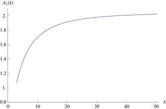
Figure 1. A plot of $A_{1}(k)$ for $3\leq k\leq 50$

Next, we use the estimate

$$(2k+3)(2k+4)(2k+5)>8(k+1)^{3},$$

which implies that

$$A_{1}(k)>\frac{2(k+1)}{k+6}\Bigl{(}\frac{8(k+1)^{2}}{\pi^{4}}\Bigr{)}^{1/(k+2)}$$

The first factor is greater than $1$ if $k\geq 5$ and the second one is greater than $1$ if $k\geq 3$. For $k=3$ get

$$A_{1}(3)=2^{14/5}3^{-8/5}5^{1/5}11^{1/5}\pi^{-4/5}\approx 1.07.$$

This finishes the proof of (3.8) and completes the proof. ∎

3.3. End of proof of Theorem 1.1

By Lemmas 2.2 and 2.4 it follows that

$$0<\alpha_{\text{min}}^{(k)}<\alpha_{\ast}^{(k)}.$$

However, by Lemmas 2.3 and 3.2, we find that all critical points in this interval must be non-degenerate minima. This clearly implies the uniqueness, and finishes the proof.∎

4. The case of even $k$

In this section we prove Theorem 1.2.

Proof (of Theorem 1.2).

The lower bound of $\lambda_{2,\mathfrak{Q}^{(k)}(\alpha)}$ from Lemma 5.1 is no good for small values of $\alpha$. Instead, we use the lower bound

$$\Bigl{(}\frac{t^{k+1}}{k+1}-\alpha\Bigr{)}^{2}\geq\Bigl{(}\frac{|t|^{k+1}}{k+1}-\alpha\Bigr{)}^{2},$$

and then we use that the second eigenvalue corresponding to the potential on the right-hand side on $\mathbb{R}$ is equal to the first eigenvalue of the operator

$$\mathfrak{Q}^{(k)}_{D}(\alpha)=-\frac{d^{2}}{dt^{2}}+\Bigl{(}\frac{t^{k+1}}{k+1}-\alpha\Bigr{)}^{2}$$

in $L^{2}(\mathbb{R}^{+})$ with a Dirichlet condition at $t=0$. We use the same type of splitting as in Lemma 3.2,

$$\mathfrak{Q}^{(k)}_{D}(\alpha)\geq\mathfrak{h}^{(k)}=\mathfrak{h}_{1}^{(k)}\oplus\mathfrak{h}_{2}^{(k)},$$

and write

$$0\leq\alpha<\varepsilon^{(k)}\widehat{\alpha}^{(k)}<\widehat{\alpha}^{(k)},\quad\hat{t}^{(k)}=(\widehat{\alpha}^{(k)}(k+1))^{1/(k+1)},$$

where the constants $\varepsilon^{(k)}$, $\widehat{\alpha}^{(k)}$ and $\hat{t}^{(k)}$ play the same roles as in the proof of Lemma 3.2 (but, as we will see, they are not the same!). This time the operator $\mathfrak{h}_{1}^{(k)}$ is given by

$$\mathfrak{h}_{1}^{(k)}=-\frac{d^{2}}{dt^{2}}$$

in $L^{2}((0,\hat{t}^{(k)}))$ with Dirichlet condition at $t=0$ and Neumann condition at $t=\hat{t}^{(k)}$. This operator has eigenvalues

$$\operatorname{Spec}\bigl{(}\mathfrak{h}_{1}^{(k)}\bigr{)}=\biggl{\{}\biggl{(}\frac{(2j-1)\pi}{2\hat{t}^{(k)}}\biggr{)}^{2}\biggr{\}}_{j\in\mathbb{N}\setminus\{0\}}.$$

The operator $\mathfrak{h}_{2}^{(k)}$ is the same as in the proof of Lemma 3.2, with eigenvalues

$$\operatorname{Spec}\bigl{(}\mathfrak{h}_{2}^{(k)}\bigr{)}=\biggl{\{}\biggl{[}\frac{2k(1-\varepsilon^{(k)})}{k+1}\bigl{(}\hat{t}^{(k)}\bigr{)}^{2k}\biggr{]}^{1/2}(4j-3)\biggr{\}}_{j\in\mathbb{N}\setminus\{0\}}$$

As in Lemma 3.2, the best lower bound we can get on $\lambda_{1,\mathfrak{Q}^{(k)}_{D}(\alpha)}$ is the one we get when the first eigenvalues of $\mathfrak{h}_{1}^{(k)}$ and $\mathfrak{h}_{2}^{(k)}$ are equal. This determines $\widehat{\alpha}^{(k)}$ as

$$\hat{t}^{(k)}=\biggl{[}\frac{\pi^{4}(k+1)}{32k(1-\varepsilon^{(k)})}\biggr{]}^{\frac{1}{2(k+2)}},\quad\widehat{\alpha}^{(k)}=\frac{1}{k+1}\biggl{[}\frac{\pi^{4}(k+1)}{32k(1-\varepsilon^{(k)})}\biggr{]}^{\frac{k+1}{2(k+2)}},$$ (4.1)

We let $\varepsilon^{(k)}=\frac{1}{2k}$. Then the lower bound becomes

$$\lambda_{2,\mathfrak{Q}^{(k)}_{N}(\alpha)}\geq\frac{\pi^{2}}{4}\biggl{[}\frac{32(k-1/2)}{\pi^{4}(k+1)}\biggr{]}^{\frac{1}{k+2}}.$$

To get the existence of an $\alpha_{\text{max}}^{(k)}>0$ such that condition (A) in Lemma 2.3 is fulfilled for $\alpha\in(-\alpha_{\text{max}}^{(k)},\alpha_{\text{max}}^{(k)})$ it is by Lemma 3.1 enough to show that $A_{2}(k)>1$ with

$$A_{2}(k):=\frac{k+2}{k+6}\frac{\frac{\pi^{2}}{4}\Bigl{[}\frac{32(k-1/2)}{\pi^{4}(k+1)}\Bigr{]}^{\frac{1}{k+2}}}{\bigl{(}\alpha_{\ast}^{(k)}\bigr{)}^{2}}=\frac{k+1}{k+6}\biggl{(}\frac{8}{\pi^{4}}(k-1/2)(2k+3)(2k+4)(2k+5)\biggr{)}^{1/(k+2)}.$$

See Figure 2 for a plot of $A_{2}(k)$ for $2\leq k\leq 50$. We note that $\lim_{k\to\infty}A_{2}(k)=1$.

Figure 2. A plot of $A_{2}(k)$ for $2\leq k\leq 50$

By using the estimate

$$(k-1/2)(2k+3)(2k+4)(2k+5)>16(k+1)^{3}$$

(which is valid for all $k\geq 2$) we find that $A_{2}(k)>B(k)$ with

$$B(k):=\frac{k+1}{k+6}\biggl{(}\frac{128}{\pi^{4}}(k+1)^{3}\biggr{)}^{1/(k+2)}.$$

The derivative of $B(k)$ is given by

$$B^{\prime}(k)=B(k)\frac{8k^{2}+44k+56-(k+1)(k+6)\log\bigl{(}\frac{128}{\pi^{4}}(k+1)^{3}\bigr{)}}{(k+1)(k+2)^{2}(k+6)}.$$

For $k\geq 14$ it holds that $\log\bigl{(}\frac{128}{\pi^{3}}(k+1)^{3}\bigr{)}>8$ and so

$$8k^{2}+44k+56-(k+1)(k+6)\log\Bigl{(}\frac{128}{\pi^{4}}(k+1)^{3}\Bigr{)}<8-12k\leq-160,$$

which implies that $B^{\prime}(k)<0$. Moreover, since $B(14)\approx 1.27$ and $\lim_{k\to\infty}B(k)=1$ it follows that $B(k)\geq 1$, and thus $A_{2}(k)>1$, for all $k\geq 14$.

For even $2\leq k\leq 12$, we calculate $A_{2}(k)$ numerically,

$k$	2	4	6	8	10	12
$A_{2}(k)$	1.05	1.41	1.49	1.50	1.49	1.47

which establishes $A_{2}(k)>1$ for all even $k\geq 2$.

The proof of the theorem is completed by an application of Lemma 2.3, noting that $\alpha=0$ is a critical point of $\lambda_{1,\mathfrak{Q}^{(k)}(\alpha)}$ since $\lambda_{1,\mathfrak{Q}^{(k)}(\alpha)}$ is even. ∎

5. The case of large $k$

The goal of this section is to prove Theorem 1.3. It will be done using the ideas from [5].

For even $k\geq 2$ we introduce

$$m_{k}=\inf_{t\in\mathbb{R}}\frac{t^{k+1}-1}{t-1}.$$ (5.1)

The constants $m_{k}$ decrease from $3/4$ for $k=2$ to $1/2$ as $k\to\infty$.

Lemma 5.1.

Let $k\geq 2$ be an even integer. With $m_{k}$ as in (5.1) it holds that

$$\lambda_{j,\mathfrak{Q}^{(k)}(\alpha)}\geq m_{k}\alpha^{k/(k+1)}(k+1)^{-1/(k+1)}(2j-1),\quad j\in\mathbb{N}\setminus\{0\}.$$ (5.2)

Proof.

We use a lower bound of the potential

$$\Bigl{(}\frac{t^{k+1}}{k+1}-\alpha\Bigr{)}^{2}=\alpha^{2}\biggl{(}\Bigl{(}\frac{t}{(\alpha(k+1))^{1/(k+1)}}\Bigr{)}^{k+1}-1\biggr{)}^{2}\\ \geq\Bigl{(}m_{k}\alpha^{k/(k+1)}(k+1)^{-1/(k+1)}\Bigr{)}^{2}\Bigl{(}t-(\alpha(k+1))^{1/(k+1)}\Bigr{)}^{2},$$

and then estimate with the eigenvalues of the harmonic oscillator on the whole line. ∎

Lemma 5.2.

Assume that $k\geq 2$ is an even integer and that $m_{k}$ is the constant from Lemma 5.1. Then $\alpha_{\text{min}}^{(k)}\leq\alpha_{\ast\ast}^{(k)}$ where

$$\alpha_{\ast\ast}^{(k)}\leq\biggl{[}\frac{(k+1)^{1/(k+1)}}{m_{k}}\biggl{(}\frac{\pi^{2}}{4}\frac{k+2}{k+1}\Bigl{(}\frac{1}{4}(k+1)(2k+3)(2k+4)(2k+5)\Bigr{)}^{-1/(k+2)}\biggr{)}\biggr{]}^{(k+1)/k}.$$ (5.3)

In particular, if $\eta>\frac{\pi^{2}}{2}$ then there exists $k_{0}$ such that, for $k\geq k_{0}$, $k$ even, $\lambda_{1,\mathfrak{Q}^{(k)}(\alpha)}$ attains its minimum in $(-\eta,\eta)$.

Proof.

Inequality (5.3) follows by combining Lemma 3.1 (with $\alpha=0$) with Lemma 5.1. The second statement is immediate, by letting $k\to\infty$, and using the fact that $m_{k}\geq\frac{1}{2}$ for all $k$. ∎

Lemma 5.3.

Let $\alpha>0$. For any $j\in\mathbb{N}\setminus\{0\}$ it holds that

$$\lim_{k\to\infty}\lambda_{j,\mathfrak{Q}^{(k)}(\alpha)}=\alpha^{2}+\Bigl{(}\frac{j\pi}{2}\Bigr{)}^{2}$$ (5.4)

with a uniform control with respect to $\alpha$ in any compact interval.

This result might be a consequence of $\Gamma$-convergence of the Pisa school, except possibly for the uniform control of $\alpha$. See also [12], in particular Example 4.2. For the sake of completeness, we give a proof inspired by the methods in [2].

Proof.

We start with the upper bound, which we prove for $j\leq 2$ only. The general proof uses the same argument.

For $j=1$ the upper bound follows from Lemma 3.1. For $j=2$, let us consider the functions

$$\varphi_{1}(t)=\begin{cases}\cos\bigl{(}\frac{\pi t}{2}\bigr{)}&\text{if $|t|\leq 1$}\\ 0&\text{if $|t|>1$},\end{cases}\quad\text{and}\quad\varphi_{2}(t)=\begin{cases}\sin(\pi t)&\text{if $|t|\leq 1$}\\ 0&\text{if $|t|>1$}.\end{cases}$$ (5.5)

They are eigenfunctions of the two lowest eigenvalues of the limiting model $k\to\infty$, $-\frac{d^{2}}{dt^{2}}+\alpha^{2}$ in $L^{2}((-1,1))$ with Dirichlet boundary conditions.

Computing the energy of the function $\mu_{1}\varphi_{1}+\mu_{2}\varphi_{2}$, $|\mu_{1}|^{2}+|\mu_{2}|^{2}=1$, we find a sphere in a two-dimensional space on which the energy is less than $\mu(k)$, with

$$\mu(k)=\alpha^{2}+\pi^{2}+C\frac{1+|\alpha|}{k+1}.$$

The upper bound in (5.4) for $j=2$ is a consequence of the min-max principle. We continue with the lower bound.

Let $\varepsilon>0$ be given. Then, for bounded $\alpha>0$, we can choose $k$ so large that

$$\Bigl{(}\frac{t^{k+1}}{k+1}-\alpha\Bigr{)}^{2}\geq p(t):=\begin{cases}\bigl{(}\frac{(1+\varepsilon)^{k+1}}{k+1}+\alpha\bigr{)}^{2},&\hphantom{-1-\varepsilon}\hbox to0.0pt{\hss$-\infty$}<t\leq-1-\varepsilon,\\ \alpha^{2}(1-\varepsilon),&-1-\varepsilon<t\leq 1-\varepsilon,\\ 0,&\hphantom{-}1-\varepsilon<t\leq 1+\varepsilon,\\ \bigl{(}\frac{(1+\varepsilon)^{k+1}}{k+1}-\alpha\bigr{)}^{2},&\hphantom{-}1+\varepsilon<t<\infty.\end{cases}$$

We want to solve the eigenvalue equation

$$-\frac{d^{2}}{dt^{2}}u+p(t)u=\lambda u,$$ (5.6)

by solving it for each interval and glue the solutions together as is done in several examples in [2]. We first note that the operator is positive, so we only have to consider $\lambda\geq 0$. Let us introduce the notation

$$A=\Bigl{(}\frac{(1+\varepsilon)^{k+1}}{k+1}+\alpha\Bigr{)}^{2},\quad B=\Bigl{(}\frac{(1+\varepsilon)^{k+1}}{k+1}-\alpha\Bigr{)}^{2},\quad C=\sqrt{\lambda-\alpha^{2}(1-\varepsilon)},$$

$$t_{0}=-1-\varepsilon,\quad t_{1}=1-\varepsilon,\quad t_{2}=1+\varepsilon.$$

We may choose $k$ so large that $A>\lambda$ and $B>\lambda$.

If $\lambda>\alpha^{2}(1-\varepsilon)$, the square integrable solution to (5.6) is given by

$$u(t)=\begin{cases}a_{0}\exp\bigl{(}\sqrt{A-\lambda}t\bigr{)}&-\infty<t\leq t_{0},\\ b_{0}\cos(Ct)+b_{1}\sin(Ct)&\hphantom{-\infty}\hbox to0.0pt{\hss$t_{0}$}<t\leq t_{1},\\ c_{0}\cos(\sqrt{\lambda}t)+c_{1}\sin(\sqrt{\lambda}t),&\hphantom{-\infty}\hbox to0.0pt{\hss$t_{1}$}<t\leq t_{2},\\ d_{0}\exp\bigl{(}-\sqrt{B-\lambda}t\bigr{)},&\hphantom{-\infty}\hbox to0.0pt{\hss$t_{2}$}<t<\infty.\end{cases}$$ (5.7)

Here $a_{0}$, $b_{0}$, $b_{1}$, $c_{0}$, $c_{1}$ and $d_{0}$ are constants that are determined by gluing the solution together. The conditions that both $u$ and $u^{\prime}$ should coincide at the points $t_{0}$, $t_{1}$ and $t_{2}$ read

$$a_{0}\exp\bigl{(}\sqrt{A-\lambda}t_{0}) =b_{0}\cos(Ct_{0})+b_{1}\sin(Ct_{0}),$$

$$a_{0}\sqrt{A-\lambda}\exp\bigl{(}\sqrt{A-\lambda}t_{0}) =-b_{0}C\sin(Ct_{0})+b_{1}C\cos(Ct_{0}),$$

$$b_{0}\cos(Ct_{1})+b_{1}\sin(Ct_{1}) =c_{0}\cos(\sqrt{\lambda}t_{1})+c_{1}\sin(\sqrt{\lambda}t_{1}),$$

$$-b_{0}C\sin(Ct_{1})+b_{1}C\cos(Ct_{1}) =-c_{0}\sqrt{\lambda}\sin(\sqrt{\lambda}t_{1})+c_{1}\sqrt{\lambda}\cos(\sqrt{\lambda}t_{1}),$$

$$c_{0}\cos(\sqrt{\lambda}t_{2})+c_{1}\sin(\sqrt{\lambda}t_{2}) =d_{0}\exp\bigl{(}-\sqrt{B-\lambda}t_{2}\bigr{)},$$

$$-c_{0}\sqrt{\lambda}\sin(\sqrt{\lambda}t_{2})+c_{1}\sqrt{\lambda}\cos(\sqrt{\lambda}t_{2}) =-d_{0}\sqrt{B-\lambda}\exp\bigl{(}-\sqrt{B-\lambda}t_{2}\bigr{)}.$$

This is a linear system of equations in $a_{0}$, $b_{0}$, $b_{1}$, $c_{0}$, $c_{1}$ and $d_{0}$ which has nontrivial solutions if and only if

$$\frac{1}{C}\frac{\sqrt{A-\lambda}\tan\bigl{(}C(t_{1}-t_{0})\bigr{)}+C}{\sqrt{A-\lambda}-C\tan\bigl{(}C(t_{1}-t_{0})\bigr{)}}=-\frac{1}{\lambda}\frac{\sqrt{B-\lambda}\tan\bigl{(}\sqrt{\lambda}(t_{2}-t_{1})\bigr{)}+\sqrt{\lambda}}{\sqrt{B-\lambda}-\sqrt{\lambda}\tan\bigl{(}\sqrt{\lambda}(t_{2}-t_{1})\bigr{)}}$$ (5.8)

This is the equation that determines the eigenvalues $\lambda$. For large $k$, the terms $\sqrt{A-\lambda}$ and $\sqrt{B-\lambda}$ are dominating, and we can write (5.8) as

$$\frac{1}{C}\tan\bigl{(}C(t_{1}-t_{0})\bigr{)}=-\frac{1}{\sqrt{\lambda}}\tan\bigl{(}\sqrt{\lambda}(t_{2}-t_{1})\bigr{)}+\mathcal{O}\bigl{(}(k+1)(1+\varepsilon)^{-(k+1)}\bigr{)}$$ (5.9)

as $k\to\infty$, where the estimate is uniform for bounded $\alpha$ and $\lambda$. Inserting the values for $t_{0}$, $t_{1}$, $t_{2}$ and $C$, we find that

$$\frac{1}{\sqrt{\lambda-\alpha^{2}(1-\varepsilon)}}\tan\bigl{(}2\sqrt{\lambda-\alpha^{2}(1-\varepsilon)}\bigr{)}=-\frac{1}{\sqrt{\lambda}}\tan\bigl{(}2\varepsilon\sqrt{\lambda}\bigr{)}+\mathcal{O}\bigl{(}(k+1)(1+\varepsilon)^{-(k+1)}\bigr{)}.$$ (5.10)

If $0<\lambda<\alpha^{2}(1-\varepsilon)$ then hyperbolic functions appear in the solution of (5.6), and the same type of calculations that resulted in (5.10) this time yield

$$\frac{1}{\sqrt{\alpha^{2}(1-\varepsilon)-\lambda}}\tanh\bigl{(}2\sqrt{\alpha^{2}(1-\varepsilon)-\lambda}\bigr{)}=-\frac{1}{\sqrt{\lambda}}\tan\bigl{(}2\varepsilon\sqrt{\lambda}\bigr{)}+\mathcal{O}\bigl{(}(k+1)(1+\varepsilon)^{-(k+1)}\bigr{)}.$$

The function

$$f_{1}(\lambda)=\begin{cases}\frac{1}{\sqrt{\alpha^{2}(1-\varepsilon)-\lambda}}\tanh\bigl{(}2\sqrt{\alpha^{2}(1-\varepsilon)-\lambda}\bigr{)},&0<\lambda<\alpha^{2}(1-\varepsilon),\\ 2,&\lambda=\alpha^{2}(1-\varepsilon),\\ \frac{1}{\sqrt{\lambda-\alpha^{2}(1-\varepsilon)}}\tan\bigl{(}2\sqrt{\lambda-\alpha^{2}(1-\varepsilon)}\bigr{)},&\alpha^{2}(1-\varepsilon)<\lambda<\infty,\end{cases}$$

is positive for all $0\leq\lambda<\alpha^{2}(1-\varepsilon)+\frac{\pi^{2}}{16}$, and $\lim_{\lambda\nearrow\alpha^{2}(1-\varepsilon)+\frac{\pi^{2}}{16}}f_{1}(\lambda)=+\infty$. For larger $\lambda$ it holds that $f_{1}(\lambda)$ is monotonically increasing from $-\infty$ to $+\infty$ in every interval

$$\biggl{(}\biggl{[}\frac{(j-1/2)\pi}{2}\biggr{]}^{2}+\alpha^{2}(1-\varepsilon),\biggl{[}\frac{(j+1/2)\pi}{2}\biggr{]}^{2}+\alpha^{2}(1-\varepsilon)\biggr{)}.$$ (5.11)

The function

$$f_{2}(\lambda)=-\frac{1}{\sqrt{\lambda}}\tan\bigl{(}2\varepsilon\sqrt{\lambda}\bigr{)}$$

is negative for all $0\leq\lambda<\bigl{(}\frac{\pi}{4\varepsilon}\bigr{)}^{2}$, and $\lim_{\lambda\nearrow\bigl{(}\frac{\pi}{4\varepsilon}\bigr{)}^{2}}f_{2}(\lambda)=-\infty$.

We find that if $\varepsilon$ satisfies

$$\Bigl{(}\frac{\pi}{4\varepsilon}\Bigr{)}^{2}>\biggl{[}\frac{(j+1/2)\pi}{2}\biggr{]}^{2}+\alpha^{2}(1-\varepsilon)$$

then there exists a $k_{j}(\varepsilon)$ and $C_{j}$ such that if $k\geq k(\varepsilon)$, $k$ even, it holds that the $j$th solution of (5.10) lies in the interval (5.11) and we conclude that

$$\lambda_{j,\mathfrak{Q}^{(k)}(\alpha)}\geq\biggl{[}\frac{(j-1/2)\pi}{2}\biggr{]}^{2}+\alpha^{2}(1-\varepsilon)-C_{j}\varepsilon.$$

This is not the upper bound we wanted. However we can do better. There exists a constant $K_{j}>0$ (uniform in $\alpha$, $\varepsilon$) such that

$$0<\lambda<\biggl{[}\frac{(j+1/2)\pi}{2}\biggr{]}^{2}+\alpha^{2}(1-\varepsilon)\implies-K_{j}\varepsilon<f_{2}(\lambda)<0.$$

This implies that the first $j$ solutions to (5.10), up to an error of order $\varepsilon$ coincide with the first $j$ zeros of the function $f_{1}(\lambda)$, i.e., for all $\varepsilon>0$ there exist $\hat{k}_{j}(\varepsilon)$ and $\widehat{C}_{j}$ such that for $k\geq\hat{k}_{j}(\varepsilon)$, $k$ even, it holds that

$$\lambda_{j,\mathfrak{Q}^{(k)}(\alpha)}\geq\Bigl{(}\frac{j\pi}{2}\Bigr{)}^{2}+\alpha^{2}(1-\varepsilon)-\widehat{C}_{j}\varepsilon.$$

This completes the proof of (5.4). ∎

We are now ready to prove Theorem 1.3.

Proof (of Theorem 1.3).

First, we show (1.3), where we consider odd $k$ only. We recall the bound (3.11) on $\alpha_{\text{min}}^{(k)}$, $0<\alpha_{\text{min}}^{(k)}<\sqrt{\frac{5}{4}}\frac{\pi}{2}$, and the formula (2.3) which is valid for $\alpha_{\text{min}}^{(k)}$, i.e.,

$$\alpha_{\text{min}}^{(k)}=\int_{\mathbb{R}}\frac{t^{k+1}}{k+1}\bigl{(}u_{1,\alpha_{\text{min}}^{(k)}}\bigr{)}^{2}\,\mathrm{d}t.$$

It is enough to show that

$$\lim_{k\to\infty}\int_{1}^{\infty}\frac{t^{k+1}}{k+1}\bigl{(}u_{1,\alpha_{\text{min}}^{(k)}}\bigr{)}^{2}\,\mathrm{d}t=0.$$

We first show that, for any $\varepsilon>0$ it holds that

$$\lim_{k\to\infty}\int_{1+\varepsilon}^{\infty}\frac{t^{k+1}}{k+1}\bigl{(}u_{1,\alpha_{\text{min}}^{(k)}}\bigr{)}^{2}\,\mathrm{d}t=0.$$ (5.12)

For any $k\geq 3$ and $0<\alpha<\sqrt{\frac{5}{4}}\frac{\pi}{2}$ we use Lemma 3.1 to find

$$\int_{1+\varepsilon}^{\infty}\frac{t^{2(k+1)}}{(k+1)^{2}}\bigl{(}u_{1,\alpha}\bigr{)}^{2}\,\mathrm{d}t\leq 2\int_{1+\varepsilon}^{\infty}\Bigl{(}\frac{t^{k+1}}{k+1}-\alpha\Bigr{)}^{2}\bigl{(}u_{1,\alpha}\bigr{)}^{2}\,\mathrm{d}t\\ +2\alpha^{2}\leq 2\lambda_{1,\mathfrak{Q}^{(k)}(\alpha)}+2\alpha^{2}<\frac{15}{8}\pi^{2}.$$ (5.13)

In particular, we get

$$\int_{1+\varepsilon}^{\infty}\frac{t^{k+1}}{k+1}\bigl{(}u_{1,\alpha_{\text{min}}^{(k)}}\bigr{)}^{2}\,\mathrm{d}t\leq(1+\varepsilon)^{-(k+1)}(k+1)\frac{15}{8}\pi^{2},$$

which establishes (5.12). We write the remaining integral as

$$\int_{1}^{1+\varepsilon}\frac{t^{k+1}}{k+1}\bigl{(}u_{1,\alpha_{\text{min}}^{(k)}}\bigr{)}^{2}\,\mathrm{d}t=\\ \int_{1}^{1+\varepsilon}\Bigl{(}\frac{t^{k+1}}{k+1}-\alpha_{\text{min}}^{(k)}\Bigr{)}\bigl{(}u_{1,\alpha_{\text{min}}^{(k)}}\bigr{)}^{2}\,\mathrm{d}t+\alpha_{\text{min}}^{(k)}\int_{1}^{1+\varepsilon}\bigl{(}u_{1,\alpha_{\text{min}}^{(k)}}\bigr{)}^{2}\,\mathrm{d}t,$$

and apply the Cauchy-Schwarz inequality and use (2.6) to conclude that the first integral tends to zero as $k\to\infty$. For the second integral we use the general inequality

$$\int_{a}^{b}u(t)^{2}\,\mathrm{d}t\leq 4\int_{\frac{a+b}{2}}^{b}u(t)^{2}\,\mathrm{d}t+2(b-a)^{2}\int_{a}^{b}u^{\prime}(t)^{2}\,\mathrm{d}t$$

with $a=1$ and $b=1+\varepsilon$. We use (5.13) to find that

$$\int_{1+\frac{\varepsilon}{2}}^{1+\varepsilon}\bigl{(}u_{1,\alpha_{\text{min}}^{(k)}}\bigr{)}^{2}\,\mathrm{d}t\leq\Bigl{(}1+\frac{\varepsilon}{2}\Bigr{)}^{-2(k+1)}(k+1)^{2}\int_{1+\frac{\varepsilon}{2}}^{\infty}\frac{t^{2(k+1)}}{(k+1)^{2}}\bigl{(}u_{1,\alpha_{\text{min}}^{(k)}}\bigr{)}^{2}\,\mathrm{d}t\\ \leq\frac{15}{8}\pi^{2}\Bigl{(}1+\frac{\varepsilon}{2}\Bigr{)}^{-2(k+1)}(k+1)^{2}.$$

Moreover we use the inequality

$$\int_{1}^{1+\varepsilon}\bigl{(}u_{1,\alpha_{\text{min}}^{(k)}}^{\prime}\bigr{)}^{2}\,\mathrm{d}t\leq\lambda_{1,\mathfrak{Q}^{(k)}(\alpha_{\text{min}}^{(k)})}\leq\frac{5}{16}\pi^{2},$$

to get, finally,

$$\int_{1}^{1+\varepsilon}\bigl{(}u_{1,\alpha_{\text{min}}^{(k)}}\bigr{)}^{2}\,\mathrm{d}t\leq\frac{15}{2}\pi^{2}\Bigl{(}1+\frac{\varepsilon}{2}\Bigr{)}^{-2(k+1)}(k+1)^{2}+\frac{5}{8}\pi^{2}\varepsilon^{2}.$$

This achieves the proof of (1.3).

We continue with the proof of the second statement. We know that $\alpha=0$ is a non-degenerate local minima. By Lemma 5.2 it is enough to show that there exists a $k_{0}$ such that condition (A) in Lemma 2.3 holds for all $k\geq k_{0}$, $k$ even, and all $0<\alpha\leq\eta$, where $\eta>\frac{\pi^{2}}{2}$ is arbitary. However, it is clear by Lemma 5.3 that this can be done. ∎

References

- [1] J. Aramaki. Asymptotics of eigenvalue for the Ginzburg-Landau operator in an applied magnetic field vanishing of higher order. Int. J. Pure Appl. Math. Sci., 2(2):257–281, 2005.
- [2] S. Flügge. Practical Quantum Mechanics. Classics in Mathematics. Springer-Verlag, Berlin, English edition, 1999. Translated from the 1947 German original.
- [3] B. Helffer. The Montgomery model revisited. To appear in Colloquium Mathematicum, volume in honor of A. Hulanicki, 2009.
- [4] B. Helffer and Y. A. Kordyukov. Spectral gaps for periodic Schrödinger operators with hypersurface magnetic wells. In Mathematical results in quantum mechanics, pages 137–154. World Sci. Publ., Hackensack, NJ, 2008.
- [5] B. Helffer and Y. A. Kordyukov. Complements on Montgomery like model : . Unpublished notes, 2009.
- [6] B. Helffer and Y. A. Kordyukov. Semi-classical analysis of Schrödinger operators with magnetic wells. To appear in Contemporary Mathematics, 2009.
- [7] B. Helffer and Y. A. Kordyukov. Spectral gaps for periodic Schrödinger operators with hypersurface magnetic wells: Analysis near the bottom. J. Funct. Anal., 257:3043–3081, 2009.
- [8] B. Helffer and A. Morame. Magnetic bottles in connection with superconductivity. J. Funct. Anal., 185(2):604–680, 2001.
- [9] B. Helffer and J. Sjöstrand. Multiple wells in the semiclassical limit. I. Comm. Partial Differential Equations, 9(4):337–408, 1984.
- [10] R. Montgomery. Hearing the zero locus of a magnetic field. Comm. Math. Phys., 168(3):651–675, 1995.
- [11] X.-B. Pan and K.-H. Kwek. Schrödinger operators with non-degenerately vanishing magnetic fields in bounded domains. Trans. Amer. Math. Soc., 354(10):4201–4227 (electronic), 2002.
- [12] B. Simon. A canonical decomposition for quadratic forms with applications to monotone convergence theorems. J. Funct. Anal., 28(3):377–385, 1978.
- [13] B. Simon. Semiclassical analysis of low lying eigenvalues. I. Nondegenerate minima: asymptotic expansions. Ann. Inst. H. Poincaré Sect. A (N.S.), 38(3):295–308, 1983.