Exchange flow of two immiscible fluids and the principle of maximum flux

Abstract

The steady, coaxial flow in which two immiscible, incompressible fluids move past each other in a cylindrical tube has a continuum of possibilities due to the arbitrariness of the interface between the fluids. By invoking the presence of surface tension to at least restrict the shape of any interface to that of a circular arc or full circle, we consider the following question: which flow will maximise the exchange when there is only one dividing interface $\Gamma$? Surprisingly, the answer differs fundamentally from the better-known co-directional two-phase flow situation where an axisymmetric (concentric) core-annular solution always optimises the flux. Instead, the maximal flux state is invariably asymmetric either being a ‘side-by-side’ configuration where $\Gamma$ starts and finishes at the tube wall or an eccentric core-annular flow where $\Gamma$ is an off-centre full circle in which the more viscous fluid is surrounded by the less viscous fluid. The side-by-side solution is the most efficient exchanger for a small viscosity ratio $\beta\lesssim 4.60$ with an eccentric core-annular solution optimal otherwise. At large $\beta$, this eccentric solution provides 51% more flux than the axisymmetric core-annular flow which is always a local minimiser of the flux.

1 Introduction

For Newtonian fluids at least where the governing Navier-Stokes equations are known, the most fundamental issue in fluid mechanics is predicting the realised flow solution for a given initial state and set of boundary conditions against a background of omnipresent noise. Non-uniqueness of solution is endemic due to the nonlinearity of the Navier-Stokes equations but even in special limits (e.g. vanishing Reynolds number or steady, unidirectional flow) where these simplify to the linear Stokes’ equations, degeneracy is rife as specification of the flow domain is typically part of the problem. A well-known example of this is the pressure-driven flow of two immiscible fluids along a cylindrical tube (e.g. Joseph, Renardy & Renardy 1984, Joseph, Nguyen and Beavers 1984, and Joseph et al. 1997). Here there is a continuum of steady unidirectional solutions possible due to the arbitrariness in the interface between the two fluids. In practice, however, the axisymmetric core-annular solution with the more viscous fluid surrounded by the less viscous fluid is invariably observed for fluid combinations ranging from oil and water (Charles & Redberger 1962, Yu & Sparrow 1967, Hasson, Mann & Nir 1970), to molten polymers (Southern & Ballman 1973, Everage 1973, Lee & White 1974, Williams 1975 and Minagawa & White 1975).

Interestingly, it appears that if an extra constraint is added to the system - that the mean volumetric flux along the tube vanishes - different steady solutions are observed (Arakeri et al. 2000, Huppert & Hallworth 2007, Beckett et al. 2009). Such a flow is easily set up in the laboratory by placing a tank of dense fluid directly above a tank full of less dense fluid and connecting the two by a vertical cylindrical tube. If the density difference or the tube cross-section is small enough or the fluid viscosities large enough, it is reasonable to anticipate a steady, coaxial flow established in the tube in which the denser fluid falls under gravity displacing the less dense fluid upwards. When the lower tank is initially full and both fluids incompressible, this exchange flow is constrained to have no net volume flux along the tube. As in the unidirectional flow situation, the form of the steady, coaxial two-fluid flow realised is fascinatingly unclear due to the arbitrariness of the interface between the fluids (formally, any union of open curves terminating on the tube wall and closed curves in the interior are possible). Using salty and pure water, Arakeri et al (2000) saw only a ‘half-and-half’ solution where the interface divides the tube cross-section into two approximately equal domains (hereafter referred to as a ‘side-by-side’ solution). In contrast, Huppert & Hallworth (2007) saw only a concentric core-annular flow as their steady low-Reynolds solution and recently both types of flow have been seen in the same apparatus (Beckett et al. 2009). Beyond its intrinsic interest, this flow has applications ranging from the exchange of degassed and gas-rich magma in volcanoes (e.g. see Huppert & Hallworth 2007 and references herein) to plug-cementing oilfields (e.g. Frigaard & Scherzer 1998, Moyers-Gonzalez & Frigaard 2004). There is also associated work on exchange problems involving miscible fluids, tilted tubes or channels, and unsteady solutions (see the recent articles by Seon et al. 2007, Znaien et al. 2009 and Taghavi et al. 2009 for references).

Resolving the flow degeneracy of the steady state in favour of one realised solution involves knowledge of the initial conditions of the exchange flow, the pressure boundary conditions set-up across the tube and the inherent instability mechanisms present. Pragmatically, the initial conditions are never known that well (e.g. barriers are slid open or plugs removed in the laboratory), the pressure gradient which gets set up difficult to measure and assessing relative stability requires every possible flow state to be identified first. It is therefore tempting to jump to an ad-hoc selection principle especially as a particularly obvious one suggests itself here: the flow selects the solution which has the largest individual volumetric flux. A selection principle based upon maximum flux has some history in the undirectional two-phase flow problem motivated by its formal connection to the single fluid problem (Maclean 1973, Everage 1973, Joseph, Nguyen & Beavers 1984). Here, the governing Stokes equations are the Euler-Lagrange equations for maximising the flux for velocity fields which satisfy the global power balance that the rate at which energy is viscously dissipated equals the power supplied by the applied pressure gradient (per unit length of the tube). Specifically, if $G$ is the constant applied pressure gradient, $\Omega$ the cross-section of the tube and $u$ the speed along the tube, then

$$\mu\nabla^{2}u=G\qquad\Leftrightarrow\qquad\delta\int_{\Omega}\,u+\Lambda(\mu|\nabla u|^{2}+Gu)\,dA=0$$ (1)

where $\delta$ indicates the Frechét (variational) derivative, $\int\,-Gu\,dA$ is the rate of working by the pressure gradient per unit length of tube and the Lagrange multiplier $\Lambda$ imposing the power balance constraint takes the value $1/G$. The stationary point defined by the variational solution is clearly one of maximum flux because the only quadratic term in the integrand is negative definite ($u$ is oppositely signed to $G$ so $\Lambda<0$). The fact that this variational formulation can be extended to two fluids provided the interface between them is known (Maclean 1973, Everage 1973) supplied the impetus to invoke the principle of maximal flux more generally. It appears to be mostly successful - in the words of Joseph, Nguyen and Beavers (1984) “our experiments show that something like this is going on”- predicting that the more viscous fluid will be encircled by the less viscous fluid which then acts as a lubricant against the tube walls (see also Charles & Redberger 1962, Yu & Sparrow 1967, Hasson, Mann & Nir 1970, Southern & Ballman 1973, Everage 1973, Lee & White 1974, Williams 1975, Minagawa & White 1975). Joseph, Renardy & Renardy (1984), however, add some qualifications: this state can become unstable if the more viscous core gets too small.

Given this history, the purpose of this paper is to explore the consequences of this ‘maximum flux principle’ in predicting the form of the exchange flow realised in a vertical cylindrical tube. Formally solving the variational problem with the interface (or interfaces) as an unknown is a formidable challenge not attempted here. Rather, a survey is conducted over a physically-motivated subspace of all mathematically-possible steady, coaxial solutions. This subspace is defined by two (mild) assumptions: a) the fluids occupy one (possibly multi-connected) domain so that there is only one interface $\Gamma$, and b) that this interface is a circular arc or a full circle. The motivation for the former assumption is stability - multiple small fluid domains would presumably aggregate - and the presence of some surface tension between the two fluids conveniently motivates the latter. The axially-constant, lateral pressure difference required to balance interfacial tension, however, will be ignored in what follows as it has no consequence for the calculations.

2 Formulation

Consider two immiscible fluids with densities $\rho_{1}$ and $\rho_{2}$ and viscosities $\mu_{1}$ and $\mu_{2}$ which are flowing in a vertical circular tube of radius $a$ across which there is a pressure gradient $G$ and $g$ is the acceleration due to gravity. Assuming that fluid 1(2) occupies an area $A^{*}_{1}$($A^{*}_{2}$), the Navier-Stokes equations for steady exchange flow of the two fluids either directed up or down the tube (so the problem is just in the cross-sectional plane) are

$$G=\mu_{1}\nabla^{2}u^{*}_{1}-\rho_{1}g\quad{\rm in}\quad A^{*}_{1},\qquad G=\mu_{2}\nabla^{2}u^{*}_{2}-\rho_{2}g\quad{\rm in}\quad A^{*}_{2}$$ (2)

with non-slip boundary conditions at the tube wall and continuity of velocity and stress at the interface $\Gamma^{*}$ between the two fluids, that is

$$u^{*}_{1}=u^{*}_{2}\quad\&\quad\mu_{1}\frac{\partial u^{*}_{1}}{\partial n}=\mu_{2}\frac{\partial u^{*}_{2}}{\partial n}\quad{\rm on\quad\Gamma^{*}}$$ (3)

(where $\partial/\partial n$ is the normal derivative to $\Gamma^{*}$). There is a further constraint that the net volume flux through the tube is zero so

$$Q^{*}:=-\int\,u^{*}_{1}\,dA^{*}_{1}=\int\,u^{*}_{2}\,dA^{*}_{2}.$$ (4)

Without loss of generality, we assume $\rho_{1}>\rho_{2}$ so that $Q^{*}$ is positive (the less dense fluid rises). This does not prejudice the choice of viscosities later because of the symmetry $(\rho_{1},\rho_{2},g)\rightarrow(\rho_{2},\rho_{1},-g)$: the direction ‘up’ is irrelevant with only the density difference being important.

The system is non-dimensionalised (*’s removed) using the tube radius $a$, the differential hydrostatic pressure gradient $\Delta\rho g$ (where $\Delta\rho:=\rho_{1}-\rho_{2}$) and $\mu_{1}$ so that after defining $\lambda$ by

$$G=-\mbox{$\frac{1}{2}$}(\rho_{1}+\rho_{2})g+\mbox{$\frac{1}{2}$}\Delta\rho g\lambda$$ (5)

then

$$\nabla^{2}u_{1} = \lambda+1\quad{\rm in}\quad A_{1},$$ (6)

$$\beta\nabla^{2}u_{2} = \lambda-1\quad{\rm in}\quad A_{2},$$ (7)

$$u_{1}=u_{2}\quad\&\quad\frac{\partial u_{1}}{\partial n}=\beta\frac{\partial u_{2}}{\partial n}\quad{\rm on\quad\Gamma}.$$ (8)

where

$$\beta:=\frac{\mu_{2}}{\mu_{1}}.$$ (9)

Henceforth $u_{1}$ and $u_{2}$ are in units of $\mbox{$\frac{1}{2}$}\Delta\rho ga^{2}/\mu_{1}$ and the one-fluid volume flux

$$Q:=-\int\,u_{1}\,dA_{1}=\int\,u_{2}\,dA_{2}$$ (10)

is in units of $\mbox{$\frac{1}{2}$}\Delta\rho ga^{4}/\mu_{1}$ with $A_{1}\cup A_{2}$ being the unit disk.

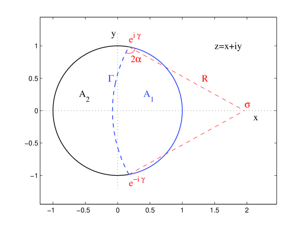
Figure 1: The side-by-side solution configuration specified by two parameters: $\gamma$ and $\alpha$.

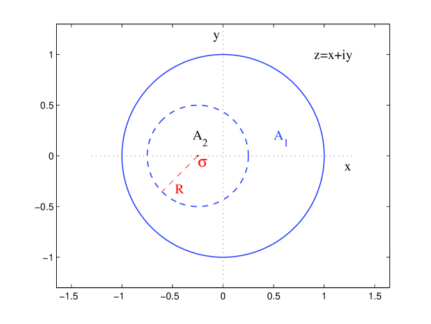
Figure 2: The eccentric core-annular configuration specified by two parameters: $\sigma$ and $R$.

Two specific choices are now made for $\Gamma$. The first is a circular arc of general curvature and position which intersects the tube wall so that the two fluids are next to each other - the side-by-side solution: see figure 1. The second is a full circle completely contained within, but not concentric with, the tube so that one fluid encapsulates the other - the eccentric core-annular solution: see figure 2. The limiting case of a concentric core-annular solution needs to be treated separately but is easily solved analytically.

2.1 Side-by-side solutions

The geometry of the side-by-side solution is shown in figure 1 to be defined by two parameters: $\gamma$, the (upper) intercept latitude of $\Gamma$ with the tube wall, and $2\alpha$, the angle between $\Gamma$ and tube wall. For given viscosity ratio $\beta$ and pressure gradient $\lambda$, one of these (nominally $\alpha$) is determined by the flux balance leaving a 1-dimensional family of side-by-side flows with corresponding fluxes $Q=Q_{s}(\beta,\lambda;\gamma)$ possible (see appendix A for the calculation details). There is a symmetry

$$Q(\beta,\lambda;\gamma,\alpha)=\frac{1}{\beta}Q(\frac{1}{\beta},-\lambda;\pi-\gamma,\frac{\pi}{2}-\alpha)$$ (11)

which means that only $\beta\geq 1$ need be considered providing the full ranges of $\gamma$ and $\alpha$ are studied. Henceforth fluid 2 will always be the more viscous fluid so that the non-dimensionalisation has been done using the smaller dynamic viscosity $\mu_{1}$.

2.2 Eccentric solutions

The eccentric core-annular solution has one fluid domain as a totally-contained circular disk (cylinder) not touching the tube wall. The radius $R<1$ and centre $(\sigma,0)$ of $\Gamma$ define the geometry uniquely up to obvious rotations and reflections. To match smoothly onto the choices made in the side-by-side solution, $\sigma$ is chosen to be +ve(-ve) for $A_{1}$ in $A_{2}$ ($A_{2}$ in $A_{1}$). As before, for given viscosity ratio $\beta$ and pressure gradient $\lambda$, one of these two geometrical parameters is determined by the flux balance. This is done by searching over $R$ for given

$$d:=\biggl{\{}\begin{array}[]{rl}1+\sigma-R&\qquad A_{2}\quad{\rm in}\quad A_{1}\qquad\sigma<0\\ -1+\sigma+R&\qquad A_{1}\quad{\rm in}\quad A_{2}\qquad\sigma>0\end{array}\biggr{.}$$ (12)

which either represents the positive displacement from $(-1,0)$ to $(\sigma-R,0)$, the leftmost point of $\Gamma$ for the case of $A_{2}$ in $A_{1}$ ($\sigma<0$) , or the negative displacement of $(\sigma+R,0)$, the rightmost point of $\Gamma$, from $(1,0)$ for the case of $A_{1}$ in $A_{2}$ ($\sigma>0$). This choice is made for two reasons. Firstly, $d$ is a convenient way of extending the side-by-side solutions continuously beyond their pinch-off points into the corresponding eccentric solutions: $\gamma\rightarrow 0$ corresponds to $A_{2}$ encapsulating $A_{1}$ and $d$ decreasing across zero whereas $\gamma\rightarrow\pi$ corresponds to $A_{1}$ encapsulating $A_{2}$ and $d$ increasing across zero (see figure 3). Secondly, only one flux-balanced solution was ever found for a given $d$ whereas some $\sigma$ can have two flux-balanced solutions. The result is that two 1-dimensional families of eccentric core-annular flows with corresponding fluxes $Q_{e}(\beta,\lambda;d)$ (more viscous core) and $\hat{Q}_{e}(\beta,\lambda,d)$ (less viscous core) are possible (see appendix B for the calculation details). It’s worth re-emphasizing here that $\beta\geq 1$ so all the flux values quoted are in units of $1/\mu_{1}$ where $\mu_{1}$ is the smaller dynamic viscosity.

2.3 Concentric solutions

When $\Gamma$ is a circle concentric with the tube wall there is a simple solution to the problem (6)-(8) discussed recently by Huppert & Hallworth (2007):

$$u_{1} = \frac{\lambda+1}{4}(r^{2}-1)-R^{2}\log r,\hskip 85.35826ptR\leq r\leq 1$$ (13)

$$u_{2} = \frac{\lambda-1}{4\beta}(r^{2}-R^{2})-R^{2}\log R-\frac{\lambda+1}{4}(1-R^{2}).\qquad r\leq R$$ (14)

The associated fluxes are

$$Q_{1} = \frac{\pi}{8}\biggl{[}(\lambda+1)(2R^{2}-R^{4}-1)+4R^{2}(1-R^{2})+8R^{4}\log R\biggr{]},$$ (15)

$$Q_{2} = \frac{\pi}{8\beta}\biggl{[}(1-\lambda)R^{4}-2\beta(1+\lambda)R^{2}(1-R^{2})-8\beta R^{4}\log R\biggr{]}.$$ (16)

Since this is a special case of an eccentric core-annular solution with $\sigma=0$, there is unique $0<R<1$ for a flux-balanced solution which is

$$R_{c}=\sqrt{\frac{2\beta-\sqrt{4\beta^{2}-\beta(1+\lambda)[\beta(3-\lambda)+(\lambda-1)]}}{[\beta(3-\lambda)+(\lambda-1)]}}.$$ (17)

so that the flux (for fluid 2 in the core) is $Q_{c}(\beta,\lambda)$. As $\beta\rightarrow\infty$,

$$R_{c}\rightarrow\sqrt{(1+\lambda)/(3-\lambda)},\qquad\lambda\rightarrow 0.1746\qquad{\rm and}\quad Q_{c}\rightarrow 0.01831$$ (18)

from above. The opposite scenario of the less viscous fluid (fluid 1) in the core has $Q:=\hat{Q}_{c}\sim O(\beta)$ ($\beta\rightarrow 1/\beta$ in expressions (15) and (16) and multiply $Q$ by $1/\beta$ to convert the flux units to those using the smaller dynamic viscosity).

2.4 Strategy

The strategy now is to calculate $max_{\lambda}Q$ as a function of $\beta$ over all possible geometries smoothly ranging from the concentric solution with less viscous fluid in the core through to the concentric solution with the more viscous fluid in the core. Figure 3 illustrates the spectrum of possibilities and a glimpse of how the flux varies at one $\beta$ value. Before detailing the results further, the reader may be amused by an admission. At onset, this author (naively?) expected the calculation of maximum flux to be a simple competition between a local maximum achieved by the side-by-side solution and the flux $Q_{c}$ associated with the concentric core-annular flow influenced by the known behaviour of unidirectional 2-fluid flow. The side-by-side solution, however, quickly loses its interior maximum ($0<\gamma<\pi$) as $\beta$ increases in favour of an end-point maximum at $\gamma=\pi$. The fact that this end-point maximum exceeds the concentric solution flux $Q_{c}$ unequivocally indicated the importance of the intermediate eccentric core-annular flux $Q_{e}$.

Figure 3: The flux ${\rm max}_{\lambda}Q$ plotted across the various flow configurations ($d<0$ indicates less viscous core and $d>0$ more viscous core) for $\beta=5$. The leftmost point is $\hat{Q}_{c}$, beyond this, the region $d<0$ is the domain for $\hat{Q}_{e}$, the region $\gamma\in[0,\pi]$ is the domain for $Q_{s}$, $d>0$ the domain for $Q_{e}$ and the rightmost point is $Q_{c}$. The interior local maxima are highlighted with dots. The curve is only $C^{0}$ because the abscissa changes character at $\gamma=0$ and $\pi$ of course.

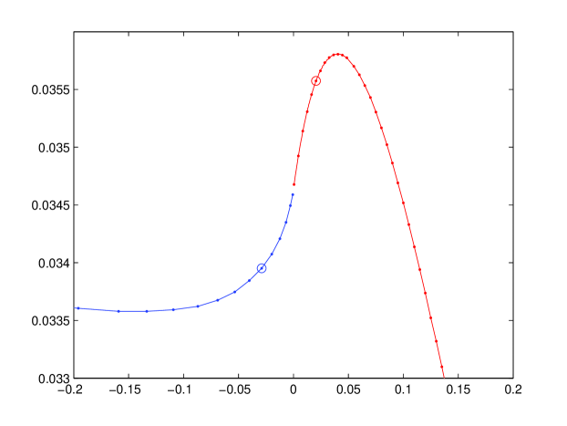
Figure 4: Plotting ${\rm max}_{\lambda}Q$ against $d$ at $\beta=5$ for side-by-side solutions as $d\rightarrow 0^{-}$ ($\gamma\rightarrow\pi$) and eccentric solutions as $d\rightarrow 0^{+}$ demonstrates the smooth connection between the two formulations. Velocity fields for the circled points are shown in figure 5.

Figure 5: The pinching-off side-by-side ($d=-0.0198$, $-0.051\leq u\leq 0.041$) and near-touching eccentric solutions ($d=0.0205$, $-0.052\leq u\leq 0.043$) for $\beta=5$ and the optimal $\lambda=-0.20$ corresponding to the circles in figure 4. The contours range from -0.105 (dark/red) to 0.105 (light/white) in steps of 0.01 here and throughout figures 7 and 8 to aid comparison.

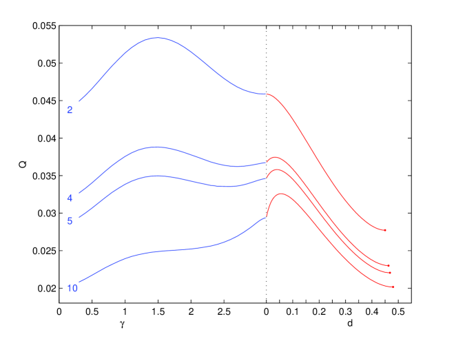
Figure 6: ${\rm max}_{\lambda}Q$ as a function of $\gamma$ for the side-by-side solutions and as a function of $d>0$ for the eccentric solutions at $\beta=2,4,5$ and $10$. The single dot at the right end of each curve corresponds to the concentric case $Q_{c}$. The global flux maximum is a side-by-side solution for $\beta\leq 4.60$ and an eccentric solution for $\beta\geq 4.60$.

Figure 7: Maximal flux side-by-side solutions for $\beta=1$ (top left, $-0.098\leq u\leq-0.098$), $\beta=2$ (top right, $-0.078\leq u\leq 0.063$), $\beta=5$ (bottom left, $-0.058\leq u\leq 0.037$) and $\beta=8$ (bottom right, $-0.047\leq u\leq 0.029$). The contours range from -0.105(dark/red) to 0.105 (light/white) in steps of 0.01 here and throughout figures 5 and 8 to aid comparison.

Figure 8: Maximal flux eccentric core-annular solutions for $\beta=2.5$ (top left, $-0.059\leq u\leq 0.058$ ), $\beta=5$ (top right, $-0.053\leq u\leq 0.044$), $\beta=8$ (bottom left, $-0.051\leq u\leq 0.039$) and $\beta=10,000$ (bottom right, $-0.047\leq u\leq 0.031$). The contours range from -0.105(dark/red) to 0.105 (light/white) in steps of 0.01 here and throughout figures 5 and 7 to aid comparison.

3 Results

There is a special case of the problem which can be solved using known results. When $\beta=1$, the optimal balanced flow of fluid 1 must mirror that in fluid 2. In particular, $\lambda=0$, $\Gamma$ is the diameter $x=0$ and $u=0$ on $\Gamma$. The problems for either fluid then decouple into single phase pressure-driven flow in a ‘half’-cylinder (semicircular cross-section). The flux is $0.07438920$ in our non-dimensional units according to White’s (1991) equation (3-44). This provides an excellent test of the side-by-side computations (see Table 1 which shows 3 significant figure correspondence although there is really 5). Further checks are available between the very different side-by-side and eccentric flow codes (e.g. figure 4 where using $d$ as the abscissa shows at least $C^{1}$ continuity in $\max_{\lambda}Q$ at $\gamma=\pi$ or $d=0$ at $\beta=5$).

3.1 $max_{\lambda}Q$

The $\beta$ value chosen in figure 3 has been purposely chosen to show the presence of flux maxima in the side-by-side solutions and the ($d>0$ or more viscous fluid in the core) eccentric solutions ($Q_{e}$). The complementary eccentric solutions with the less viscous fluid in the core ($\hat{Q}_{e}$) always show monotonic behaviour in which the flux decreases from the $\gamma=0$ side-by-side value down to the concentric core-annular value of $\hat{Q}_{c}$ (leftmost point or most negative $d$). This uninteresting part of the flux spectrum is suppressed in figure 6 to focus on $max_{\lambda}Q$ over $\gamma$ and $d>0$ for $\beta\in[2,10]$ over which all the interesting behaviour occurs. At $\beta=1$, the side-by-side solution with $\gamma=\pi/2$ and $\alpha=\pi/4$ supplies the only flux maximum with both concentric core-annular solutions being global minima as $Q_{c}=\hat{Q}_{c}$. At $\beta\approx 2$, a local maximum starts to appear in the eccentric solutions with $d$ small and positive (see figure 6). At $\beta\approx 4.60$, this ‘eccentric’ maximum becomes the global maximum with the ‘side-by-side’ local maximum disappearing by $\beta\approx 8.2$. Thereafter the sole flux maximum is always an eccentric solution. Figures 7 and 8 show how the maxima change with $\beta$ including an eccentric optimal flux solution at $\beta=10,000$. This confirms that the optimal asymptotic solution has plug flow for the more viscous core. Figure 9 plots the maxima values as a function of $\beta$ highlighting the cross-over point at $\beta\approx 4.60$ (see also Tables 1 and 2). The concentric core-annular flux values for the more viscous fluid in the core $Q_{c}$ and less viscous fluid in the core $\hat{Q}_{c}$ are also shown as a local and global minima respectively.

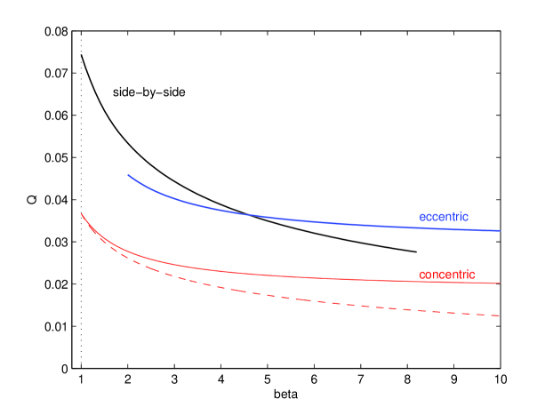
Figure 9: ${\rm max}_{\lambda,\gamma}Q_{s}$ (left upper black curve), ${\rm max}_{\lambda,d}Q_{e}$ (right upper blue curve) and ${\rm max}_{\lambda}Q_{c}$ (lowest solid red curve) compared as a function of $\beta$. The side-by-side maximum disappears for $\beta\gtrsim 8.2$ and the eccentric solution only starts to have a maximum for $\beta\gtrsim 2$. The lowest dashed (red) curve corresponds to $max_{\lambda}\hat{Q}_{c}$, the global minimum of the more viscous fluid encapsulating the less viscous solution.

$\beta$		$\lambda$		$\gamma$		$\alpha$		$Q_{s}$ ($\times 10^{-2}$)
1		0.00		1.57		0.785		7.44
1.5		-0.06		1.52		0.810		6.11
2		-0.10		1.50		0.812		5.34
2.5		-0.13		1.48		0.814		4.82
3		-0.15		1.46		0.813		4.43
3.5		-0.18		1.46		0.809		4.13
4		-0.19		1.47		0.786		3.88
4.5		-0.21		1.47		0.779		3.67
5		-0.22		1.48		0.761		3.50
6		-0.25		1.52		0.721		3.21
7		-0.27		1.58		0.668		2.98
8		-0.28		1.69		0.585		2.79

Table 1: ${\rm max}_{\lambda,\gamma}Q_{s}$ ($Q$ for the side-by-side solution) as a function of $\beta$. The maximum is unique global for $\beta<4.60$ and thereafter is a local maximum until it vanishes for a $\beta$ $\approx 8.2$.

$\beta$		$\lambda$		$\sigma$		$R$		$Q_{e}$ ($\times 10^{-2}$)
2.5		-0.140		-0.393		0.594		4.25
3		-0.155		-0.390		0.590		4.02
3.5		-0.168		-0.387		0.584		3.86
4		-0.180		-0.387		0.582		3.74
4.5		-0.188		-0.386		0.578		3.65
5		-0.198		-0.386		0.574		3.58
6		-0.209		-0.385		0.570		3.47
7		-0.211		-0.382		0.568		3.40
8		-0.222		-0.383		0.565		3.34
9		-0.225		-0.383		0.564		3.29
10		-0.226		-0.381		0.563		3.26
15		-0.246		-0.383		0.555		3.15
20		-0.245		-0.381		0.556		3.10
50		-0.260		-0.381		0.549		3.01
100		-0.260		-0.380		0.551		2.98
200		-0.263		-0.381		0.550		2.96
500		-0.263		-0.3795		0.5485		2.9544
1000		-0.263		-0.3794		0.5476		2.9514
2000		-0.263		-0.3797		0.5473		2.9499
5000		-0.263		-0.3795		0.5479		2.9490
10000		-0.263		-0.3795		0.5479		2.9487
$\infty$		-0.263		-0.3795		0.5480		2.9484

Table 2: ${\rm max}_{\lambda,d}Q_{e}$ ($Q$ for the eccentric solution) as a function of $\beta$. The maximum appears for $\beta\approx 2$, is a local maximum for $2\lesssim\beta<4.60$ and becomes a unique global maximum for $\beta>4.60$.

Figure 10: The coefficients $Q_{\infty}$ and $a_{1}$ (inset) as calculated using the expressions (20) against $\beta$ where $\beta$ and the next smallest value of $\beta$ were used.

3.2 $max_{\lambda}Q$ for $\beta\rightarrow\infty$

At large $\beta$, there is every reason to suspect that the maximal flux possible possesses a simple expansion around its limiting value:

$$max_{\lambda,d}Q_{e}(\beta,\lambda;d)=Q_{\infty}+\frac{a_{1}}{\beta}+\frac{a_{2}}{\beta^{2}}+\ldots$$ (19)

The scalars $Q_{\infty}$ and $a_{1}$ can be estimated as follows

$$Q_{\infty}\approx\frac{\beta_{1}Q(\beta_{1})-\beta_{2}Q(\beta_{2})}{\beta_{1}-\beta_{2}}\qquad a_{1}\approx\frac{\beta_{1}\beta_{2}}{\beta_{2}-\beta_{1}}\biggl{[}Q(\beta_{1})-Q(\beta_{2})\biggr{]}$$ (20)

where $\beta_{1}$ and $\beta_{2}$ have suitably large values. There is good evidence that $Q_{\infty}\approx 2.9484\times 10^{-2}$ and $a_{1}\approx 3.00\times 10^{-2}$ supporting the original assumption: see figure 10. Another check on this value of $Q_{\infty}$ is available by artificially imposing plug flow in the core (e.g. see the lower right solution in figure 8). The matching conditions at $\Gamma$ then simplify to just continuity $u_{1}=u_{2}$ and the condition that the continuation of $u_{1}$ into $A_{2}$ has no logarithmic singularities ($\oint_{\Gamma}{\bf dx.\nabla}u_{1}=0$) which eliminates $\beta$ from the problem. A straightforward search over $\lambda$ and $\sigma$ then reveals the maximum of $Q_{\infty}=2.94844\times 10^{-2}$ at $\lambda=-0.263$ $\sigma=-0.3795$, $R=0.54798$ (and $d=1+\sigma-R=0.0725$).

3.3 $Q(\beta,\lambda)$ for fixed $\lambda$

So far all the results shown have been optimised over the pressure gradient $\lambda$. The presumption is that, in the absence of any explicitly imposed gradient, the flow sets up its own to maximum the volumetric exchange. Figure 11 shows the effect of fixing $\lambda$ on the flux profile at $\beta=5$. The same general trends emerge with one important additional feature highlighted by the $\lambda=-0.5$ curve. Here $\hat{Q}_{c}$ (leftmost point) is approximately the same as $Q_{c}$ (rightmost point). Figure 12 plots the two core-annular flux functions $Q_{c}$ and $\hat{Q}_{c}$ against $\lambda$ to show that the less-viscous core solution flux $\hat{Q}_{c}$ actually exceeds the more-viscous core solution flux $Q_{c}$ for $\lambda\lesssim-0.51$ at $\beta=5$. This threshold pressure gradient montonically decreases as $\beta$ increases to, for example, $\approx-0.89$ at $\beta=100$ (recall $-1<\lambda<1$): see figure 12. Since a $\lambda$ value of -1 translates into a pressure gradient which hydrostatically maintains the denser fluid, the conclusion is that the less-viscous-fluid-in-the-core concentric solution is favoured over its complement for large enough pressure gradients.

Figure 11: The effect of fixing the pressure gradient $\lambda$ at $-0.5$, $0$ and $0.5$ on $Q$ for $\beta=5$. The (black) dashed upper envelope is the result of optimising over $\lambda$ as shown in figure 6.

Figure 12: The concentric core-annular fluxes $Q_{c}(\beta,\lambda)$ and $\hat{Q}_{c}(\beta,\lambda)$ plotted against $\lambda$ for $\beta=5$ (thick solid red and thin solid black respectively) and $\beta=100$ (thick dashed red and thin dashed black respectively). The crossing of the solid lines at $\approx-0.51$ is consistent with figure 11 where $Q_{c}\approx\hat{Q}_{c}$ at $\lambda=-0.5$. The dashed lines cross at $\lambda\approx-0.89$ for a ratio of 100.

4 Discussion

This paper has considered the steady, coaxial flow of two immiscible fluids of different densities and viscosities in a straight vertical cylindrical tube such that their volumetric fluxes balance. Under mild assumptions concerning the interface between the two fluids, the main conclusion is that the flow which optimises the volumetric flux over all possible pressure gradients is always asymmetric. In particular, for viscosity ratios $\lesssim 4.60$ the optimal flow is a side-by-side solution in which each fluid makes contact with a side of the tube and otherwise is an eccentric core-annular solution with the more viscous fluid encapsulated by the less viscous fluid. (In fact, in this latter case, the eccentricity is so marked, that it could look like a side-by-side solution from one direction to the unwary.) The axisymmetric (concentric) core-annular solution in which one fluid encircles the other is surprisingly either a local or global minimiser of the flux. The clear conclusion is that displacing the core of such a flow to one side increases the flux by allowing the outer fluid to ‘bulge’ through the larger gap. This generalises the equivalent observation made for the flow of a single fluid through an eccentric annulus duct (see figure 3-8 on page 127 of White 1991).

The fact that the principle of maximum flux predicts a side-by-side solution at low viscosity ratios does find support in the work of Arakeri et al (2000) and the experiments at Bristol (Beckett et al. 2009). However, Huppert & Hallworth (2007) never mention seeing a side-by-side solution during their low-viscosity-ratio experiments, instead reporting only a steady concentric core-annular flow. More intriguing, however, is that in this core-annular solution, both Huppert & Hallworth (2007) and Beckett et al. (2009) invariably see the lower (less dense) fluid rising along the axis. On the basis that less dense fluids generically are less viscous too, this implies that the less viscous fluid is typically at the core of these observed flows. From the flux perspective, the results presented here show that this globally minimises the flux over all possible pressure gradients! This apparent contradiction is ameliorated somewhat if the pressure gradient set up (or imposed) is towards the maximum possible for exchange (e.g. see figure 12), but nevertheless the core-annular solution still remains a local flux minimiser. The principle of minimum flux (and, coincidentally, minimum dissipation) then appears more useful at large viscosity ratios.

The proper route to resolving this conundrum, of course, is careful consideration of the initial value problem and the stability of the evolving solution to the small disturbances always present. A first step in this direction would be to study the Rayleigh-Taylor instability problem in a cylindrical tube where a fluid of density $\rho_{1}$ and viscosity $\mu_{1}$ fills the half cylinder $z>0$ and a fluid of density $\rho_{2}<\rho_{1}$ and viscosity $\mu_{2}$ occupies $z<0$. Establishing which interfacial deformation mode (axisymmetric or asymmetric) has the largest growth rate as a function of all the parameters present would surely go some way in predicting which type of flow is initiated. However, even this calculation doesn’t seem to have been done yet although Batchelor & Nitsche (1993) come close.

In conclusion, it should be clear that there are some interesting issues surrounding the exchange flow of two fluids in a vertical tube. Even the steady immiscible problem displays an intriguing degeneracy of solution. Focussing on an ad hoc principle of maximum (or minium) flux unfortunately looks to be too simplistic despite its appealing rationale and apparent success in an associated context. This means that there is no avoiding a more formal stability-based approach to explain what is seen in experiments.

5 Acknowledgements

This study was stimulated by ongoing experimental work carried out by the Volcanology group in Earth Sciences at Bristol University (Frances Beckett, Fred Witham, Jerry Phillips and Heidy Mader) with whom I have enjoyed many stimulating discussions. I would also like to thank Carl Dettmann for a reassuring discussion on singular integrals and Diki Porter for sharing his expertise on solving Laplace’s equation in complex geometries.

Appendix A Side-by-side solutions

The geometry of the side-by-side solution is shown in figure 1 to be defined by two parameters: $\gamma$, the (upper) intercept latitude of $\Gamma$ with the duct wall, and $2\alpha$, the angle between $\Gamma$ and duct wall. The coupled Poisson problems (6)-(8) become two Laplace problems by separating off simple inhomogeneous parts as follows

$$u_{1}^{*}=\Phi_{1}+\frac{\lambda+1}{4}(\,x^{2}+y^{2}-1\,),\qquad u_{2}^{*}=\Phi_{2}+\frac{\lambda-1}{4\beta}(\,x^{2}+y^{2}-1\,)$$ (21)

which have been designed to leave the boundary conditions on the duct wall undisturbed. The functions $\Phi_{1}$ and $\Phi_{2}$ then satisfy

$$\nabla^{2}\Phi_{1} = 0\quad{\rm in}\quad A_{1},$$ (22)

$$\nabla^{2}\Phi_{2} = 0\quad{\rm in}\quad A_{2},$$ (23)

with boundary conditions

$$\Phi_{1}=0 {\rm on}\quad x+iy=e^{i\psi}\quad-\gamma\leq\psi\leq\gamma$$ (24)

$$\Phi_{2}=0 {\rm on}\quad x+iy=e^{i\psi}\quad\gamma\leq\psi\leq 2\pi-\gamma$$ (25)

$$\biggl{.}\begin{array}[]{rcr}\Phi_{1}-\Phi_{2}&=&(\frac{\lambda+1}{4}-\frac{\lambda-1}{4\beta})(\,1-x^{2}-y^{2}\,)\\ 2\frac{\partial}{\partial n}(\Phi_{1}-\beta\Phi_{2})&=&\frac{\partial}{\partial n}(\,1-x^{2}-y^{2}\,)\end{array}\biggr{\}}\quad{\rm on}\quad x+iy\in\Gamma\\$$ (26)

Here the interface curve $\Gamma:=\{\,z\,|\,z=x+iy=\sigma+Re^{i\theta}\,;\,|\theta|\leq|\theta_{max}:=\gamma-2\alpha|\,\}$ where

$$\sigma:=-\frac{\sin 2\alpha}{\sin\theta_{max}}\quad\&\quad R:=\frac{\sin\gamma}{\sin\theta_{max}}$$ (27)

are formulae for the centre $(x,y)=(\sigma,0)$ and radius of curvature respectively valid for any pair $0\leq 2\alpha,\gamma\leq\pi$. (The singular case $\gamma=2\alpha$ where $R\rightarrow\infty$ so that $\Gamma$ is a straight line cannot be formally handled but is never a practical problem.)

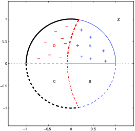
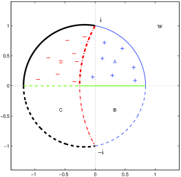
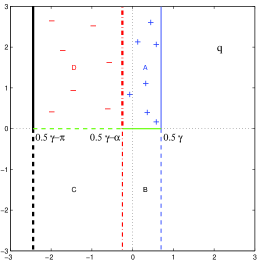
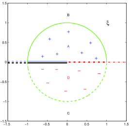
Figure 13: The composite conformal mapping from $z$ to $\xi$. The interface curve $\Gamma$ meets the duct wall at $e^{\pm i\gamma}$ in the $z$-plane, which are moved to $\pm i$ in the $w$-plane, and then to $\pm i\infty$ in the $q$-plane. Two separate transformations then map the strip $\mbox{$\frac{1}{2}$}\gamma-\alpha\leq Re(q)\leq\mbox{$\frac{1}{2}$}\gamma$ onto the upper half plane and the strip $\mbox{$\frac{1}{2}$}\gamma-\pi\leq Re(q)\leq\mbox{$\frac{1}{2}$}\gamma-\alpha$ onto the lower half plane. In both cases, $Im(q)>0$ in mapped inside the appropriate unit semicircle in the $\xi$-plane.

The solution strategy is to transform regions $A_{1}$ and $A_{2}$ into the upper and lower half planes respectively via conformal tranformations where an explicit solution can then be deduced by Poisson’s integral formula. Three simple transformations prove sufficient, the first is

$$w:=\frac{z-\cos\gamma}{\sin\gamma}$$ (28)

which rescales the duct so that its radius becomes $1/\sin\gamma$ and the 2 contact points of $\Gamma$ with the duct wall $e^{\pm i\gamma}$ move to $\pm i$ (other noteworthy images are: $0\rightarrow-\cot\gamma$, $1\rightarrow\sin\gamma/(1+\cos\gamma)$, $-1\rightarrow-\sin\gamma/(1-\cos\gamma)$ ; see Figure 2). A second transformation

$$q=r+is:=\tan^{-1}\,w\qquad\qquad r,s\in\Re e$$ (29)

converts all the circular arcs into straight lines parallel to the imaginary axis in the complex $q$ plane. To see this, consider the transformation in reverse

$$w=\tan q=-i\frac{e^{2iq}-1}{e^{2iq}+1}$$ (30)

and decompose this transformation into its 3 components. A strip $\mbox{$\frac{1}{2}$}\gamma-\alpha\leq r\leq\mbox{$\frac{1}{2}$}\gamma$ with $0<\alpha\leq\pi$ is rotated through $\pi/2$ by $q\rightarrow iq$. Doubling and exponentiating $q\rightarrow iq\rightarrow e^{2iq}$ then tranforms the strip into the interior of a wedge centred at the origin with sides of argument $\gamma-2\alpha$ and $\gamma$. Finally the Möbius transformation $q\rightarrow iq\rightarrow e^{2iq}\rightarrow-i(e^{2iq}-1)/(e^{2iq}+1)$ converts the wedge sides into circular arcs joining the points $w=\pm i$ and the wedge interior into a circular lune with angle $2\alpha$ (see Figure 2 and pages 205-207 of Marushevich 1965). The conformal transformation (29) is undoubtedly not the only one which would do the job (e.g. Vlasov 1986) but is particularly nice since it can used to treat both ‘lunes’ together: $A_{1}$ maps to the strip $\mbox{$\frac{1}{2}$}\gamma-\alpha\leq r\leq\mbox{$\frac{1}{2}$}\gamma$ and $A_{2}$ maps into the strip $\mbox{$\frac{1}{2}$}\gamma-\mbox{$\frac{1}{2}$}\pi\leq r\leq\mbox{$\frac{1}{2}$}\gamma-\alpha$ in the $q$-plane. The intersection $A_{1}\cap A_{2}=\Gamma$ is then the line $\Re e(q)=r=\mbox{$\frac{1}{2}$}\gamma-\alpha$.

The final transformation does, however, need tailoring to each domain separately as follows

$$\xi=\xi_{1}(q) := e^{i\pi(2q-\gamma+2\alpha)/2\alpha}\qquad\hskip 17.07182ptq\,\in\,A_{1}$$ (31)

$$\xi=\xi_{2}(q) := e^{i\pi(2q-\gamma+2\alpha)/(\pi-2\alpha)}\qquad q\,\in\,A_{2}$$ (32)

so that the final composition transformations are

$$\xi_{1}(z) := \exp\biggl{(}\frac{i\pi}{\alpha}[\tan^{-1}w(z)-\mbox{$\frac{1}{2}$}\gamma+\alpha]\biggr{)},$$ (33)

$$\xi_{2}(z) := \exp\biggl{(}\frac{i\pi}{\mbox{$\frac{1}{2}$}\pi-\alpha}[\tan^{-1}w(z)-\mbox{$\frac{1}{2}$}\gamma+\alpha]\biggr{)}$$ (34)

where

$$w(z)=\frac{z-\cos\gamma}{\sin\gamma}=\frac{e^{i\theta}-\cos(2\alpha-\gamma)}{\sin(\gamma-2\alpha)}.$$ (35)

The image of $A_{1}/A_{2}$ is designed as the upper/lower half $\xi$-plane and $\Gamma$ remains a shared boundary (see Figure 2). If we define $\xi=\zeta+i\eta$ and $\overline{\Phi}_{i}(\,\zeta(x,y),\eta(x,y)\,):=\Phi_{i}(x,y)$ ($i=1,2$), the solutions for $\overline{\Phi}_{1}$ and $\overline{\Phi}_{2}$ are then available via Poisson’s integral formula for the half plane

$$\overline{\Phi}_{1}(\zeta,\eta) = \quad\frac{1}{\pi}\int^{\infty}_{-\infty}\frac{\eta\overline{\Phi}_{1}(t,0)}{(\zeta-t)^{2}+\eta^{2}}\,dt$$ (36)

$$\overline{\Phi}_{2}(\zeta,\eta) = -\frac{1}{\pi}\int^{\infty}_{-\infty}\frac{\eta\overline{\Phi}_{2}(t,0)}{(\zeta-t)^{2}+\eta^{2}}\,dt$$ (37)

The conditions (24) and (25) indicate that $\overline{\Phi}_{1}$ and $\overline{\Phi}_{2}$ are only non-zero on the image of $\Gamma$ which is the positive real axis ($t\geq 0$) in the $\xi$-plane. The problem now boils down to determining the function $f(z):=u^{*}_{1}=u^{*}_{2}$ on $\Gamma$ such that the stress matching condition (see (8) on $\Gamma$ holds. Applying this condition is slightly non-trivial because the integrals (36) and (37) are formally singular for $\xi=\zeta+i\eta$ on $\Gamma$. They have well-defined (Cauchy principal) values by continuity with surrounding values of $\xi$ but taking normal derivatives of these integrals and subsequently computing them, nevertheless, requires due care. Consider the normal ($\eta$) derivative of $\overline{\Phi}_{1}$ on $\Gamma$ ($\eta=0$), for example. It is straightforward to show

$$\overline{\Phi}_{1,\eta}(\zeta,\eta)=\quad\frac{1}{\pi}\int^{\infty}_{-\infty}\overline{\Phi}_{1}(t,0)\frac{\partial}{\partial t}\left[\frac{\zeta-t}{(\zeta-t)^{2}+\eta^{2}}\right]\,dt.$$ (38)

and, after integration by parts, then

$$\overline{\Phi}_{1,\eta}(\zeta,0)=\frac{1}{\pi}\int^{\infty}_{-\infty}\frac{\overline{\Phi}_{1,\zeta}(t,0)}{t-\zeta}\,dt=\frac{1}{\pi}\int^{\infty}_{-\infty}\frac{\overline{\Phi}_{1,\zeta}(t,0)-\overline{\Phi}_{1,\zeta}(\zeta,0)}{t-\zeta}\,dt$$ (39)

since the Cauchy principal value of $\int^{\infty}_{-\infty}1/(t-\zeta)dt$ is zero. The last integral on the right hand side of (39) is now regular. The symmetry of the velocity fields under $y\rightarrow-y$ in the $z$-plane can then be invoked to make the integration range finite. This reflectional symmetry carries over to the $\xi$-plane as the symmetry $\overline{\Phi}_{i}(1/t,0)=\overline{\Phi}_{i}(t,0)$ ($i=1,2$) allowing, for example, (36) to be simplified to

$$\overline{\Phi}_{1}(\zeta,\eta)=\frac{\eta}{\pi}\int^{1}_{0}\overline{\Phi}_{1}(t,0)\biggl{[}\frac{1}{(\zeta-t)^{2}+\eta^{2}}+\frac{1}{(t\zeta-1)^{2}+t^{2}\eta^{2}}\biggr{]}\,dt.$$ (40)

and (39) to

$$\overline{\Phi}_{1,\eta}(\zeta,0)=\frac{1}{\pi}\int^{1}_{0}\biggl{[}\,\frac{\overline{\Phi}_{1,\zeta}(t,0)-\overline{\Phi}_{1,\zeta}(\zeta,0)}{t-\zeta}+\frac{t\overline{\Phi}_{1,\zeta}(t,0)}{\zeta t-1}\biggr{]}\,dt+\frac{\overline{\Phi}_{1,\zeta}(\zeta,0)}{\pi}\log\left(\frac{1-\zeta}{\zeta}\right).$$ (41)

These are the integral representations (along with the equivalent ones for $\overline{\Phi}_{2}$) used to impose the matching conditions and calculate the flow solution.

In the matching process, the first step in determining $f$ is to construct a global representation, $f(\theta)=\sum^{N}_{n=1}c_{n}\Psi_{n}(\theta)$, using $\theta$ to parametrise $\Gamma$, $c_{n}$ as the expansion constants and the basis functions

$$\Psi_{n}(\theta):=T_{2n}(\theta/\theta_{max})-T_{2n-2}(\theta/\theta_{max}).$$ (42)

These are defined in terms of Chebyshev polynomials $T_{n}(\theta):=\cos(n\cos^{-1}\theta)$ with each designed to mirror the properties of $f$: $f(\pm\theta_{max})=0$ and $df/d\theta|_{\theta=0}=0$ by the $y-$reflectional symmetry. This symmetry also means that the matching condition needs only to be applied (via collocation at the $N$ positive zeros of $T_{2N+1}$) over the upper half of $\Gamma$. It is tempting to carry out this procedure directly in the $\xi-$plane using the representation (41) and the sister integral for $\overline{\Phi}_{2,\eta}$. However, this proves inaccurate because both have an integrable singularity at $t=0$ ($\theta=\pm\theta_{max}$). This causes loss of accuracy through two separate effects: a) the integrand has a singular derivative at $t=0$ so numerical quadrature is inefficient and b) the collocation points sparsely populate the neighbourhood of $t=0$ at extreme choices of $\alpha$ ($\rightarrow 0$ or $\pi/2$) so the matching is not well imposed and convergence fails short of usual spectral (exponential) accuracy. Instead, the integral representations must be transformed to the physical $z-$plane and matching carried out there.

The velocity profile along $\Gamma$ is always smooth and typically only $N=20$ or $30$ is needed to see spectral drop off of 4-5 orders of magnitude. The limits $\alpha\rightarrow\pi/2$ and $\alpha\rightarrow 0$, however, have to be treated carefully. For example, when $\alpha\geq 0.2$ ($\approx 10^{o}$) only a 100-panel Simpson quadrature is needed to accurately calculate the integrals along $\Gamma$ but this must be increased dramatically as $\alpha\rightarrow 0$ due to the extreme behaviour of the $z=z(\xi)$ transformation in this limit (e.g. $10^{4}$ panels proved sufficient for $\alpha=O(0.001)$). Once the solution is obtained, the fluxes $Q_{1}$ and $Q_{2}$ are calculated using Simpson’s rule with typically $20-40$ panels. This is the most costly part of the process as essentially a triple integral is being evaluated. Simple bisection in $\alpha$ is used to find a ‘balanced’ flux state where $Q_{1}+Q_{2}=0$ for given $\beta$, $\lambda$ and $\gamma$.

As a final comment, it’s worth remarking that the transformation $q=q(z)$ (see the third subplot in figure 13) achieves a separation of variables in the problem (the boundaries are contours of constant $r=Re(q)$). A solution could therefore be developed by separation of variables after a Fourier transform (in $s$) is taken of the inhomogeneity in the matching condition. The full procedure, however, boils down to essentially the same problem of evaluating a triple integral albeit in this case the innermost one for $u$ is an inverse Fourier transform and hence over a semi-infinite interval.

Appendix B Eccentric solutions

The ‘eccentric’ solution has one fluid completely encapsulated by the other. For sake of argument, we describe the solution strategy for $A_{2}$ in $A_{1}$. The radius $R$ and centre $(\sigma,0)$ (with $\sigma<0$) define the geometry uniquely up to an arbitrary rotation around the duct axis and any reflection about a diameter neither of which, of course, affect the flux. The interface curve $\Gamma$ is then

$$\Gamma:=\{\,z\,|\,z=x+iy=\sigma+Re^{i\theta}\,;\,-\pi<\theta\leq\pi\,\}$$ (43)

which smoothly connects to the formula for $\Gamma$ in the side-by-side solution (formally, $R$ is +/$-$ve if $\Gamma$ is convex/concave as viewed from $x=-\infty$: see the definition (27) ). The problem (6)$-$(8) is solved by conformally mapping the geometry of eccentric circles into one of concentric circles using a bilinear transformation $\xi=\xi(z)$. This is constructed by selecting a common pair of real inverse points $(\kappa,0)$ and $(\nu,0)$ for $\Gamma$ and the duct wall $|z|=1$ (so $|\kappa\nu|=1$ and $|\kappa-\sigma||\nu-\sigma|=R^{2}$) which ensures that the transformation

$$\xi:=\frac{z-\kappa}{z-\nu}$$ (44)

maps the two circles $|z|=1$ and $\Gamma$ into concentric circles of radii (respectively)

$$\varpi_{1}:=\frac{1-\kappa}{1-\nu}\quad\&\quad\varpi_{2}:=\frac{R+\sigma-\kappa}{R+\sigma-\nu}$$ (45)

where

$$\left.\begin{array}[]{c}\kappa\\ \nu\end{array}\right\}:=\frac{\pm(1+\sigma^{2}-R^{2})-\sqrt{(1+\sigma^{2}-R^{2})^{2}-4\sigma^{2}}}{2\sigma}$$ (46)

(so $\nu<-1$). In the $\xi=\varpi e^{i\phi}$ plane, the solution is found standardly using the expansions

$$u_{1}=\sum^{N}_{n=1}A_{n}\left(\varpi^{n}-\frac{\varpi_{1}^{2n}}{\varpi^{n}}\right)\cos n\phi+A_{0}\log(\varpi/\varpi_{1})+\frac{\lambda+1}{4}(|z|^{2}-1),$$

$$u_{2}=\sum^{N}_{n=0}B_{n}\varpi^{n}\cos n\phi+\frac{\lambda-1}{4\beta}|z|^{2}$$

which incorporate the boundary condition at $|z|=1$ ($\varpi=\varpi_{1}$) and the $y-$symmetry ($\phi\rightarrow-\phi$) of the problem. The Fourier series in $\phi$ of $|z|=|\nu\xi-\kappa|/|\xi-1|$ and $\partial|z|/\partial\varpi$ on $\Gamma$ need to be evaluated to apply the remaining matching conditions. This is done routinely using Simpson’s rule with 200 panels when $N=100$. In the limiting situations of $\sigma-R\rightarrow-1$ ($\Gamma$ approaching the duct wall) and $\sigma\rightarrow 0$ (approaching concentricity), these numbers are doubled to 400 and $N=200$ to maintain at worst $10^{-10}$ least square error in either matching condition. Calculation of the fluxes in $A_{1}$ and $A_{2}$ is again by 2D Simpson’s rule using 100-200 panels per direction and simple bisection is used in $R$ used to identify where $Q_{1}+Q_{2}=0$ for given $\beta$, $\lambda$ and $1+\sigma-R$ ($1+\sigma-R$ is fixed rather than $\sigma$ to avoid the complication of multiple solutions).

References

- Arakeri, Avila, Dada and Tovar (2000) Arakeri, J.H., Avila, F.E., Dada, J.M. & Tovar, R.O. 2000 Convection in a long vertical tube due to unstable stratification- A new type of turbulent flow? Current Science 79, 859-866.
- Batchelor & Nitsche (1993) Batchelor, G.K. & Nitsche, J.M. 1993 Instability of stratified fluid in a vertical cylinder. J. Fluid Mech. 252, 419-448.
- Beckett et al. (2009) Beckett, F., Witham, F., Phillips, J.C. & Mader, H. private communication concerning experiments curently being carried out in the Department of Earth Sciences, University of Bristol - preprint coming.
- Charles and Redberger (1961) Charles, M.E. & Redberger, R.J. 1961 The reduction of pressure gradients in oil pipelines by the addition of water. Numerical analysis of stratified flows Can. J. Chem. Engng 40, 70-75.
- Frigaard & Scherzer (1998) Frigaard, I.A. & Scherzer, O. 1998 Uniaxial exchange flows of Bingham fluids in a cylindrical duct IMA J. App. Math. 61, 237-266.
- Hasson, Mann & Nir (1970) Hasson, D., Mann, U. & Nir, A. 1970 Annular flow of two immiscible liquids. I. Mechanisms. Can. J. Chem. Engng. 48, 514.
- Huppert & Hallworth (2007) Huppert, H.E. & Hallworth, M.A. 2007 Bi-directional flows in constrained systems J. Fluid Mech. 578, 95-112.
- Joseph, Renardy & Renardy (1984) Joseph, D.D., Renardy, M. & Renardy, Y. 1984 Instability of the flow of two immiscible liquids with different viscosities in a pipe. J. Fluid Mech. 14, 309-317.
- Joseph, Nguyen and Beavers (1984) Joseph, D.D., Nguyen, K. & Beavers, G.S. 1984 Non-uniqueness and stability of the configuration of flow of immiscible fluids with different viscosities. J. Fluid Mech. 14, 319-345.
- (10) Joseph, D.D., Bai, R., Chen, K.P. & Renardy, Y.Y. 1997 Core-annular flows Ann. Rev. Fluid Mech. 29, 65-90.
- Lee and White (1974) Lee, B.L. & White, J.L. 1974 An experimentalstidy of rheological properties of polymer melts in laminar shear flow and of interface defomration and its mechanisms in two-phase stratified flow. Trans. Soc. Rheol. 18, 467.
- Maclean (1973) Maclean, D.L. 1973 A theoretical analysis of bicomponent flow and the problem of interface shape Trans. Soc. Rheol. 17, 385.
- Markushevich (1965) Markuskevich, A. I. 1965 Theory of Functions of a Complex Variable, vol 1 Prentice-Hall, Inc. Englewood Cliffs, New Jersey (p205-207)
- Minagawa and White (1975) Minagawa, N. & White, J.L. 1975 Coextrusion of unfilled and Ti02-filled polyethylene: influence of viscosity and die cross-section on interface shape. Polymer Engng Sci. 15, 825.
- Moyers-Gonzalez & Frigaard (2004) Moyers-Gonzalez, M.A. & Frigaard, I.A. 2004 Numerical solution of duct flows of multiple visco-plastic fluids J. Non-Newtonian Fluid Mech. 122, 227-241.
- Seon et al (2007) Seon, T, Znaien, J., Salin, D., Hulin, J.P., Hinch, E.J. & Perrin, B. 2007 Transient buoyany-driven front dynamics in nearly horizontal tubes Phys. Fluids 19, 123603
- Southern and Ballman (1973) Southern, J.H. & Ballman, R.L. 1973 Stratified bicomponent flow of polymer melts in a tube Appl. Polymer Symp. 20, 175-189.
- Taghavi (2009) Taghavi, S.M., Seon, T., Martinez, D.M. & Frigaard, I.A. 2009 Buoyancy-dominated displacement flows in near-horizontal channels: the viscous limit J. Fluid Mech. 639, 1-35.
- Vlasov (1986) Vlasov, V.I. 1986 Solution of a Dirichlet problem in a crescent-shaped domain J. Eng. Phys. & Thermophys. 50, 741-747.
- White (1991) White, F. M. Viscous Fluid Flow McGraw-Hill (p124)
- Williams (1975) Williams, M.C. 1975 Migration of two liquid phases in capillary extrusion: an energy interpretation AIChE. J. 21, 1204.
- Yu and Sparrow (1967) Yu, H.S. & Sparrow, E.M. 1967 Straified laminar flow in ducts of arbitrary shape AIChE. J. 13, 10.
- Znaien et al (2009) Znaien, J., Hallez, Y., Moisy, F., Magnaudet, J., Hullin, J.P., Salin, D. & Hinch, E.J. 2009 Experimental and numerical investigations of flow structure and momentum transport in a turbulent buoyancy-driven flow inside a tilted tube. Phys. Fluids 21, 115102.