A Non-Disordered Glassy Model with a Tunable Interaction Range

Abstract

We introduce a non-disordered lattice spin model, based on the principle of minimizing spin-spin correlations up to a (tunable) distance $R$. The model can be defined in any spatial dimension $D$, but already for $D=1$ and small values of $R$ (e.g. $R=5$) the model shows the properties of a glassy system: deep and well separated energy minima, very slow relaxation dynamics, aging and non-trivial fluctuation-dissipation ratio.

In a supercooled liquid the viscosity increases abruptly by several order of magnitude in a narrow temperature range, and eventually undergoes a dynamical arrest, that can be observed on any accessible time scale: this is the essence of a fascinating physical phenomenon, the so called “dynamical glass transition”. A vast scientific literature has been dedicated to its study: see CavagnaReview ; KobReview for interesting reviews on the subject. A theoretical understanding of this effect must be based on a reliable modeling of the underlying material: ideally one would like to have at hand very simple models that reproduce the main features of glass-former liquids. From the point of view of a numerical approach, off-lattice simulations are extremely costly in term of computational resources: because of that lattice models where each node of the interacting network contains some degrees of freedom (a binary spin variable in the simplest case) play an important role.

An analytic approach needs some reasonable approximation: mode coupling theory CavagnaReview ; KobReview , for example, helps to shed some light on the problem. At the mean-field level, and more precisely on a fully connected lattice, the solution of the disordered $p$-spin model GM is now very well understood KTW , and it turns out to be equivalent to the mode-coupling theory (based on systems where the Hamiltonian does not include quenched disorder). The main prediction of these mean-field theories is that below the dynamical glass transition $T_{g}$, which is higher than the thermodynamical critical point $T_{k}$, the relaxation dynamics is not able to bring the system to equilibrium in any sub-exponential time (in the system size). Consequently the system relaxes to the so-called threshold energy, which is higher than the equilibrium energy, and the off-equilibrium dynamics shows aging on any measurable time scale . During the aging dynamics the fluctuation-dissipation ratio is different from the one expected in equilibrium, and its behavior presents peculiar and distinctive features.

The mean field scenario is well characterized and well understood, but it is still unclear how to adapt it to real systems. In finite dimensional systems the lifetime of metastable states is limited: eventually, during the aging dynamics, a bubble of the equilibrium state will nucleate and will grow up to the system size. Nonetheless the time for nucleating and growing the equilibrium phase may be extremely large, especially close to a critical point. Moreover the Hamiltonian of a real glass-former does not contain any quenched disorder: this is a crucial difference from the $p$-spin model. The frustration, which is the main ingredient for the slow relaxation, is self-induced by the relaxation dynamics: a realistic model of a glassy system should contain no quenched disorder.

The “kinematic models” RS are glassy models with no quenched disorder, where the evolution is governed by a specific dynamical rule, but it does not correspond to a relaxation on a well-defined energy landscape: they are interesting but they cannot undergo a true thermodynamical phase transition, and we will not consider them in the following.

Not so many “Hamiltonian glassy models” without quenched disorder are available. Shore, Holzer and Sethna HSS92 introduced and analyzed a model with a competition in the interaction, and a tiling $2D$ model. Newman and Moore NM99 have discussed a $2D$ model with a triangle $3$-spin interaction, that can be solved exactly: it does not show a sharp glass transition but undergoes a severe slowing down. Biroli and Mézard BM02 defined a very simple lattice glassy model, where the legal positions of the particles are restricted by hard “density constraints”: the model is versatile, since it does not depend on the detailed feature of the underlying lattice, but its energy landscape is somehow drastic, in the sense that a configuration is either legal ($E=0$) or forbidden ($E=\infty$). Cavagna, Giardina and Grigera CGG03 have discussed a $2D$ model based again on competing interactions (respectively with $4$ and $5$ spins). It is clear that enlarging this collection would be appropriate: some of these interesting models are indeed strictly two dimensional or depend on the detailed lattice structure. In some other cases one can observe a very slow domain growth, but once the time is appropriately rescaled the growth process does not differ qualitatively from the dynamics of the pure Ising model.

In this note we define and analyze a new non-disordered glassy model, that can be defined on any lattice structure, in any dimension, and is based on a simple physical principle: the minimization of correlations. Our model is also, following the route of its mean field predecessor, a good candidate for providing coding for an effective and secure communication.

We are inspired from the Bernasconi mean field model GO ; BE , where one is interested in finding the assignment to $N$ Ising spins defined on a linear lattice that minimizes the sum $\mathcal{H}_{\text{B}}\equiv\frac{1}{N-1}\sum_{d=1}^{N-1}\left(\sum_{j=0}^{N-d-1}\sigma_{j}\sigma_{j+d}\right)^{2}$ of the squared spin-spin correlations. We have used here open boundary conditions, but the Bernasconi model, like our model, is also interesting when defined with periodic boundary conditions. The Bernasconi model has a very rough energy landscape BOME ; MPR1 , with deep minima separated by extensive energy barriers, making the search for global minima (low auto-correlation binary sequences) a very difficult task. The theoretical analysis of this model predicts a thermodynamical phase transition with one step of replica symmetry breaking (1RSB), in the same universality class of the $p$-spin model, preceded by a dynamical glass transition. Extensive numerical simulations have shown that the energy relaxation stops before reaching the ground state (GS) energy, and the aging regime persist for extremely long times. For these reasons the Bernasconi model is the perfect prototype of a glassy mean field model.

We define our model by adopting the principle of minimizing spin-spin correlation functions, but using an interaction that is local in space: in $D$ dimensions the Hamiltonian reads

$$\mathcal{H}_{D}=\mathcal{N}_{N,R}\sum_{\vec{x}\in\Lambda}\left[\sum_{d=1}^{\text{max }d\text{ in }\mathcal{R}(\vec{x})}\left(\sum^{\text{couples in }\mathcal{R}(\vec{x})}_{\text{ at distance }d}\sigma_{j}\sigma_{k}\right)^{2}\right]$$ (1)

where $\Lambda\subset\mathbb{Z}^{D}$ is a finite volume of cardinality $N$, $\mathcal{R}(\vec{x})$ is a hypercube of size $R^{D}$ (or its intersection with $\Lambda$ if open boundary conditions are used) centered around site $\vec{x}$, and $\mathcal{N}_{N,R}$ is a normalization constant that guarantees good $R\to\infty$ and $N\to\infty$ limits. The sum over $d$ is for distances going from one up to the maximum distance contained in $\mathcal{R}(\vec{x})$. One can also define the model by only considering correlations on the $D$ axis: from the point of view of computational cost this is a far better choice.

With eq. (1) we are aiming at minimizing correlations in blocks of linear size $R$. Since correlations at short distances are typically the strongest, the overall effect is to have low-energy configurations showing very weak correlations on all length scales. This seems to us a very solid first principle to build a glassy model: glass-formers show no long range order in the two-point correlation functions and we are somehow enforcing this condition in the Hamiltonian. The tunable interaction range $R$ is a novel and very useful feature of our model. The $R\to\infty$ limit gives back the Bernasconi model in $D=1$, and for $D>1$ provides new and potentially interesting mean-field models. As for the Bernasconi model here we can get a good basis towards effective coding: the introduction of new, free parameters ($D$ and $R$) that are unknown to the observer could be of further help.

Let us look in better detail to the $D=1$ version of the model with open boundary conditions. The Hamiltonian reads

$$\mathcal{H}_{1}=\frac{N}{N-R+1}\sum_{i=0}^{N-R}\frac{1}{R(R-1)}\sum_{d=1}^{R-1}C(d,i,R)^{2}\;,$$ (2)

where $C(d,i,R)\equiv\sum_{j=i}^{i+R-1-d}\sigma_{j}\sigma_{j+d}$, and $R$ is the tunable interaction range. We will show, for example, that the $R=5$ model presents to a very large extent the glassy phenomenology we have described above (as opposed, for example, to the $R=6$ model). This makes clear that already the $D=1$ case, where a thermodynamical transition is forbidden, is very interesting for the physics of structural glasses.

Finding and analyzing low energy configurations is our first task. For $R=N$ (the Bernasconi model) finding a GS is difficult in practice and requires a time growing exponentially with $N$. For finite $R$ the model can be solved in a time of order $O(N2^{2(R-3)})$ by transfer matrix methods, using the variables $\tau_{i}\equiv\sigma_{i-1}\sigma_{i+1}$.

We have computed GS and first excited states for any $N\leq 52$ and $R$ from $3$ to $6$ (for some selected $N$ values we have also analyzed $R$ values going up to $N$), using exact algorithms. For a given couple $N,R$ we have determined all exact GS using a clever exhaustive enumeration scheme called branch-and-bound (b&b). In b&b, the problem is solved using recursion. In a branching step, one of the variables $\sigma_{i}$ is chosen, and it is eliminated by creating two subproblems in one of which $\sigma_{i}=+1$, and in the other $\sigma_{i}=-1$. The latter are solved recursively. A subproblem is solved by determining upper and lower bounds on its optimum solution value. The energy value $E^{ub}$ of the best known configurations serves as upper bound. The latter are updated whenever configurations with energy $E^{ub}$ or better could be determined. If a subproblem’s lower bound attains a higher value than $E^{ub}$, no configuration with lower energy can be contained in it. Thus, it can be excluded from further consideration (fathoming step). For designing a practically effective algorithm, it is crucial to employ a strong lower bound with which subproblems can be fathomed early, keeping their total number reasonably small. For additionally determining all excited states with value at most $x\%$ away from optimality, we fathom a node only if its lower bound is worse than $(1.0+\frac{x}{100})E^{0}$, being $E^{0}$ the exact GS energy (determined in an earlier run of b&b). Mertens Me96 has developed a b&b approach for determining exact GS for the model restricted to $R=N$. He could solve the problem up to $N=60$, which marks the world record. Following Me96 , we first narrow the search space by exploiting the fact that if the configuration $\sigma_{1}\ldots\sigma_{n}$ is a GS also its reversal $\sigma_{n}\ldots\sigma_{1}$ is a GS. The same is true when each odd spin and/or each even spin is multiplied by $-1$. We restrict ourselves to representatives of these symmetry classes.

A lower bound on $\mathcal{H}_{1}$ is given by minimizing each $C(d,i,R)^{2}$ independently. We briefly sketch how we estimate the value of such a minimum. In a subproblem, several spins might be fixed, all other spins are yet free. The already fixed parts give some contribution, say $Z$. We look at all partial sequences of free spins at distance $d$, i.e., $\sigma_{i+kd},\sigma_{i+(k+1)d},\ldots,\sigma_{i+ld}$ that are framed by fixed spins. Depending on whether $Z$ is negative or not, the smallest possible value of $C(d,i,R)$ is either achieved when the free spins are all set equal or all alternating. The bound that we calculate from this is stronger than the one presented in Me96 in the sense that we need to enumerate considerably less subproblems. For small and medium $R$ we get better performance if we start branching by fixing the spins in the middle of the sequence, expanding towards the boundaries, than if we start branching on the spins along the boundary, moving ‘inwards’.

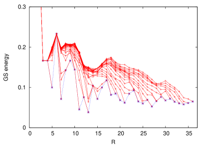
Figure 1: GS energy as a function of $R$, for different $N$ values.

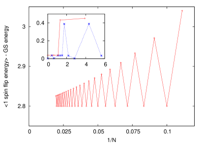
Figure 2: R=5. Average energy of states at one spin flip from the GS. The energy gap in $\mathcal{H}_{1}$ is $4$. In the inset the probability distribution of these energies for $N=50$ (dashed) and $N=51$ (continuous).

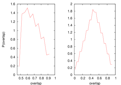
Figure 3: Probability distribution of the overlap among the GS and the first excited states. $N=50$ (left) and $N=51$ (right).

In Fig. 1 we show the GS energy as a function of $R$. Different full lines correspond to different $N$ values (increasing from bottom to top). The lower dashed line joins data points with $R=N$. For $N\gg R$ (upper lines for low $R$ values) the data accumulate on a limiting curve: the thermodynamic model with $R$ fixed is well defined. For $R\leq 12$ we worked out an iterative procedure for computing the GS configurations for any $N$ value. The $N\gg R$ limiting curve has, like the infinite range Bernasconi model, an erratic $R$ dependence, but smoother than in that case.

We have run extensive simulated annealing experiments for $R\leq 13$ (to be better discussed below) and we have identified models where the energy relaxes fast to the GS one, e.g. $R=3,6$, and models showing a very slow relaxation, e.g. $R=5,7$. In the rest of the Letter we focus on the $R=5$ model, which seems the best compromise between very short range interactions and glassiness on quite long time scales .

In Fig. 2 we show the average energy difference $\delta$ of states at one spin flip from the GS as a function of $N^{-1}$. The limit $N\to\infty$ can be estimated very reliably, and is close to $2.8$, i.e. more than ten times the gap (that in these units is equal to $0.2$). In the inset we plot the probability distributions of these energies for $N=50$ and $N=51$: they make clear that the large mean value of $\delta$ comes from a quasi totality of configurations that have energies that are much larger than the GS one. The distributions shown in the inset only depend, for large $N$, on $N$ being odd (where there is a single GS) or even (where there is a $N/2+1$-fold degeneracy of the GS). This is a strong evidence that GS are surrounded by high barrier of the order of several energy gaps. This property is shared also by low energy configurations, and it is what makes the energy landscape somehow golf-course-like.

In Fig. 3 we show the probability of the overlap $q\equiv\frac{1}{N}\sum_{i}\sigma_{i}^{(GS)}\sigma_{i}^{(FIRST)}$ among the GS and the first excited states, for $N=50$ and $N=51$. We consider all first excited states and compute $q$ with the GS that is closest in Hamming distance. The qualitative difference of the two distributions for $q$ smaller than $1/2$ is connected to the fact that the GS is not degenerate for odd values of $N$. These probabilities are peaked at a value of $q$ different from one, and by increasing $N$ the mean value of $q$ stays well below $1$. The number of first excited states very similar to the GS is small; they are typically far from the GS. This is a further hint towards a glassy nature of the system.

We discuss now the finite $T$ properties of the model (mainly for $R=5$). The system size is always $N=10^{6}$. In the main panel of Fig. 4 we show the relative difference $\Delta$ between the system energy and the GS energy during very slow annealing and heating experiments (marked by leftward and rightward arrows respectively) . Temperature values look small, but this depends on the factor $1/(R(R-1))$ used in Eq.(2): the relevant energy scale is the gap, which is $0.2$ for $R=5$. While the $R=6$ model fastly relaxes to the GS energy, the $R=5$ one shows a very slow relaxation: a tentative extrapolation to the adiabatic limit using an inverse power of the running time returns $\Delta\simeq 0.048$, i.e. is roughly 5% above the GS energy. Results from heating experiments look like a crystal melting, although the dependence on the heating rate is strong. For $R=5$ the exact energy is plotted with a dashed line: it is worth noticing the presence at $T\simeq 0.038$ of a secondary peak in $C_{v}$, that seems to enhance hysteresis in temperature cycles.

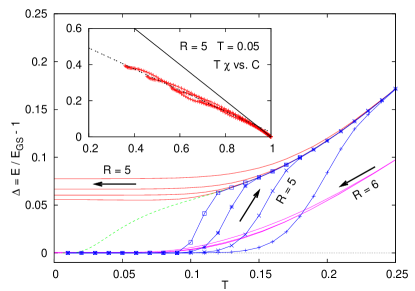
Figure 4: Cooling and heating experiments: for $R=6$ the model fastly relaxes to the GS, while for $R=5$ it has a glassy dynamics. The dashed line is the exact energy for $R=5$. Inset: integrated response versus correlation ($t_{w}$ values as in Fig. 5).

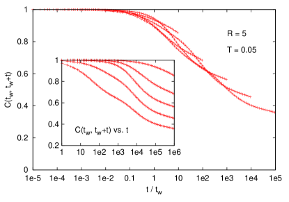
Figure 5: Correlation function $C(t_{w},t_{w}+t)$ as a function of $t$ (inset) and of $t/t_{w}$ (main panel). Values of $t_{w}$ are $10,10^{2},10^{3},10^{4},10^{5}$.

We show in Fig. 5 the two-time autocorrelation function $C(t_{w},t_{w}+t)\equiv N^{-1}\sum_{i}\sigma_{i}(t_{w})\sigma_{i}(t_{w}+t)$ for different values of the waiting time $t_{w}=10,10^{2},10^{3},10^{4},10^{5}$. When plotted as a function of $t$ (inset), the aging behavior is clear, and very similar to the one observed, for example, in a Lennard-Jones mixture KobReview . The oscillations are maybe due to the deterministic nature of the model as in Ref. NM99 . There is a strong dependence of the decay rate on the waiting time $t_{w}$. We show in the main panel how data collapse when plotted versus $t/t_{w}$: again, we have a very good agreement with the behavior observed in glassy systems.

In order to test more quantitatively the out of equilibrium regime, we have also measured the integrated response to an infinitesimal field switched on at time $t_{w}$. We have used the algorithm described in Ref. FedeFDR . We show in the inset of Fig. 4 the usual plot of the integrated response $\chi(t_{w},t_{w}+t)$ versus the autocorrelation $C(t_{w},t_{w}+t)$ parametrically in $t$: in the region where $C$ is not too close to $1$ the data follow a line of slope smaller than $1$ (in absolute value) as for the $p$-spin model and for glass-formers.

We have defined a class of models that are potentially good descriptions of glasses. We have shown that already one of the simplest models of our class, the $D=1$ and $R=5$ model, has glassy properties. We have analyzed the low energy landscape (introducing a new effective bound in the optimization process), and used Monte Carlo dynamics to qualify its finite $T$ behavior. There is much interesting work left, on the mathematical analysis of the model, on the study of different values of $R$ and the Kac limit, and on the $D>1$ problem.

We acknowledge interesting discussions with A. Billoire and S. Franz. We are aware that T. Sarlat, A. Billoire, G. Biroli and J.-P. Bouchaud are studying a local version of the ROM model.

References

- (1) A. Cavagna, Physics Reports 476, 51 (2009).
- (2) W. Kob, Supercooled liquids, the glass transition, and computer simulations, preprint arXiv:cond-mat/0212344.
- (3) D.J. Gross and M. Mezard, Nucl. Phys. B 240, 431 (1984).
- (4) T.R. Kirkpatrick and P.G. Wolynes, Phys. Rev. A 35, 3072 (1987); T.R. Kirkpatrick and D. Thirumalai, Phys. Rev. B 37 5342 (1988).
- (5) F. Ritort and P. Sollich, Advances in Physics 52, 219 (2003).
- (6) J. D. Shore, M. Holzer and J. P. Sethna, Phys. Rev. B 46, 11376 (1992).
- (7) M. E. J. Newman and C. Moore, Phys. Rev. E 60, 5068 (1999).
- (8) G. Biroli and M. Mézard, Phys. Rev. Lett. 88, 025501 (2002).
- (9) A. Cavagna, I. Giardina and T. S. Grigera, J. Chem. Phys. 118, 6974 (2003).
- (10) M. Golay, IEEE Trans. Information Theory 28, 543 (1982).
- (11) J. Bernasconi, J. Physique 48, 559 (1987).
- (12) J. P. Bouchaud and M. Mezard, J. Physique I 4, 1109 (1994).
- (13) E. Marinari, G. Parisi and F. Ritort, J.Phys. A 27, 7615 (1994).
- (14) S. Mertens, J. Phys. A 29, L473 (1996).
- (15) F. Ricci-Tersenghi, Phys. Rev. E 68, 065104 (2003).