Lexical evolution rates by automated stability measure

Abstract

Phylogenetic trees can be reconstructed from the matrix which contains the distances between all pairs of languages in a family. Recently, we proposed a new method which uses normalized Levenshtein distances among words with same meaning and averages on all the items of a given list. Decisions about the number of items in the input lists for language comparison have been debated since the beginning of glottochronology. The point is that words associated to some of the meanings have a rapid lexical evolution. Therefore, a large vocabulary comparison is only apparently more accurate then a smaller one since many of the words do not carry any useful information. In principle, one should find the optimal length of the input lists studying the stability of the different items. In this paper we tackle the problem with an automated methodology only based on our normalized Levenshtein distance. With this approach, the program of an automated reconstruction of languages relationships is completed.

1 Introduction

Glottochronology tries to estimate the time at which languages diverged with the implicit assumption that vocabularies change at a constant average rate. The concept seems to have his roots in the work of the French explorer Dumont D’Urville. He collected comparative words lists of various languages during his voyages around the Astrolabe from 1826 to 1829 and, in his work about the geographical division of the Pacific [3], he introduced the concept of lexical cognates and proposed a method to measure the degree of relation among languages. He used a core vocabulary of 115 basic terms which, impressively, contains all but three the terms of the Swadesh 100-item list. Then, he assigned a distance from 0 to 1 to any pair of words with same meaning and finally he was able to resolve the relationship for any pair of languages. His conclusion is famous: La langue est partout la même.

The method used by modern glottochronology, developed by Morris Swadesh [17] in the 1950s, measures distances from the percentage of shared $cognates$. Recent examples are the studies of Gray and Atkinson [5] and Gray and Jordan [6]. Cognates are words inferred to have a common historical origin, and cognacy decisions are made by trained and experienced linguists. Nevertheless, the task of counting the number of cognate words in a list is far from being trivial and results may vary for different studies. Furthermore, these decisions may imply an enormous working time.

Recently, we proposed a new automated method [15, 13] which has some advantages, the first is that it avoids subjectivity the second is that results can be replicated by other scholars assuming that the database is the same, the third is that no specific linguistic knowledge is requested, and the last, but surely not the least, is that it allows for rapid comparison of a very large number of languages. We applied our method to the Indo-European and the Austronesian groups considering, in both cases, fifty different languages.

In our work, we defined the distance of two languages by considering a normalized Levenshtein distance among words with the same meaning and we averaged on the two hundred words contained in a 200 words list [19]. The normalization, which takes into account word length, plays a crucial role, and no sensible results would have been found without.

Almost at the same time, the above described automated method was used and developed by another large group of scholars [1, 9]. In their work, they used lists of 40 words while we used lists of 200. Their choice was taken according to a careful study of the stability of different words.

Decisions about the number of words in the input lists for languages comparison was debated since the beginning of glottochronology, Swadesh himself switched from 200 words lists to 100 words ones. The point is that a large vocabulary comparison is only apparently more accurate, on the contrary, many of the words do not carry any information on language similarity, and their inclusion in the lists has the only effect of increasing the error noise that may hide the wanted results. In fact, words evolve because of lexical changes, borrowings and replacement at a rate which is not the same for all of them. The speed of lexical evolution, is different for different meanings and it is probably related to the frequency of use of the associated words[12] . Those meanings with a high rate of change turns to be useless to establish relationships among languages. Furthermore the study of words stability has an interest in itself since it may give strong information on the activities which are at the core of the behavior of a social or ethnic group.

The idea of inferring the stability of an item from its similarity in related languages goes back a long way in the lexicostatistical literature[8, 11, 18]. In this paper we tackle this problem with an automated methodology based on normalized Levenshtein distance. For any meaning, and any linguistic group, we are able to find a number which measure its stability (or degree of evolution speed) in a completely objective and reproducible manner. With this approach, the program of an automated reconstruction of languages relationships is completed. This is different from the approach in [1, 9] since they have a combined approach, their lists are chosen according to a stability study which makes use of cognates, and then they reconstruct the languages phylogeny by using Levenshtein distance.

In the next section we define the lexical distance between words and we also sketch our method for computing the time divergence between languages. Section 3 is the core of the paper, there we define the automated stability measures of the meanings and we make some preliminary study concerning distribution and ranking of stability for Indo-European languages. In section 4 we study correlations and Fouldy-Robinson differences associated to lists of different length. We take here the decision about the meanings that should be included in the lists. Conclusions and outlook are in section 5.

2 Definition of distance

We define here the lexical distance between two words which is a variant of the Levenshtein (or edit) distance. The Levenshtein distance is simply the minimum number of insertions, deletions, or substitutions of a single character needed to transform one word into the other. Our definition is taken as the edit distance divided by the number of characters in the longer of the two compared words.

More precisely, given two words $\alpha_{i}$ and $\beta_{j}$ their distance $D(\alpha_{i},\beta_{j})$ is given by

$$D(\alpha_{i},\beta_{j})=\frac{D_{l}(\alpha_{i},\beta_{j})}{L(\alpha_{i},\beta_{j})}$$ (1)

where $D_{l}(\alpha_{i},\beta_{j})$ is the Levenshtein distance between the two words and $L(\alpha_{i},\beta_{j})$ is the number of characters of the longer of the two words $\alpha_{i}$ and $\beta_{j}$. Therefore, the distance can take any value between 0 and 1. Obviously $D(\alpha_{i},\alpha_{i})=0$ .

The normalization is an important novelty and it plays a crucial role; no sensible results can been found without[15, 13].

We use distance between pairs of words, as defined above, to construct the lexical distances of languages. For any pair of languages, the first step is to compute the distance between words corresponding to the same meaning in the Swadesh list. Then, the lexical distance between each languages pair is defined as the average of the distance between all words[15, 13]. As a result we have a number between 0 and 1 which we claim to be the lexical distance between two languages.

Assume that the number of languages is $N$ and the list of words for any language contains $M$ items. Any language in the group is labeled a Greek letter (say $\alpha$) and any word of that language by $\alpha_{i}$ with $1\leq i\leq M$. Then, two words $\alpha_{i}$ and $\beta_{j}$ in the languages $\alpha$ and $\beta$ have the same meaning (they corresponds to the same meaning) if $i=j$.

Then the distance between two languages is

$$D(\alpha,\beta)=\frac{1}{M}\sum_{i}D(\alpha_{i},\beta_{i})$$ (2)

where the sum goes from 1 to $M$. Notice that only pairs of words with same meaning are used in this definition. This number is in the interval [0,1], obviously $D(\alpha,\alpha)=0$.

The results of the analysis is a $N\times N$ upper triangular matrix whose entries are the $N(N-1)$ non trivial lexical distances $D(\alpha,\beta)$ between all pairs in a group. Indeed, our method for computing distances is a very simple operation, that does not need any specific linguistic knowledge and requires a minimum of computing time.

A phylogenetic tree can be constructed from the matrix of lexical distances $D(\alpha,\beta)$, but this gives only the topology of the tree whereas the absolute time scale is missing. Therefore, we perform [15, 13] a logarithmic transformation of lexical distances which is the analogous of the adjusted fundamental formula of glottochronology[16]. In this way we obtain a new $N\times N$ upper triangular matrix whose entries are the divergence times between all pairs of languages. This matrix preserves the topology of the lexical distance matrix but it also contains the information concerning absolute time scales. Then, the phylogenetic tree can be straightforwardly constructed.

In [15, 13] we tested our method constructing the phylogenetic trees of the Indo-European group and of the Austronesian group. In both cases we considered $N=50$ languages. The database[19] that we used in [15, 13] is composed by $M=200$ words for any language.. The main source for the database for the Indo-European group is the file prepared by Dyen et al. in [4]. For the Austronesian group we used as the main source the lists contained in the huge database in [7].

Criticism has been made to our proposal [10] on based on the fact that our reconstructed tree presents some incongruence as for example the early separation of Armenian which is not grouped together with Greek (which, in our tree separate just after Armenian). Nevertheless, the structure of the top of the Indo-European tree is debated and no universally accepted conclusion exists.

In our previous work we have adopted the historically motivated choice of 200 words lists with the meanings proposed by Swadesh. Our aim, in this paper, is to establish in a objective manner the proper length and the composition of the lists. In order to reach this goal we need to separately study the stability of any meaning.

3 Stability of meanings

We take now decisions concerning stability of meanings. Our aim is to obtain an automated procedure, which avoids, also at this level, the use of cognates. For this purpose, it is necessary to obtain a measure of the typical distance of all pairs of words corresponding to a given meaning in a language family. The meaning is indicated by the label $i$ and $\alpha_{i}$ is the corresponding word in the language $\alpha$. Therefore, we define the stability as:

$$S(i)=1-\frac{2}{N(N-1)}\sum_{\alpha>\beta}D(\alpha_{i},\beta_{i})$$ (3)

where the sum goes on all possible $N(N-1)/2$ possible language pairs $\alpha$, $\beta$ in the family using the fact that $D(\alpha_{i},\beta_{i})=D(\beta_{i},\alpha_{i})$.

With this definition, $S(i)$ is inversely proportional to the average of the distances $D(\alpha_{i},\beta_{i})$ and takes a value between 0 and 1. The averaged distance is smaller for those words corresponding to meanings with a lower rate of lexical evolution since they tend to remain more similar in two languages. Therefore, to a larger $S(i)$ corresponds a grater stability.

We computed the $S(i)$ for the 200 meanings of 50 languages of the Indo-European family. To have a first qualitative understanding of the distribution of the $S(i)$ we plot the associated histogram in Fig 1. We can see that there is a fat tail on the right of the histograms indicating that there are some meaning with a quite large stability. This tail is at very variance with a standard Gaussian behavior. The same result are obtained if we consider the Austronesian family instead. We remark that similar plots were computed in [12] were the rates of lexical evolution are obtained by the standard glottochronology approach.

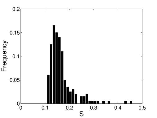
Figure 1: Stability histogram of meanings for Indo-European languages. The fat tail on the right of the histogram indicates that some items have a very large stability.

To understand better the behavior of the stability distribution, we plotted $S(i)$, in decreasing rank, for the 200 meaning in the list. In Fig. 2 are reported the data concerning Indo-European family. At the beginning the stability drops rapidly, then, between the 50th position and the 180th it decreases slowly and almost linearly with rank, finally at the end the stability drops again. We stress again that this behaviour is not Gaussian for which high and low stability part of the curve would be symmetric. The curve is fitted by a straight line in the central part of the data, between position 51 and position 180, in order to highlight the initial and final deviation from the linear behavior. We remark that the qualitative behavior for the Austronesian family is exactly the same.

A preliminary conclusion is that one should surely keep all the meanings with higher information, take at least some of the most stable meanings in the linear part of the curve and exclude completely those meanings with lower information. Nevertheless, at this stage it is difficult to say how many items should be maintained, since this number could be any between 50 and 180.

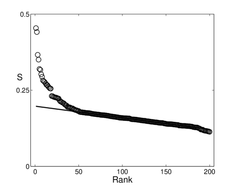
Figure 2: Stability in a decreasing rank for the 200 meanings of the Indo-European languages. At the beginning stability has large values but drops rapidly, then, between the 50th position and the 180th it decreases linearly, finally it drops again. The straight line between position 51 and position 180 underlines the initial and final deviation from the linear behavior.

It is necessary a deeper analysis of the stability to reach a conclusion. Indeed, we need to know what is the minimum number of meaning which allows for a precise computation of distances between languages and, consequently, permits an accurate construction of the phylogenetic tree. In order to reach this goal we need a careful analysis of correlations among distances computed with the whole list and distances computed with shorter lists. It is also necessary to compare the phylogenetic trees by a proper measure, the most natural being the Robinson-Foulds difference.

4 Correlations

As mentioned in the previous section, first of all we need to evaluate the impact of shorter lists on our estimate of the distances between languages. In order to reach this goal, we compute the correlation coefficient $c(n)$ between distances $D(\alpha,\beta)$ obtained by the whole list of 200 items and the distances $D_{n}(\alpha,\beta)$ obtained only by the most $n$ stable items (obviously, $D(\alpha,\beta)$=$D_{200}(\alpha,\beta)$).

The correlation coefficient $c(n)$ is computed in a standard way, using averages over all possible pairs of languages and it takes the value 1 only when there is complete coincidence between $D_{n}(\alpha,\beta)$ and $D(\alpha,\beta)$ . The correlation is plotted in Fig 3 for the Indo-European family. Also in this case similar results are found if the Austronesian family is considered.

From the figure one can observe that the correlation reaches a value larger than $99\%$ with 100 meanings.

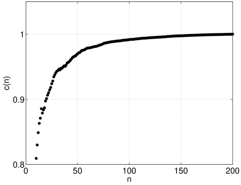
Figure 3: Correlation coefficient $c(n)$ of distances for Indo-European languages. The coefficient $c(n)$ measures the correlation between the distances estimated with $n$ items and the distances estimated with 200 items. $c(n)$ reaches a value larger than $99\%$ at $n=100$.

The problem, is again that our choice for the length of the lists depends on our choice for the minimum excepted correlation coefficient. If we accept $97\%$ we are satisfied by lists of 50 meanings while if we need $99\%$ we have to take lists of 100 meanings.

To resolve this problem we estimated the Robinson-Foulds difference[14] between the trees generated stating from $D_{n}(\alpha,\beta)$ and the tree generated starting from $D(\alpha,\beta)$. The RF difference, which is plotted in Figure 3 for the Indo-European family, measures the degree of similarity between two trees. At lower values correspond trees which are more similar.

As one can see from Fig. 4, the RF difference drops rapidly until $n\sim 100$. Than it remains almost constant for all values greater then $n=100$ (the RF difference is equal to zero when $n=200$ but this is expected since $D_{200}(\alpha,\beta)=D(\alpha,\beta)$) This result says that with 100 meanings one is able to capture all the information regarding languages distance and larger lists produce the same output. In other words, the 100 meanings which have been eliminated carry small, if not vanishing, information.

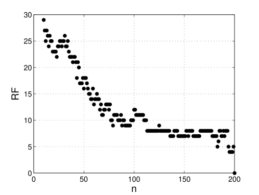
Figure 4: Robinson-Foulds difference between trees of Indo-European languages computed with lists of 200 items and lists of $n$ items. The RF difference measures the degree of similarity between trees. More similar trees have a smaller difference. The RF difference drops rapidly until $n\sim 100$, than it remains almost constant for all greater values of $n$.

The complete list of the most 100 stable terms for the Indo-European group can be found in Table 1. The list is ordered by ranking, and the stability value is written correspondingly to any item.

Table 1: List of the 100 most stable meanings according to the $S(i)$ measure described in the text.

Word	$S(i)$	Word	$S(i)$	Word	$S(i)$	Word	$S(i)$
you	0.45395	three	0.44102	mother	0.36627	not	0.35033
new	0.31961	nose	0.3169	four	0.30226	night	0.29403
two	0.28214	name	0.27962	tooth	0.27677	star	0.27269
salt	0.26792	day	0.26695	grass	0.26231	sea	0.25906
die	0.25602	sun	0.25535	one	0.23093	feather	0.23055
give	0.22864	sit	0.22757	stand	0.22644	meat	0.2261
long	0.22491	five	0.22353	hand	0.22261	short	0.21676
father	0.21319	smoke	0.21213	far	0.20998	worm	0.20846
dry	0.207	scratch	0.20343	person	0.20129	when	0.20011
wind	0.19535	snake	0.19485	sing	0.19434	stone	0.19369
suck	0.19196	mouth	0.19067	dig	0.19052	live	0.18716
root	0.18715	hair	0.18522	smooth	0.18457	water	0.18378
tongue	0.18194	animal	0.1819	year	0.17892	red	0.17815
man	0.17801	tie	0.17789	snow	0.17697	sew	0.17686
there	0.17657	breathe	0.17578	flower	0.17566	mountain	0.17545
fruit	0.17508	bark	0.17502	sand	0.17443	leaf	0.1739
warm	0.17283	green	0.17269	liver	0.17205	hunt	0.17168
sky	0.17156	know	0.17117	bone	0.17056	spit	0.17036
heart	0.17023	pull	0.16984	right	0.1689	we	0.16858
husband	0.16853	foot	0.1683	drink	0.16828	see	0.16764
lie	0.16763	fish	0.16693	woman	0.16656	louse	0.16624
straight	0.16534	yellow	0.16487	sleep	0.1643	black	0.16408
who	0.16351	seed	0.16299	wing	0.16288	cut	0.16245
count	0.16173	thin	0.16156	sharp	0.1611	float	0.16028
fall	0.15968	earth	0.15965	kill	0.15926	burn	0.15918

In conclusion, one has to consider lists with the 100 meaning with higher stability, compute the matrix of lexical distances, transform in the matrix of divergence times and, finally, construct the tree. The elimination of the 100 items with lower stability has the positive effect of reducing the working time necessary for an accurate check of all items and, therefore, reducing errors due to misspelling or inaccurate transliterations. Furthermore, shorter lists allow for comparison of languages whose available vocabulary is small.

5 Discussion and conclusions

In previous works [15, 13] we proposed an automated method for evaluating the distance between languages. Here we propose a method that is also automatic and gives lists of the mosts table meanings. The novelty is that combining [15, 13] with the results presented here everything can be done automatically. Stable meanings, distances, divergence times and phylogenetic trees can be all obtained by using simple objective arguments based on normalized Levenshtein distance.

We do not claim that our combined method produces better results then the standard glottochronology approach, but surely comparable. The advantages of this approach can be summarized here as follows: it avoids subjectivity since all results can be replicated by other scholars assuming that the database is the same; it allows for rapid comparison of a very large number of languages; can be used also for those languages groups for which the use of cognates is very complicated or even impossible. In fact, the only work is to prepare the lists, while all the remaining work is made by a computer program.

We would like to mention that recently, together with other scholars [2], we have applied the method described here as a starting point for a deeper analysis of relationships among languages. The point is that a tree is only an approximation, which, obviously, skips more complex phenomena such as horizontal transfer. These phenomena are reflected into the matrix of distances as deviations from the ultra-metric structure. It seems that the approach in[2] allows for some more accurate understanding of some important topics, such as migration patterns and homelands locations of families of languages.

References

References

- [1] D. Bakker, C. H. Brown, P. Brown, D. Egorov, A. Grant, E. W. Holman, R. Mailhammer, A. Muller, V. Velupillai and S. Wichmann Adding typology to lexicostatistics: a combined approach to language classification, Linguistic Typology (in press)
- [2] Ph. Blanchard, F. Petroni, M. Serva and D. Volchenkov. Geometric Representations of Language Taxonomies, In press.
- [3] D. D’Urville, Sur les îles du Grand Océan, Bulletin de la Société de Goégraphie 17, (1832), 1-21.
- [4] I. Dyen , J.B. Kruskal and P. Black, FILE IE-DATA1. Available at (1997)
- [5] R. D. Gray and Q. D. Atkinson, Language-tree divergence times support the Anatolian theory of Indo-European origin. Nature 426, (2003), 435-439
- [6] R. D. Gray and F. M, Jordan, Language trees support the express-train sequence of Austronesian expansion. Nature 405, (2000), 1052-1055
- [7] S. J. Greenhill, R. Blust, and R.D. Gray, The Austronesian Basic Vocabulary Database, http://language.psy.auckland.ac.nz/austronesian, (2003-2008).
- [8] A. Kroeber, Yokuts dialect survey. Anthropological Records 11, (1963), 177-251.
- [9] E. W. Holman, S. Wichmann, C. H. Brown, V. Velupillai, A. Muller and D. Bakker, Explorations in automated lexicostatistics Folia Linguistica 42.2, (2008), 331-354 ics, 26, (2000), 144-146.
- [10] J. Nichols and T. Warnow, Tutorial on Computational Linguistic Phylogeny, Language and Linguistics Compass, 2/5, (2008), 760-820.
- [11] R. Oswalt, Towards the construction of a standard lexicostatistic list. Anthropological Linguistics 13, (1971), 421-434.
- [12] M. Pagel, Q. D. Atkinson and A. Meadel Frequency of word-use predicts rates of lexical evolution throughout Indo-European history. Nature 449, (2007), 717-720,
- [13] F. Petroni and M. Serva, Languages distance and tree reconstruction. Journal of Statistical Mechanics: theory and experiment, (2008), P08012.
- [14] D. F. Robinson and L. R. Foulds, Comparison of phylogenetic trees. Math. Biosci. 53, (1/2) (1981).
- [15] M. Serva and F. Petroni, Indo-European languages tree by Levenshtein distance. EuroPhysics Letters 81, (2008), 68005
- [16] S. Starostin, Comparative-historical linguistics and Lexicostatistics. In: Historical linguistics and lexicostatistics. Melbourne, (1999), 3-50.
- [17] M. Swadesh, Lexicostatistic dating of prehistoric ethnic contacts. Proceedings American Philosophical Society, 96, (1952), 452-463.
- [18] D. D. Thomas, Basic vocabulary in some Mon-Khmer languages. Anthropological Linguistics 2.3, (1960), 7-11.
- [19] The database, modified by the authors, is available at the following web address: http://univaq.it/serva/languages/languages.html.