Screening-Induced Transport at Finite Temperature in Bilayer Graphene

Abstract

We calculate the temperature-dependent charge carrier transport of bilayer graphene (BLG) impacted by Coulomb impurity scattering within the random phase approximation. We find the polarizability is equal to the density of states at zero momentum transfer and is enhanced by a factor $\log{4}$ at large momentum transfer for arbitrary temperature. The sharp cusp of static polarizability at $q=2k_{F}$, due to the strong backward scattering, would be smooth by the increasing temperatures. We also obtain the asymptotic behaviors of conductivity of BLG at low and high temperature, and find it turns from a two dimensional electron gas (2DEG) like linear temperature metallic behavior to a single layer graphene (SLG) like quadratic temperature insulating behavior as the temperature increases.

PACS number(s): 81.05.Uw; 72.10.-d, 72.15.Lh, 72.20.Dp

1 Introduction

Since graphene, a two-dimensional single layer of graphite, is fabricated [1] which has attracted much attention from both experimental and theoretical physicists. One important experimental puzzle is that there is a so-called ”minimum conductivity” at the charge neutral (Dirac) point. Several early theoretical work [2] calculated a universal $T=0$ minimum conductivity $\sigma_{min}=4e^{2}/\pi h$ at the Dirac point in disorder-free graphene, but the experiments show that the conductivity has a non-universal sample-dependent minimum conductivity plateau ($\sim 4e^{2}/h-20e^{2}/h$) around the Dirac point. By using a random-phase approximation (RPA)-Boltzmann formalism, this puzzle has been theoretically explained as the result of carrier density fluctuations generated by charged impurities in the substrate [3, 4, 5]. Therefore, the screened Coulomb scattering plays an important role in understanding the transport properties of graphene, and several corresponding theoretical researches [6, 7, 8, 9] have been made.

While single layer graphene (SLG) has been widely studied from both experimental and theoretical sides, bilayer graphene (BLG), which is formed by stacking two SLG in Bernal stacking, as an other significant carbon material, is attracting more and more attentions [10, 11, 12] due to its unusual electronic structure. BLG has a quadratic energy dispersion [10] similar to the regular two dimensional electron gas (2DEG) but its effective Hamiltonian is chiral without bandgap similar to the SLG. Although it is reported [13] that a widely tunable bandgap has already successfully realized in BLG by using a dual-gate bilayer graphene field-effect transistor and infrared microspectroscopy, here we still ignore the bandgap in BLG dispersion and keep the transport properties of such BLG with tunable bandgap as a question studying in other paper.

Because of the role of screened Coulomb scattering by charged impurities in understanding the transport properties of SLG, it is significative to investigate the affection of screened Coulomb scattering by charged impurities in BLG. The screening function of BLG at zero temperature [14] and SLG at finite temperature [15] have already been analytic investigated, however, the BLG analytic form at finite temperature and the corresponding temperature-dependent behaviors of transport, which are the issues we will discuss in this article, has not yet been provided. Although it is argued in Ref. [16] that any strong screening-induced temperature dependence should not been anticipated in BLG resistivity and the relatively strong collisional broadening effects would suppress the small screening-induced temperature dependence due to the small mobilities of current bilayer graphene samples, it is still significative to investigate such screening-induced temperature-dependent behavior for comparing the affections of screened Coulomb scattering by charged impurities on transport properties in BLG, SLG and 2DEG and representing how the BLG behaves as the crossover from SLG to 2DEG.

This article is organized as the following. In Section 2, we present the Boltzmann transport theory to calculate temperature-dependent bilayer graphene conductivity. In Section 3, the temperature-dependent screening function is investigated. In Section 4, we present the asymptotic behavior of conductivity at low and high temperature, and numerical results obtained. The conclusion is given in Section 5.

2 Conductivity in Boltzmann Theory

The BLG Hamiltonian has an excellent approximate form in the low energy regime which can be written as [10] (we set $\hbar=1$ in this article)

$$H_{0}=-\frac{1}{2m}\left(\begin{array}[]{cc}0&(k_{x}-ik_{y})^{2}\\ \\ (k_{x}+ik_{y})^{2}&0\end{array}\right),$$ (4)

where $m=\gamma_{1}/(2v_{F}^{2})\approx 0.033m_{e}$, $\gamma_{1}\approx 0.39eV$ is the interlayer coupling, and $v_{F}\approx 10^{6}m/s$ is the SLG Fermi velocity. The corresponding eigenstates of Eq.(4) are written as

$$\Psi_{s{\vec{k}}}(\vec{r})=\frac{1}{L}\exp(i\vec{k}\cdot\vec{r})F_{s{\vec{k}}},$$ (5)

with

$$F_{s\vec{k}}=\frac{1}{\sqrt{2}}\left(\begin{array}[]{c}e^{-2i\theta_{\vec{k}}}\\ \\ s\end{array}\right),$$ (9)

where $L^{2}$ is the area of the system, $s=+1$ and $-1$ denote the conduction and valence bands, respectively, and $\theta_{\vec{k}}=\arctan(k_{y}/k_{x})$ is the polar angle of the momentum $\vec{k}$. The corresponding energy is given by $\epsilon_{s\vec{k}}=sk^{2}/{2m}$, and the BLG density of states (DOS) is $N_{0}=mg/{2\pi}$ ($g=g_{v}g_{s}=4$ is the total degeneracy.) which is a constant for all energies and wave vectors.

When the electric field is small, the system is only slightly out of equilibrium. To the lowest order in the applied electric field $\vec{E}$, the distribution function can be written as $f_{s\vec{k}}=f(\epsilon_{s\vec{k}})+g_{s\vec{k}}$ where $f(\epsilon_{s\vec{k}})$ is the equilibrium Fermi distribution function and $g_{s\vec{k}}$ is the deviation proportional to $\vec{E}$. The Boltzmann transport equation is given as

$$\left(\frac{df_{s\vec{k}}}{dt}\right)_{c}=\frac{d\vec{k}}{dt}\cdot\frac{\partial f(\epsilon_{s\vec{k}})}{\partial\vec{k}}=-e\vec{E}\cdot\vec{v}_{s\vec{k}}\frac{\partial f}{\partial\epsilon_{s\vec{k}}}=-\int\frac{d^{2}k}{(2\pi)^{2}}\left(g_{s\vec{k}}-g_{s\vec{k^{\prime}}}\right)W_{{s\vec{k}},{s\vec{k^{\prime}}}},$$ (10)

where $\vec{v}_{s\vec{k}}=s\vec{k}/m$ is the electron velocity,

$$W_{{s\vec{k}},{s\vec{k^{\prime}}}}=2\pi n_{i}\mid\langle V_{{s\vec{k}},{s\vec{k^{\prime}}}}\rangle\mid^{2}\delta(\epsilon_{s\vec{k}}-\epsilon_{s^{\prime}\vec{k^{\prime}}}),$$ (11)

$n_{i}$ is the number of impurities per unit area, and $\langle V_{{s\vec{k}},{s\vec{k^{\prime}}}}\rangle$ is the matrix element of scattering potential with an average over configuration of scatterers. For elastic impurity scattering, the interband processes ($s\neq s^{\prime}$) are forbidden. Under the relaxation-time approximation, we get

$$g_{s\vec{k}}=-\tau(\epsilon_{s\vec{k}})e\vec{E}\cdot\vec{v}_{s\vec{k}}\frac{\partial f(\epsilon_{s\vec{k}})}{\partial\epsilon_{s\vec{k}}},$$ (12)

where the scattering time $\tau(\epsilon_{s\vec{k}})$ is given by

$$\frac{1}{\tau(\epsilon_{s\vec{k}})}=2\pi n_{i}\int\frac{d^{2}k^{\prime}}{(2\pi)^{2}}\mid\langle V_{{s\vec{k}},{s\vec{k^{\prime}}}}\rangle\mid^{2}\left[1-\cos{\theta_{\vec{k}\vec{k^{\prime}}}}\right]\delta(\epsilon_{s\vec{k}}-\epsilon_{s\vec{k^{\prime}}}),$$ (13)

and $\theta_{\vec{k}\vec{k^{\prime}}}$ is the scattering angle between $\vec{k}$ and $\vec{k^{\prime}}$.

We know that the electrical current density is

$$\vec{j}=g\int\frac{d^{2}k}{(2\pi)^{2}}e\vec{v}_{s\vec{k}}f_{s\vec{k}}.$$ (14)

Then we can get the electrical conductivity by using Eq.(12),

$$\sigma=\frac{N_{0}e^{2}}{m}\int d\epsilon\tau(\epsilon)\epsilon\left(-\frac{\partial f}{\partial\epsilon}\right).$$ (15)

$f(\epsilon_{k})$ is the Fermi distribution function $f(\epsilon_{k})=\{1+\exp[\beta(\epsilon_{k}-\mu)]\}^{-1}$ where $\beta=1/{k_{B}T}$ and $\mu$ is the finite-temperature chemical potential. At $T=0$, $f(\epsilon)=\theta(\varepsilon_{F}-\epsilon)$(where $\varepsilon_{F}\equiv\mu(T=0)$), then we get the conductivity formula $\sigma=\frac{e^{2}v_{F}^{2}}{2}N_{0}\tau(E_{F})$ which has the same form as the usual conductivity formula.

The matrix element of the scattering potential of randomly distributed screened charge impurity in BLG is given as

$$\mid\langle V_{{s\vec{k}},{s\vec{k^{\prime}}}}\rangle\mid^{2}=\mid\frac{v_{i}(q)}{\varepsilon(q)}\mid^{2}\frac{1+\cos{2\theta}}{2},$$ (16)

where $q=\mid\vec{k}-\vec{k^{\prime}}\mid$, $\theta\equiv\theta_{\vec{k}\vec{k^{\prime}}}$,and $v_{i}(q)=2\pi e^{2}/(\kappa q)$ is the Fourier transform of the potential of the charge impurity with a background dielectric constant $\kappa$. The factor $(1+\cos{2\theta})/2$ is derived from the sublattice symmetry of BLG, while this factor is replaced by $(1+\cos{\theta})/2$ for SLG. The finite-temperature RPA dielectric function can be written as $\varepsilon(q)\equiv\varepsilon(q,T)=1+v_{c}(q)\Pi(q,T)$, where $v_{c}(q)$ is the Coulomb potential and $\Pi(q,T)$ is the irreducible finite-temperature polarization function. Then the scattering time for energy $\epsilon_{k}$ of BLG is written as

$$\frac{1}{\tau(\epsilon_{k})}=\pi n_{i}\int\frac{d^{2}k^{\prime}}{(2\pi)^{2}}\mid\frac{v_{i}(q)}{\varepsilon(q)}\mid^{2}\delta(\epsilon_{k}-\epsilon_{k^{\prime}})(1-\cos{\theta})(1+\cos{2\theta}),$$ (17)

comparing to the scattering time of SLG

$$\frac{1}{{\tau(\epsilon_{k})}_{SLG}}=\pi n_{i}\int\frac{d^{2}k^{\prime}}{(2\pi)^{2}}\mid\frac{v_{i}(q)}{\varepsilon(q)}\mid^{2}\delta(\epsilon_{k}-\epsilon_{k^{\prime}})(1-\cos{\theta})(1+\cos{\theta}),$$ (18)

and the scattering time of 2DEG

$$\frac{1}{{\tau(\epsilon_{k})}_{2DEG}}=2\pi n_{i}\int\frac{d^{2}k^{\prime}}{(2\pi)^{2}}\mid\frac{v_{i}(q)}{\varepsilon(q)}\mid^{2}\delta(\epsilon_{k}-\epsilon_{k^{\prime}})(1-\cos{\theta}).$$ (19)

We can find that formally the three formulas are almost the same except the angular factor which arises from the sublattice symmetry, $(1+\cos{2\theta})/2$ for BLG, $(1+\cos{\theta})/2$ for SLG and $1$ for 2DEG. Actually the dielectric function $\epsilon(q)$ are also different for the three systems, which would lead to different scattering times in the three systems except for the angular factors. They all have the same factor $(1-\cos{\theta})$ which weights the amount of scattering of the electron by the impurity and always exists in Boltzmann transport formulism. This factor $(1-\cos{\theta})$ favors large-angle scattering events, which are most important for the electrical resistivity of the regular 2D systems. However, in SLG the large-angle scattering, in particular the $2k_{F}$ backward scattering, is suppressed by the factor $(1+\cos{\theta})$. In contrast to the regular 2D system, in SLG the dominate contribution to the scattering time comes from the $k_{F}$ ”right-angle” scattering ($i.e.$ $\theta=\pi/2$) but not the $2k_{F}$ backward scattering. Different from SLG, the $2k_{F}$ backward scattering of the BLG is restored and even enhanced by the factor $(1+\cos{2\theta})$ which arises from the sublattice symmetry of BLG. Because of the restoral of the $2k_{F}$ backward scattering, many theoretical approaches which fit the ordinary 2D systems can been used for the BLG. Due to the qualitative similar, in some regimes the temperature-dependent behavior of polarization function and the transport properties in BLG are more similar to the 2DEG than the SLG as we will show below.

3 Temperature-Dependent Polarizability and Screening

First let us consider temperature-dependent screening

$$\epsilon(q,T)=1+\frac{2\pi e^{2}}{\kappa q}\Pi(q,T),$$ (20)

where $\Pi(q,T)$ is the BLG irreducible finite-temperature polarizability function, which is given by (calculated at $T=0$ in Ref. [14] for BLG)

$$\Pi(q,T)=-\frac{g}{L^{2}}\sum_{\vec{k}ss^{\prime}}\frac{f_{s\vec{k}}-f_{s^{\prime}\vec{k^{\prime}}}}{\varepsilon_{s\vec{k}}-\varepsilon_{s^{\prime}\vec{k^{\prime}}}}F_{ss^{\prime}}(\vec{k},\vec{k^{\prime}}),$$ (21)

here $\vec{k^{\prime}}=\vec{k}+\vec{q}$, $\varepsilon_{s\vec{k}}=sk^{2}/{2m}$, and $F_{ss^{\prime}}(\vec{k},\vec{k^{\prime}})=(1+ss^{\prime}\cos{2\theta})/2$ where $\theta\equiv\theta_{\vec{k}\vec{k^{\prime}}}$, $f_{s\vec{k}}$ is the Fermi distribution function $f_{s\vec{k}}=[\exp\{\beta(\varepsilon_{s\vec{k}}-\mu)\}+1]^{-1}$ where $\mu\equiv\mu(T)$ is the finite-temperature chemical potential determined by the conservation of the total electron density as

$$\frac{T_{F}}{T}=F_{0}(\beta\mu)-F_{0}(-\beta\mu),$$ (22)

where $T_{F}\equiv\varepsilon_{F}/{k_{B}}$ and

$$F_{n}(x)=\int_{0}^{\infty}\frac{t^{n}dt}{\exp(t-x)+1},$$ (23)

It is easy to find that

$$F_{0}(x)=\log(1+e^{x}),$$ (24)

substitute it into Eq.(16), then we obtain

$$\mu(T)=\varepsilon_{F},$$ (25)

which means that the chemical potential of BLG is temperature-independent and very different from that of the SLG and the regular 2D systems.

We rewrite the polarizability as

$$\Pi(q,T)=\Pi_{intra}(q,T)+\Pi_{inter}(q,T),$$ (26)

$\Pi_{intra}$ and $\Pi_{inter}$ indicate the polarization due to intraband transition and interband transition, respectively, which are given by

$$\Pi_{intra}(q,T)=-\frac{g}{L^{2}}\sum_{\vec{k}s}\frac{f_{s\vec{k}}-f_{s\vec{k^{\prime}}}}{\varepsilon_{s\vec{k}}-\varepsilon_{s\vec{k^{\prime}}}}\frac{1+\cos{2\theta_{\vec{k}\vec{k^{\prime}}}}}{2},$$ (27)

and

$$\Pi_{inter}(q,T)=-\frac{g}{L^{2}}\sum_{\vec{k}s}\frac{f_{s\vec{k}}-f_{-s\vec{k^{\prime}}}}{\varepsilon_{s\vec{k}}-\varepsilon_{-s\vec{k^{\prime}}}}\frac{1-\cos{2\theta_{\vec{k}\vec{k^{\prime}}}}}{2},$$ (28)

where $\varepsilon_{s\vec{k}}=sk^{2}/{2m}$, $\vec{k^{\prime}}=\vec{k}+\vec{q}$, and

$$\cos{2\theta_{\vec{k}\vec{k^{\prime}}}}=\frac{2(k+q\cos{\phi})^{2}}{\mid\vec{k}+\vec{q}\mid^{2}}-1,$$ (29)

here $\phi$ is an angle between $\vec{k}$ and $\vec{q}$. After angular integration, we obtain

$$\Pi_{intra}(q,T)=N_{0}\int_{0}^{\infty}\frac{dk}{k^{3}}\left[f(\varepsilon_{k})+f(\varepsilon_{k}+2\mu)\right]\left[k^{2}-\mid k^{2}-q^{2}\mid+\frac{(2k^{2}-q^{2})^{2}}{q\sqrt{q^{2}-4k^{2}}}\theta(q-2k)\right],$$ (30)

and

$$\Pi_{inter}(q,T) = N_{0}\int_{0}^{\infty}\frac{dk}{k^{3}}\left\{\sqrt{4k^{4}+q^{4}}-k^{2}-\mid k^{2}-q^{2}\mid\right.$$ (31)

$$\left.-\left[f(\varepsilon_{k})+f(\varepsilon_{k}+2\mu)\right]\left[\sqrt{4k^{4}+q^{4}}-k^{2}-\mid k^{2}-q^{2}\mid\right]\right\},$$

here $N_{0}=mg/2\pi$ is the BLG density of states, $f(\varepsilon)$ is the Fermi distribution function $f(\varepsilon)=[\exp\{\beta(\varepsilon-\mu)\}+1]^{-1}$. Then we have the extrinsic BLG static polarizability at finite temperature as

$$\Pi(q,T) = N_{0}\int_{0}^{\infty}\frac{dk}{k^{3}}\left\{\sqrt{4k^{4}+q^{4}}-k^{2}-\mid k^{2}-q^{2}\mid\right.$$ (32)

$$\left.+\left[f(\varepsilon_{k})+f(\varepsilon_{k}+2\mu)\right]\left[2k^{2}-\sqrt{4k^{4}+q^{4}}+\frac{(2k^{2}-q^{2})^{2}}{q\sqrt{q^{2}-4k^{2}}}\theta(q-2k)\right]\right\}.$$

At high temperature $(T\gg T_{F})$, Eq.(32) can be written as

$$\frac{\Pi(q,T)}{N_{0}}\approx 1+\frac{q^{2}}{6k_{F}^{2}}\frac{T_{F}}{T},$$ (33)

At low temperature $(T\ll T_{F})$, Eq.(32) can be written as ,

$$\frac{\Pi(q,T)}{N_{0}}\approx g_{0}(q)+\frac{\pi^{2}}{6}\left(\frac{T}{T_{F}}\right)^{2}g_{1}(q)~{}~{}~{}~{}~{}~{}~{}~{}~{}~{}~{}~{}(for~{}q<2k_{F}),$$ (34)

and

$$\frac{\Pi(q,T)}{N_{0}}\approx g_{0}(q)-f_{0}(q)+\frac{\pi^{2}}{6}\left(\frac{T}{T_{F}}\right)^{2}\left[g_{1}(q)-f_{1}(q)\right]~{}~{}~{}~{}~{}~{}~{}~{}~{}~{}~{}~{}(for~{}q>2k_{F}),$$ (35)

with

$$g_{0}(q) = \frac{1}{2k_{F}^{2}}\sqrt{4k_{F}^{4}+q^{4}}-\log\left[\frac{k_{F}^{2}+\sqrt{k_{F}^{4}+q^{4}/4}}{2k_{F}^{2}}\right],$$ (36)

$$f_{0}(q) = \frac{2k_{F}^{2}+q^{2}}{2k_{F}^{2}q}\sqrt{q^{2}-4k_{F}^{2}}+\log\frac{q-\sqrt{q^{2}-4k_{F}^{2}}}{q+\sqrt{q^{2}-4k_{F}^{2}}},$$ (37)

$$g_{1}(q) = \frac{k_{F}^{4}+q^{4}/2-k_{F}^{2}\sqrt{k_{F}^{4}+q^{4}/4}}{k_{F}^{2}\sqrt{k_{F}^{4}+q^{4}/4}},$$ (38)

$$f_{1}(q) = \frac{(q^{2}-_{F}^{2})(q^{4}-5q^{2}k_{F}^{2}+2k_{F}^{4})}{k_{F}^{2}q(q^{2}-4k_{F}^{2})^{3/2}}.$$ (39)

For $q=2k_{F}$, we have

$$\frac{\Pi(q=2k_{F},T)}{N_{0}}\approx C-\sqrt{\frac{\pi}{4}}(1-\sqrt{2})\zeta(1/2)\left(\frac{T}{T_{F}}\right)^{1/2}-\sqrt{\pi}(1-\frac{\sqrt{2}}{2})\zeta(3/2)\left(\frac{T}{T_{F}}\right)^{3/2},$$ (40)

where $C=\sqrt{5}-\log[(1+\sqrt{5})/2]$, $\zeta(x)$ is Riemann’s zeta function. From above, we can give the doped BLG polarizability at zero temperature which is same as the result firstly obtained in Ref. [14],

$$\frac{\Pi(q,T=0)}{N_{0}}=g_{0}(q)-f_{0}(q)\theta(q-2k_{F}).$$ (41)

The screened potential is

$$U(q)=\frac{v(q)}{\epsilon(q)}=\frac{2\pi e^{2}}{\kappa q[1+v_{c}\Pi(q)]}=\frac{2\pi e^{2}}{\kappa(q+q_{s})},$$ (42)

where $q_{s}(q,T)=qv_{c}(q)\Pi(q,T)=2\pi e^{2}\Pi(q,T)/\kappa=q_{TF}\Pi(q,T)/N_{0}$ with $q_{TF}=mge^{2}/\kappa$ being the Thomas-Fermi screening wave vector of BLG. It is interesting to see that in the $q\longrightarrow 0$ long wavelength limit, the $q_{s}(q,T)$ of BLG is a constant value for all temperatures,

$$q_{s}(q=0,T)=q_{TF}=4r_{s}k_{F},$$ (43)

which is remarkably different from that of the SLG (see Eq.(29) and (30) of Ref. [15]).

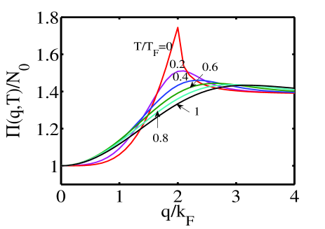
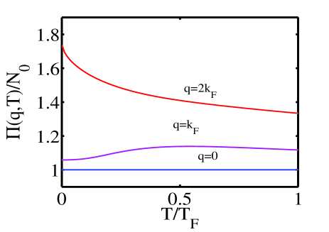
Figure 1: Temperature-dependent BLG polarizability (a) as a function of wave vector for different temperatures and (b) as a function of temperature for different wave vectors. Here $N_{0}=mg/2\pi$.

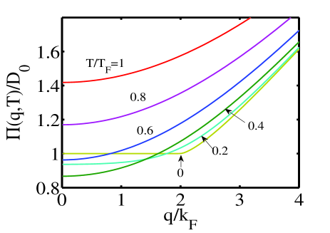
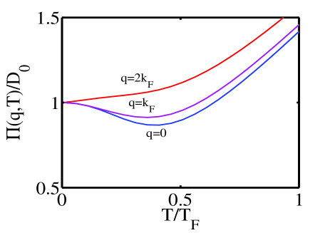
Figure 2: Temperature-dependent SLG polarizability (a) as a function of wave vector for different temperatures and (b) as a function of temperature for different wave vectors. Here $D_{0}=gk_{F}/(2\pi v_{F})$.

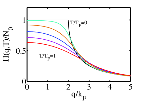
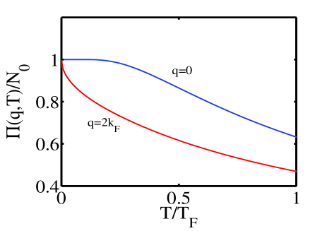
Figure 3: The 2DEG polarizability function (a) as a function of wave vector for several different temperatures $T/T_{F}=0,0.2,0.4,0.6,0.8,1.0$ (top to bottom). (b) as a function of temperature for different wave vectors. Here $N_{0}=mg/\pi$.

The BLG finite-temperature polarizability $\Pi(q,T)$ as a function of wave vector for different temperatures and as a function of temperature for different wave vectors are shown in Fig.1 (a) and (b), respectively. One novel phenomenon is that at $q=0$, the BLG polarizability equals to a constant value for all temperatures, $i.e.$, $\Pi(q=0,T)=N_{0}$. This is a qualitative difference between BLG and SLG (or 2DEG) polarizability function, while the latter $\Pi(q=0,T)$ as a function of temperature changes notably (as shown in Fig.2 for SLG and in Fig.3 for 2DEG). The reason is, at $q=0$, the intraband transition polarization $\Pi_{intra}(0,T)=N_{0}$ while the interband transition polarization $\Pi_{inter}(0,T)=0$, $i.e.$, the interband transition is forbidden at zero momentum transfer for all temperatures. The other remarkable phenomenon is the BLG polarizabilty approaches a constant value $N_{0}\log{4}$ in the large wave vector regime, arising from the fact that the interband transition dominates over the intraband contribution in the large wave vector limit. Therefore the dominative contribution to the whole polarizability has a crossover from intraband transition to interband transition for all temperatures. The weak temperature-dependent behavior of polarizations in the small and large wave vector regimes is a distinctive electronic property of BLG. Different from that of BLG, as shown in Fig.2(a), the polarizability of SLG increases monotonically for large $q$ stemming from the domination of exciting electrons from the valence band to the conduction band while the polarizability of 2DEG in large $q$ limit decreases as $1/{q^{2}}$ (as shown in Fig.3(a)).

In contrast to the SLG and the 2DEG, the polarizability of BLG as a function of wave vector shows a nonmonotonicity, $i.e.$, the polarizability at $T=0$ is monotone increasing with $q$ in the regime $[0,2k_{F}]$ and monotone decreasing in the regime larger than $2k_{F}$. In ordinary screened Coulomb scattering, the most dominant scattering happens at $q=2k_{F}$, which gives rise to the famous Friedel oscillations. Due to its sublattice symmetry, the $2k_{F}$ backward scattering of SLG is suppressed and therefore there is no singular behavior happen at $q=2k_{F}$. However, in BLG the $2k_{F}$ backscattering is restored and even enhanced because of its chirality, which leads to a sharp cusp and a discontinuous derivation of polarizability at $T=0$. We find that the temperature dependence of BLG polarizability at $q=2k_{F}$ is similar to that of 2DEG polarizability, both are much stronger than that of SLG polarizability. Due to the strong temperature dependence of the polarizability function at $q=2k_{F}$, as shown below, the BLG would have a anomalously strong temperature-dependent resistivity for $T\ll T_{F}$ which is similar to that of the regular 2D systems [17]. We also find the strong thermal suppression of the singular behavior of polarizability at $q=2k_{F}$, which is similar to that of the 2DEG.

Showing the difference between BLG and other 2D systems, we provide the polarizability functions of SLG and regular 2DEG in the regimes of $q=0$ and $q=2k_{F}$ in the low ($T\ll T_{F}$) and high ($T\gg T_{F}$) temperature limits. For $T\ll T_{F}$,

$$\Pi(q=0,T) \approx \left\{\begin{array}[]{ll}D_{0}[1-\frac{\pi^{2}}{6}(\frac{T}{T_{F}})^{2}]&(for\hskip 8.53581ptSLG)\\ \\ N_{0}[1-e^{-T_{F}/T}]&(for\hskip 8.53581pt2DEG)\end{array}\right.$$ (47)

$$\Pi(q=2k_{F},T) \approx \left\{\begin{array}[]{ll}D_{0}\left\{\frac{\mu(T)}{E_{F}}+\sqrt{\frac{\pi\mu}{2E_{F}}}\left[1-\frac{\sqrt{2}}{2}\right]\zeta\left(\frac{3}{2}\right)\left(\frac{T}{T_{F}}\right)^{3/2}\right\}&(for\hskip 8.53581ptSLG)\\ \\ N_{0}\left[1-\sqrt{\frac{\pi}{4}}\left(1-\sqrt{2}\right)\zeta\left(\frac{1}{2}\right)\left(\frac{T}{T_{F}}\right)^{1/2}\right]&(for\hskip 8.53581pt2DEG)\end{array}\right.$$ (51)

here $D_{0}=gE_{F}/2\pi v_{F}^{2}$ and $N_{0}=gm/2\pi$ are the density of states of SLG and regular 2DEG at Fermi level, respectively. Comparing to the corresponding screening formula for BLG,

$$\Pi(q=0,T) = N_{0},$$ (52)

$$\Pi(q=2k_{F},T) \approx N_{0}[C-\sqrt{\frac{\pi}{4}}(1-\sqrt{2})\zeta(\frac{1}{2})(\frac{T}{T_{F}})^{1/2}].$$ (53)

We can find at $q=2k_{F}$ the zero-temperature value of polarizability (normalized to the density of states at Fermi level) of BLG is different from that of 2DEG, but their temperature-dependent parts are both the same, which represents the similarity of BLG and 2DEG.

For $T\gg T_{F}$,

$$\Pi(q,T) \approx \left\{\begin{array}[]{ll}D_{0}\frac{T}{T_{F}}[\ln{4}+\frac{q^{2}}{24k_{F}^{2}}(\frac{T_{F}}{T})^{2}]&(for\hskip 8.53581ptSLG)\\ \\ N_{0}\frac{T_{F}}{T}\left[1-\frac{q^{2}}{6k_{F}^{2}}\frac{T_{F}}{T}\right]&(for\hskip 8.53581pt2DEG)\end{array}\right.$$ (57)

The corresponding high-temperature screening formula for BLG is given by

$$\Pi(q,T)\approx N_{0}\left[1+\frac{q^{2}}{6k_{F}^{2}}\frac{T_{F}}{T}\right].$$ (58)

In high temperature limit, the polarizability of BLG approaches a constant value ($i.e.~{}N_{0}$), which is very different from that of SLG, where the static polarizability increases linearly with $T$, and the regular 2DEG, where the polarizability falls as $1/T$. The BLG shows an intermediate behavior between the SLG and the regular 2DEG.

4 Conductivity Results

4.1 Analytic Asymptotic Results

In this section, we study analytically the static conductivity of the BLG in low and high temperatures limit. Firstly let us consider the temperature dependence of conductivity in the low temperature limit ($T\ll T_{F}$). Using Eq.(17), the scattering time $\tau(\varepsilon_{F},T)$ at the Fermi level $\varepsilon_{F}$ in the Born approximation is given as

$$\frac{1}{\tau(\varepsilon_{F},T)}=\frac{n_{i}}{2\pi\varepsilon_{F}}\int_{0}^{2k_{F}}dq\frac{q^{2}[1-2(q/2k_{F})^{2}]^{2}}{\sqrt{4k_{F}^{2}-q^{2}}}\frac{v_{i}(q)^{2}}{\epsilon(q,T)^{2}}.$$ (59)

In the low temperature limit, with Eq.(34) and (35), we find the difference between the finite temperature polarizability $\Pi(q,T)$ and the zero temperature polarizability $\Pi(q,T=0)$ is just a second order $(\sim O(T^{2}))$ small quantity. Therefore, the scattering time can be written as

$$\frac{1}{\tau(\varepsilon_{F},T)}\approx\frac{1}{\tau(\varepsilon_{F},T=0)}+O(T^{2}),$$ (60)

where

$$\frac{1}{\tau(\varepsilon_{F},T=0)}=\frac{n_{i}}{2\pi\varepsilon_{F}}\int_{0}^{2k_{F}}dq\frac{q^{2}[1-2(q/2k_{F})^{2}]^{2}}{\sqrt{4k_{F}^{2}-q^{2}}}\frac{v_{i}(q)^{2}}{\epsilon(q,T=0)^{2}}.$$ (61)

It is easily seen that the $q\approx 2k_{F}$ singularity dominate the evaluation of the integral in Eq.(61), thus we have

$$\frac{1}{\tau(\varepsilon_{F},T=0)} \approx \frac{n_{i}}{2\pi\varepsilon_{F}}\left(\frac{2\pi e^{2}}{\kappa}\right)^{2}\frac{1}{[1+q_{TF}g_{0}(2k_{F})/2k_{F}]^{2}}\int_{0}^{1}dx\frac{x^{2}[1-2x^{2}]^{2}}{\sqrt{1-x^{2}}}$$ (62)

$$= \frac{\pi}{g}\varepsilon_{F}\frac{n_{i}}{n}\frac{1}{[C+2k_{F}/q_{TF}]^{2}},$$

where $n$ is the electron density, $q_{TF}=mge^{2}/\kappa$ is the 2D Thomas-Fermi screening wave vector, $C=g_{0}(2k_{F})=\sqrt{5}-\log[(1+\sqrt{5})/2]$.

Considering the scattering time $\tau(\varepsilon,T=0)$ with energy $\varepsilon=k^{2}/2m$, we have

$$\frac{1}{\tau(\varepsilon,T=0)}=\frac{n_{i}}{2\pi\varepsilon}\int_{0}^{2k}dq\frac{q^{2}[1-2(q/2k)^{2}]^{2}}{\sqrt{4k^{2}-q^{2}}}\frac{v_{i}(q)^{2}}{\epsilon(q,T=0)^{2}},$$ (63)

where

$$\epsilon_{1}(q,T=0)=1+v_{c}(q)N_{0}g_{0}(q).$$ (64)

Then we express $\epsilon(q,T=0)$ as

$$\epsilon(q,T=0)=\epsilon_{1}(q,T=0)[1-\frac{v_{c}(q)N_{0}f_{0}(q)}{\epsilon_{1}(q,T=0)}\theta(q-2k_{F})].$$ (65)

With Eq.(65), we can express $1/\tau(\varepsilon,T=0)$ as

$$\frac{1}{\tau(\varepsilon,T=0)}\approx\frac{1}{\tau_{0}(\varepsilon,T=0)}+\frac{1}{\tau_{1}(\varepsilon,T=0)},$$ (66)

where

$$\frac{1}{\tau_{0}(\varepsilon,T=0)}=\frac{n_{i}}{2\pi\varepsilon}\int_{0}^{2k}dq\frac{q^{2}[1-2(q/2k)^{2}]^{2}}{\sqrt{4k^{2}-q^{2}}}\frac{v_{i}(q)^{2}}{\epsilon_{1}(q,T=0)^{2}},$$ (67)

and

$$\frac{1}{\tau_{1}(\varepsilon,T=0)}=\frac{n_{i}}{\pi\varepsilon}\int_{2k_{F}}^{2k}dq\frac{q^{2}[1-2(q/2k)^{2}]^{2}}{\sqrt{4k^{2}-q^{2}}}\frac{v_{i}(q)^{2}}{\epsilon_{1}(q,T=0)^{2}}\frac{v_{c}(q)N_{0}f_{0}(q)}{\epsilon_{1}(q,T=0)}\theta(\varepsilon-\varepsilon_{F}).$$ (68)

For $\mid(\varepsilon-\varepsilon_{F})/\varepsilon_{F}\mid\ll 1$, we can write

$$\frac{1}{\tau_{0}(\varepsilon,T=0)}\approx\frac{1}{\tau(\varepsilon_{F},T=0)[1+A(\varepsilon-\varepsilon_{F})/\varepsilon_{F}]},$$ (69)

with $A=-\varepsilon_{F}\tau(\varepsilon_{F},T=0)\partial[1/\tau(\varepsilon_{F},T=0)]/\partial\varepsilon_{F}$. From Eq.(68) we use the same trick as that of Eq.(62) and obtain

$$\frac{1}{\tau_{1}(\varepsilon,T=0)}=\frac{n_{i}}{\pi\varepsilon}(\frac{v_{i}(2k_{F})}{\epsilon_{1}(2k_{F},T=0)})^{2}\frac{v_{c}(2k_{F})N_{0}}{\epsilon_{1}(2k_{F},T=0)}I_{1}\theta(\varepsilon-\varepsilon_{F}),$$ (70)

where

$$I_{1}=\int_{2k_{F}}^{2k}dq\frac{q^{2}[1-2(q/2k)^{2}]^{2}}{\sqrt{4k^{2}-q^{2}}}[\frac{2k_{F}^{2}+q^{2}}{2k_{F}^{2}q}\sqrt{q^{2}-4k_{F}^{2}}+\log{\frac{q-\sqrt{q^{2}-4k_{F}^{2}}}{q+\sqrt{q^{2}-4k_{F}^{2}}}}],$$ (71)

and for $\mid(\varepsilon-\varepsilon_{F})/\varepsilon_{F}\mid\ll 1$, we have

$$I_{1}=\pi k_{F}^{2}\frac{\varepsilon-\varepsilon_{F}}{\varepsilon_{F}}+O((\frac{\varepsilon-\varepsilon_{F}}{\varepsilon_{F}})^{2}).$$ (72)

With Eq.(66)-(72), the energy dependent conductivity at zero temperature is given as

$$\sigma(\varepsilon,T=0) = \frac{e^{2}v_{F}^{2}}{2}N_{0}\tau(\varepsilon,T=0)$$ (73)

$$\approx \frac{e^{2}v_{F}^{2}}{2}N_{0}\tau(\varepsilon_{F},T=0)\left[1+A\frac{\varepsilon-\varepsilon_{F}}{\varepsilon_{F}}-\frac{\tau_{0}(\varepsilon,T=0)}{\tau_{1}(\varepsilon,T=0)}\right]$$

where

$$\frac{\tau_{0}(\varepsilon,T=0)}{\tau_{1}(\varepsilon,T=0)}=\frac{4q_{TF}}{2k_{F}+Cq_{TF}}\frac{\varepsilon-\varepsilon_{F}}{\varepsilon_{F}}\theta(\varepsilon-\varepsilon_{F}).$$ (74)

Using the Kubo-Greenwood formula [18]

$$\sigma(\varepsilon_{F},T)=\frac{1}{4k_{B}T}\int_{0}^{\infty}d\varepsilon\frac{\sigma(\varepsilon,T=0)}{\cosh^{2}[(\varepsilon-\varepsilon_{F})/2k_{B}T]},$$ (75)

and substituting Eq.(73) and (74) into Eq.(75) with a consideration of Eq.(62), we obtain the analytic asymptotic behavior of BLG conductivity at low temperature as following

$$\sigma(T\ll T_{F})=\sigma_{0}^{2D}\left(1-\frac{4\log{2}}{C+1/q_{0}}\frac{T}{T_{F}}\right),$$ (76)

where $q_{0}=q_{TF}/2k_{F}$ and $\sigma_{0}^{2D}=e^{2}v_{F}^{2}N_{0}\tau(\varepsilon_{F},T=0)/2$.

For high temperature limit, substituting Eq.(22) into Eq. (15), we have

$$\sigma(T\gg T_{F})=\sigma_{1}^{2D}\frac{\pi^{2}}{6}\left(\frac{T}{T_{F}}\right)^{2}\left(1+C_{h}q_{0}\sqrt{\frac{T_{F}}{T}}\right),$$ (77)

with $C_{h}=3.57$ and $\sigma_{1}^{2D}=(e^{2}/h)(n/n_{i})(g^{2}/\pi q_{0}^{2})$.

We show our numerical results of the conductivity and analytic asymptotic result of Eq.(76) in Fig.4, and find that they are excellently agreement with the numerical results in the low temperature limit.

It is significative to compare the conductivity temperature behaviors of SLG, BLG and 2DEG. For SLG, the asymptotic low and high temperature behaviors of conductivity are given by [15]

$$\sigma(T\ll T_{F})=\sigma_{0}\left[1-C_{0}\frac{\pi^{2}}{3}\left(\frac{T}{T_{F}}\right)^{2}\right],$$ (78)

$$\sigma(T\gg T_{F})=\sigma_{0}\frac{16I_{0}}{\pi}\left[4\log({2})r_{s}\right]^{2}\left(\frac{T}{T_{F}}\right)^{2},$$ (79)

here $\sigma_{0}\equiv\sigma(T=0)$, $C_{0}\sim o(1)$ and $I_{0}=0.034$. For 2DEG as found in Si MOSFETs and GaAs heterostructures, the asymptotic low and high temperature behaviors of conductivity are written as [19]

$$\sigma(T\ll T_{F})\approx\sigma_{0}^{2D}\left[1-C_{1}\left(\frac{T}{T_{F}}\right)\right],$$ (80)

$$\sigma(T\gg T_{F})\approx\sigma_{1}^{2D}\left[\frac{T}{T_{F}}+\frac{3\sqrt{\pi}q_{0}}{4}\sqrt{\frac{T_{F}}{T}}\right].$$ (81)

here $\sigma_{0}^{2D}\equiv\sigma(T=0)$, and $C_{1}=2q_{0}/(1+q_{0})$, $\sigma_{1}^{2D}=(e^{2}/h)(n/n_{i})(g^{2}/\pi q_{0}^{2})$ where $q_{0}=q_{TF}/2k_{F}$.

Now let us compare the BLG temperature dependence with the SLG and the regular parabolic 2D systems. First, for $T\ll T_{F}$, all the three systems show metallic temperature-dependent behaviors, but their strengthes of temperature dependence are different. BLG and the parabolic 2D system both have strong linear temperature dependence while SLG has a weak quadratic temperature dependence. Second, for high temperature limit $T\gg T_{F}$, BLG represents a quadratic temperature-dependent behavior which is similar to SLG, compared with the linear temperature dependence in the parabolic 2D system. Therefore, in the low temperature regime, the temperature-dependent transport of BLG is qualitatively similar to that of the parabolic 2D system, but as the temperature increasing, BLG is getting more and more similarity with SLG. The transport property of BLG as the intermediate between SLG and the regular 2DEG has been shown here.

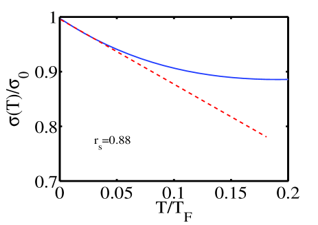
Figure 4: Numerical results of temperature-dependent conductivity of BLG in the low temperature region and its asymptotic form given by Eq.(76). The asymptotic form fits well in the regime $T\sim T_{F}[0,0.04]$. Here $\sigma_{0}=e^{2}v_{F}^{2}N_{0}\tau(\varepsilon_{F},T=0)/2$.

4.2 Numerical Results

We show the numerical results of resistivities obtained from Eq.(15) as a function of temperature for different $r_{s}$ values in Fig.5. $r_{s}=0.88$ corresponds to substrate-mounted ($\kappa=4$) bilayer graphene and $r_{s}=3.51$ corresponds to suspended ($\kappa=1$) bilayer graphene. It is found that the numerical results of BLG resistivity show metallic behavior at low temperature and insulating behavior at high temperature, which is the same as SLG and the regular 2D systems. Unlike graphene the scaled temperature-dependent resistivity of BLG has a relatively strong dependence on $r_{s}$ which is similar to that of the regular 2D systems. Because of the strong $q=2k_{F}$ backward scattering occurring in these two systems, this similarity also represents in the low temperature regime, where both of them have strong linear $T$ metallic behaviors with slopes $4\log{2}/(C+1/q_{0})$ for BLG and $2/(1+1/q_{0})$ for 2DEG. With temperature increasing, the BLG temperature-dependent behavior of resistivity is changing from 2DEG-like to SLG-like (falling off rapidly as $\sim 1/T^{2}$).

For comparison we show the calculated temperature-dependent resistivity of SLG and ordinary 2D systems for different interaction parameters $r_{s}$ in Fig.6 (for SLG) and Fig.7 (for ordinary 2D system). These two figures come from Ref.[15]. It is intuitively seen that at low temperature the linear $T$ behavior of BLG is similar to that of ordinary 2D system. However, the linear $T$ regime is rather weak and narrow for BLG, which is about $T\sim T_{F}[0,0.04]$ for $r_{s}=0.88$, while the linear $T$ regime for ordinary 2D system is relatively strong and broad, which extends from zero temperature to about $0.5T_{F}$ for $r_{s}=2.6$. Therefore in BLG, this screening-induced linear $T$ behavior is easily suppressed by other effects.

Since the Wigner-Seitz radius $r_{s}$, representing the strength of electron-electron interaction, is reasonably small ($r_{s}\approx 0.88$ for carrier density $n\sim 10^{12}cm^{-2}$), as shown in Fig.5 the temperature dependence arising from screening is rather weak in the BLG(the resistivity of BLG for $r_{s}=3.51$ decreases just about $14$ percents from $T/T_{F}=0$ to $T/T_{F}=1$ while the increase of resistivity of 2DEG for $r_{s}=3.7$ exceeds $100$ percents from $T/T_{F}=0$ to $T/T_{F}=1$). The dimensionless temperature $T/T_{F}$ is also rather small because of the relatively high Fermi temperature in BLG ($T_{F}\sim 400K$ for $n\sim 10^{12}cm^{-2}$). Therefore, as investigated experimentally in Ref. [11] and argued in Ref. [16], the strong collisional broadening effects due to the very small mobilities of current BLG samples would suppress the weak screening-induced temperature dependence that we calculated at low temperature ($i.e.,T\ll T_{F}$) and there would be no much temperature dependence in the low temperature resistivity. We hope our results to be tested in future experiments.

We show the temperature-dependent conductivity of BLG for different temperatures calculated as a function of carrier density in Fig.8. It shows that the conductivity increases in the low density regime and decrease in the high density regime as the temperature increases, representing a non-monotonic behavior of the conductivity.

In this article, we have assumed an ideal 2D BLG electron gas and ignored the distance $d$ between bilayer graphene and the charged impurity located at the substrate, which would make the form of potential of the charged impurity become $2\pi e^{2}e^{-qd}/\kappa(q+q_{TF})$. We also have assumed a homogeneous carrier density model, and therefore our theory is quantitatively correct only in the relatively high-density regime where the spatially inhomogeneous effects arising from charged impurity-induced electron-hole puddles are weak. For just comparing theoretically the screening-induced temperature-dependent behaviors of different 2D systems ($i.e.$, BLG, SLG and 2DEG), we do not take the level broadening effects due to impurity-scattering into account.

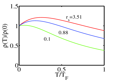
Figure 5: Numerical results of resistivities obtained from Eq.(15) as a function of temperature $T/T_{F}$ for different $r_{s}=3.51,0.88,0.1$ (from top to bottom). $r_{s}=0.88(3.51)$ corresponds to substrate-mounted (suspended) BLG. As $r_{s}$ increases the metallic behavior becomes stronger.

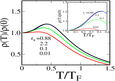
Figure 6: Numerical results of resistivities as a function of temperature $T/T_{F}$ for different $r_{s}=0.88$, 2.2, 0.1, 0.01 (from top to bottom). $r_{s}=0.88$ (2.2) corresponds to graphene on the SiO₂ substrate (in vacuum). Inset shows the magnified view in the low temperature limit $T<0.5T_{F}$. This figure comes from Ref. [15].

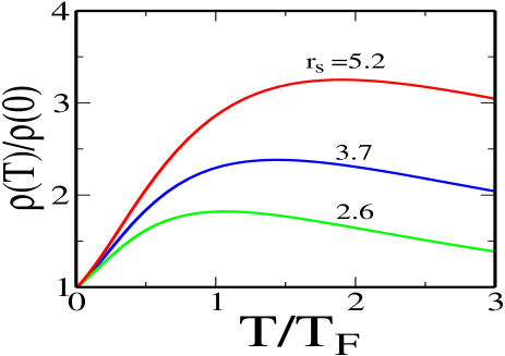
Figure 7: $\rho(T)/\rho(0)$ of an ordinary 2D system for different $r_{s}$ values as a function of temperature. As $r_{s}$ increases the metallic behavior becomes stronger. Compering to Fig. 5, the metallic behavior of the ordinary 2D system is much stronger than that of the BLG. This figure comes from Ref. [15].

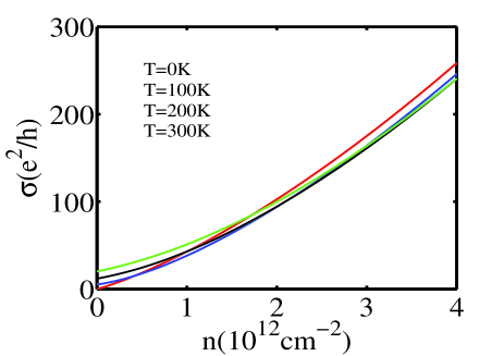
Figure 8: Calculated conductivity for different temperatures $T=0,100,200,300K$ (bottom to top in low density regime) as a function of density. Here we use $r_{s}=0.88$ and an impurity density $n_{i}=5\times 10^{11}cm^{-2}$.

5 Conclusions

In this article, we calculate the static wave vector polarizability of doped bilayer graphene at finite temperature under the RPA. We find that for all temperatures, the BLG static screening is equal to its density of states $N_{0}$ at zero momentum transfer and enhanced by a factor of $\log{4}$ at large momentum transfer. Due to the enhanced $q=2k_{F}$ backward scattering arising from the chirality of the BLG, a strong cusp of polarizability occurs at $q=2k_{F}$ for zero temperature but strongly thermal suppressed as temperature increases. Using a microscopic transport theory for BLG conductivity at finite temperature, we also obtain the asymptotic low and high temperature behaviors of conductivity for BLG, and find it has a linear temperature metallic behavior similar to the regular 2D system at low temperature and a quadratic temperature insulating behavior similar to the SLG. This crossover from 2DEG-like behavior to SLG-like behavior as temperature increases represents the unique transport properties of BLG as intermediate between the SLG and the regular 2DEG.

References

• [1] K. S. Novoselov, A. K. Geim, S. V. Morozov, D. Jiang, Y. Zhang, S. V. Dubonos, I. V. Grigorieva, and A. A. Firsov, Science 306, 666 (2004).
• [2] M. I. Katsnelson, Eur. Phys. J. B 51, 157 (2006); E. Fradkin, Phys. Rev. B 33, 3257 (1986); A. W. W. Ludwig, M. P. A. Fisher, R. Shankar, and G. Grinstein, Phys. Rev. B 50, 7526 (1994); N. Shon and T. Ando, J. Phys. Soc. Jpn. 67, 2421 (1998); J. TworzydΕ‚o, B. Trauzettel, M. Titov, A. Rycerz, and C. W. J. Beenakker, Phys. Rev. Lett. 96,246802 (2006).
• [3] E. H. Hwang, S. Adam, and S. Das Sarma, Phys. Rev. Lett. 98, 186806 (2007).
• [4] S. Adam, E. H. Hwang, V. M. Galitski, and S. Das Sarma, Proc. Natl. Acad. Sci. USA 104,18392 (2007).
• [5] E. Rossi, S. Adam, and S. Das Sarma, Phys. Rev. B 79, 245423 (2008).
• [6] E. H. Hwang and S. Das Sarma, Phys. Rev. B 75, 205418 (2007).
• [7] T. Ando, J. Phys. Soc. Jpn. 75, 074716 (2006).
• [8] B. Wunsch, T. Stauber, F. Sols, and F. Guinea, New J. Phys. 8, 318 (2006).
• [9] Y. Barlas et al., Phys. Rev. Lett. 98, 236601 (2007).
• [10] E. McCann and V. I. Fal’ko, Phys. Rev. Lett. 96, 086805 (2006); J. Nilsson, A. H. Castro Neto, N. M. R. Peres, and F. Guinea, Phys. Rev. B 73, 214418 (2006); B. Partoens and F. M. Peeters, Phys. Rev. B 74, 075404 (2006); M. Koshino and T. Ando, Phys. Rev. B 73, 245403 (2006); I. Snyman and C. W. J. Beenakker, Phys. Rev. B 75, 045322 (2007).
• [11] S. Morozov, K. Novoselov, M. Katsnelson, F. Schedin, D. Elias, J. Jaszczak, and A. Geim, Phys. Rev. Lett. 100, 016602 (2008);
• [12] K. Novoselov et al., Nature Phys. 2, 177 (2006); J. Oostinga et al., Nature Mater. 7, 151 (2008).
• [13] Y. Zhang, T-T. Tang, C. Girit, Z. Hao, M. C. Martin, A. Zettl, M. F. Crommie, Y. R. Shen and F. Wang, Nature 459, 820 (2009).
• [14] E. H. Hwang and S. Das Sarma Phys. Rev. Lett. 101, 156802 (2008).
• [15] E. H. Hwang and S. Das Sarma Phys. Rev. B 79, 165404 (2008).
• [16] S. Adam and S. Das Sarma Phys. Rev. B 77, 115436 (2008).
• [17] S. Das Sarma and E. H. Hwang, Phys. Rev. Lett. 83, 164 (1999).
• [18] J. M. Ziman, E​l​e​c​t​r​o​n​s​a​n​d​P​h​o​n​o​n​sπΈπ‘™π‘’π‘π‘‘π‘Ÿπ‘œπ‘›π‘ π‘Žπ‘›π‘‘π‘ƒβ„Žπ‘œπ‘›π‘œπ‘›π‘ ElectronsandPhonons (Oxford University Press, London, 1960).
• [19] S. Das Sarma and E. H. Hwang, Phys. Rev. B 68, 195315 (2003); S. Das Sarma and E. H. Hwang, Phys. Rev. B 69, 195305 (2004).