Non-Markovian dynamics without using quantum trajectory

Abstract

Open quantum system interacting with structured environment is important and manifests non-Markovian behavior, which was conventionally studied using quantum trajectory stochastic method. In this paper, by dividing the effects of the environment into two parts, we propose a deterministic method without using quantum trajectory. This method is more efficient and accurate than stochastic method in most Markovian and non-Markovian cases. We also extend this method to the generalized Lindblad master equation.

When an open quantum system interacts with environment, it experiences decoherence and dissipation which lead to loss of information. Such open quantum system is depicted by a reduced density matrix which shows non-unitary evolution. On the other hand, the environment is classified as Markovian with no memory effect, and non-Markovian with memory effect. In Markovian case, since there is no memory effect, the quantum trajectory based Monte Carlo wave function (MCWF) method QJ1 ; QJ3 ; MCM and quantum state diffusion (QSD) method QSDM1 ; QSDM2 are applied. However, in non-Markovian case, due to memory effect, the information lost by the system during the interaction with the environment will come back to the system in a later time and so shows much more complicated behaviors than Markovian case.

Non-Markovian systems are important for their applications to many fields of physics, such as quantum information processing quantum information ; LiZhou , quantum optics OQS , solid state physics solid state physics , and chemical physics chemical physics . Recently, non-Markovian behaviors have also been studied in biomolecules where the molecules are embedded in a solvent and/or in a protein environment biomolecules . Since there is no true pure state quantum trajectory due to the memory effect no single trajectory , the quantum trajectory based Markovian methods do not work. Thus, doubled Hilbert space (DHS) method DHS , triple Hilbert space (THS) method THS , non-Markovian QSD method QSD1 ; QSD2 , and non-Markovian quantum jump (NMQJ) method NMQJ1 ; NMQJ2 are proposed to solve the non-Markovian dynamics of the system where the memory effect is taken into account. However, in order to obtain high accuracy, all these methods, which are based on stochastic simulations, need to fulfill a large number of realizations and is very time-consuming. So, new methods which are more efficient and accurate are highly desired.

In this paper, a deterministic method without using quantum trajectory is proposed to solve the non-Markovian dynamics. The influence of the environment on the system is divided into two parts, i.e., the non-unitary evolution of the states and the probability flow between these states. Moreover, we also extend this approach to the generalized Lindblad master equation which can deal with some strong coupling cases GLE . The algorithm and numerical efficiency are given, which show that our method is more efficient and accurate than those based on stochastic simulation in most Markovian and non-Markovian cases.

The dynamics of the non-Markovian system is governed by the following master equation OQS

$$\begin{split}\dot{\rho}(t)=&\displaystyle\frac{1}{{i\hbar}}[H_{s},\rho(t)]+\sum\limits_{j}{\gamma_{j}(t)C_{j}(t)\rho(t)C_{j}^{\dagger}(t)}\\ &-\displaystyle\frac{1}{2}\sum\limits_{j}{\gamma_{j}(t)\{\rho(t),C_{j}^{\dagger}(t)C_{j}(t)\}},\\ \end{split}$$ (1)

where $H_{s}$ is the system Hamiltonian including the Lamb shift, $C_{j}(t)$ are the jump operators which induce changes [e.g., jump from state $\psi_{\alpha}(t)$ to $\psi_{\alpha^{\prime}}(t)$ i.e., $|\psi_{\alpha^{\prime}}(t)\rangle=C_{j}(t)|\psi_{\alpha}(t)\rangle/\left|\left|C_{j}(t)|\psi_{\alpha}(t)\rangle\right|\right|$ ] in the system, and $\gamma_{j}(t)$ are the decay rates which may take negative values for some time intervals. The reduced density matrix can be written as NMQJ1

$$\rho(t)=\sum_{\alpha=1}^{N_{eff}}p_{\alpha}(t)|\psi_{\alpha}(t)\rangle\langle\psi_{\alpha}(t)|,$$ (2)

where $p_{\alpha}(t)$ is the probability of the system being in the state $|\psi_{\alpha}(t)\rangle$ at time $t$. Further, it should be pointed out that the effective number of the states $N_{eff}$ is determined by $C_{j}(t)$’s NMQJ2 , $\sum_{\alpha=1}^{N_{eff}}p_{\alpha}(t)=1$ and that the state $|\psi_{\alpha}(t)\rangle$ is normalized.

To solve the dynamics of the system, one should know the time evolution of $|\psi_{\alpha}(t)\rangle$ and its probability $p_{\alpha}(t)$. In our method, the time evolution of the state $|\psi_{\alpha}(t)\rangle$ is the same as that in NMQJ NMQJ1 . In NMQJ, the probability $p_{\alpha}(t)$ is calculated in a stochastic way by using quantum trajectory to $N$ ensemble members. In our method, however, the evolution of probability $p_{\alpha}(t)$ is given in a deterministic way:

$$\dot{p}_{\alpha}(t)=-\sum_{j}\Gamma_{\alpha}^{j}(t)p_{\alpha}(t)+{\sum_{(\alpha^{\prime},j)}}^{\prime}\Gamma_{\alpha^{\prime}}^{j}(t)p_{\alpha^{\prime}}(t),$$ (3)

where $\Gamma_{\alpha}^{j}(t)={\gamma_{j}(t)}{\left\|{C_{j}(t)\left|{\psi_{\alpha}(t)}\right\rangle}\right\|}^{2}$ and ${\sum\limits_{(\alpha^{\prime},j)}}^{\prime}$represents the summation over all the pairs $(\alpha^{\prime},j)$ satisfying $\left|{\psi_{\alpha}(t)}\right\rangle={{C_{j}(t)\left|{\psi_{\alpha^{\prime}}(t)}\right\rangle}\mathord{\left/{\vphantom{{C_{j}(t)\left|{\psi_{\alpha^{\prime}}(t)}\right\rangle}{\left\|{C_{j}(t)\left|{\psi_{\alpha^{\prime}}(t)}\right\rangle}\right\|}}}\right.\kern-1.2pt}{\left\|{C_{j}(t)\left|{\psi_{\alpha^{\prime}}(t)}\right\rangle}\right\|}}$. One finds that the probability of the state, $p_{\alpha}(t)$, changes via the mechanism of jumps for “out” ($\alpha\to\alpha^{\prime}$) and “in” ($\alpha^{\prime}\to\alpha$), respectively.

The numerical simulation corresponding to Eq. (3) is straightforward:

$$p_{\alpha}(t+\delta t)=p_{\alpha}(t)-\delta t\sum_{j}\Gamma_{\alpha}^{j}(t)p_{\alpha}(t)+\delta t{\sum_{(\alpha^{\prime},j)}}^{\prime}\Gamma_{\alpha^{\prime}}^{j}(t)p_{\alpha^{\prime}}(t).$$ (4)

Note that there is no stochastic noise and no need to consider the sign of the decay rate during the simulation. Additionally, the $p_{\alpha}(t)$’s in our method do represent the probability of the system actually being in the corresponding pure state ensemble.

Consider a particular transition: $|\psi_{\alpha^{\prime}}(t)\rangle=C_{j}(t)|\psi_{\alpha}(t)\rangle/\left|\left|C_{j}(t)|\psi_{\alpha}(t)\rangle\right|\right|$, then the corresponding probability change takes the form:

$$\begin{split}p_{\alpha}(t+\delta t)&=p_{\alpha}(t)-\delta tp_{\alpha}(t)\Gamma_{\alpha}^{j}(t),\\ p_{\alpha^{\prime}}(t+\delta t)&=p_{\alpha^{\prime}}(t)+\delta tp_{\alpha}(t)\Gamma_{\alpha}^{j}(t).\\ \end{split}$$ (5)

When the decay rate $\gamma_{j}(t)$ is positive or negative, the probability flow is from $\left|{\psi_{\alpha}(t)}\right\rangle$ to $|\psi_{\alpha^{\prime}}(t)\rangle$ or reversed. This has been mentioned in Ref.NMQJ1 . However, it is more explicit in our method. From Eq. (5), it is clear that, in the negative decay region, the amount of probability flow only depends on the target state and the probability of the system being in the target state. This is similar to the situation in NMQJ NMQJ1 , where the jump probability in the negative decay region is proportional to the number of particles in the target state. These indicate that the trajectory of a particle in NMQJ can not be interpreted as true trajectory since the jump process depends on the status of other particles in the system. Because true pure state quantum trajectories do not exist in the non-Markovian dynamics no single trajectory , it is not necessary to calculate $p_{\alpha}(t)$ in a stochastic way.

Next, we extend our method to the recently proposed generalized Lindblad master equation which can solve the dynamics of some highly non-Markovian systemsGLE ,

$$\frac{d}{{dt}}{\rho_{i}}=-i[{H_{i}},{\rho_{i}}]+\sum\limits_{j\lambda}{\left({R_{\lambda}^{ij}{\rho_{j}}R{{{}_{\lambda}^{ij}}^{\dagger}}-\frac{1}{2}\{R{{{}_{\lambda}^{ji}}^{\dagger}}R_{\lambda}^{ji},{\rho_{i}}\}}\right)},$$ (6)

where $i,j=1,2,\cdots,n$, $H_{i}$ are any Hermitian operators, and $R_{\lambda}^{ij}$ are any system operators. It should be indicated that $\rho(t)=\sum\limits_{i=1}^{n}{{\rho_{i}}(t)}$.

The $i$th density matrix is decomposed as:

$${\rho_{i}}(t)=\sum\limits_{\alpha=1}^{N_{eff}^{i}}{p_{i}^{\alpha}(t)\left|{\psi_{i}^{\alpha}(t)}\right\rangle\left\langle{\psi_{i}^{\alpha}(t)}\right|},$$ (7)

where $N_{eff}^{i}$ is determined in the same way in Eq. (2) by taking all the jump operators ${R_{\nu}^{ij}}^{,}$s and all the states $\psi_{j}^{\alpha}(t)^{,}$s in each ${\rho_{j}}(t)$ into consideration.

The evolution of state $\left|{\psi_{i}^{\alpha}(t)}\right\rangle$ is governed by the nonlinear differential equationexample2

$$i\frac{d}{{dt}}\left|{\psi_{i}^{\alpha}(t)}\right\rangle=\hat{G}(\psi_{i}^{\alpha})(t)\left|{\psi_{i}^{\alpha}(t)}\right\rangle,$$ (8)

where $\hat{G}(\psi_{i}^{\alpha})(t)={H^{i}}-\frac{i}{2}\sum\limits_{j\nu}{R{{{}_{\nu}^{ji}}^{\dagger}}R_{\nu}^{ji}}+\frac{i}{2}\sum\limits_{j\nu}{{{\left\|{R_{\nu}^{ji}\left|{\psi_{i}^{\alpha}(t)}\right\rangle}\right\|}^{2}}}$. By combining Eqs. (6), (7), (8) and noting that ${\left|{\psi_{i}^{1}(t)}\right\rangle\left\langle{\psi_{i}^{1}(t)}\right|}$, ${\left|{\psi_{i}^{2}(t)}\right\rangle\left\langle{\psi_{i}^{2}(t)}\right|}$, $\cdots$, ${\left|{\psi_{i}^{N_{eff}^{i}}(t)}\right\rangle\left\langle{\psi_{i}^{N_{eff}^{i}}(t)}\right|}$ are linearly independent, the evolution of $p_{i}^{\alpha}(t)$ is given by

$$\dot{p}_{i}^{\alpha}(t)=-\sum\limits_{j\nu}{\Gamma_{\nu\alpha}^{ji}}p_{i}^{\alpha}(t)+{\sum\limits_{(j,\nu,\alpha^{\prime})}}^{\prime}{\Gamma_{\nu\alpha^{\prime}}^{ij}p_{j}^{\alpha^{\prime}}(t)},$$ (9)

where $\Gamma_{\nu\alpha}^{ij}={\left\|{R_{\nu}^{ij}\left|{\psi_{j}^{\alpha}(t)}\right\rangle}\right\|^{2}}$ and ${\sum\limits_{(j,\nu,\alpha^{\prime})}}^{\prime}$ represents the summation over all the pairs $(j,\nu,\alpha^{\prime})$ satisfying $\left|{\psi_{i}^{\alpha}(t)}\right\rangle={{R_{\nu}^{ij}\left|{\psi_{j}^{\alpha^{\prime}}(t)}\right\rangle}\mathord{\left/{\vphantom{{R_{\nu}^{ij}\left|{\psi_{j}^{\alpha^{\prime}}(t)}\right\rangle}{\left\|{R_{\nu}^{ij}\left|{\psi_{j}^{\alpha^{\prime}}(t)}\right\rangle}\right\|}}}\right.\kern-1.2pt}{\left\|{R_{\nu}^{ij}\left|{\psi_{j}^{\alpha^{\prime}}(t)}\right\rangle}\right\|}}$. It can be easily seen that by setting $n=1$ and taking the decay rates $\gamma(t)$ into the equation, Eq. (9) degenerates to Eq. (3).

Example $1$: Detuned Jaynes-Cummings model.–Consider a system with a two-level atom in a detuned damped cavity, which is governed by the time convolutionless master equation OQS

$$\begin{split}\dot{\rho}(t)=&-\displaystyle\frac{i}{2}S(t)\{\sigma_{+}\sigma_{-},\rho(t)\}\\ &+\gamma(t)\{\sigma_{-}\rho(t)\sigma_{+}-\displaystyle\frac{1}{2}\sigma_{+}\sigma_{-}\rho(t)-\displaystyle\frac{1}{2}\rho(t)\sigma_{+}\sigma_{-}\}.\\ \end{split}$$ (10)

The spectral density of the cavity is supposed to be of Lorentzian profile, i.e., $J(\omega)=\frac{\gamma_{0}\lambda^{2}}{2\pi[(\omega_{0}-\Delta-\omega)^{2}+\lambda^{2}]},$ where $\Delta=\omega_{0}-\omega_{c}$ is the detuning between the cavity mode and the atom. To second order approximation, the Lamb shift and the decay rate take the form OQS $S(t)=\frac{{\gamma_{0}\lambda\Delta}}{{\lambda^{2}+\Delta^{2}}}\{1-{\mathop{\rm e}\nolimits}^{-\lambda t}[\cos(\Delta t)+\frac{\lambda}{\Delta}\sin(\Delta t)]\},$ $\gamma(t)=\frac{{\gamma_{0}\lambda^{2}}}{{\lambda^{2}+\Delta^{2}}}\{1-{\mathop{\rm e}\nolimits}^{-\lambda t}[\cos(\Delta t)-\frac{\Delta}{\lambda}\sin(\Delta t)]\}.$ In this model, there is only one jump operator $C=\sigma_{-}=\left|g\right\rangle\left\langle e\right|$, which is a lowering operator. We assume that $\rho(0)=\left|{\psi_{1}(0)}\right\rangle\left\langle{\psi_{1}(0)}\right|$ and choose $\left|{\psi_{1}(0)}\right\rangle=(4\left|e\right\rangle+3\left|g\right\rangle)/5$. Acting the jump operator on the state $\left|{\psi_{1}(0)}\right\rangle$, we get $\left|{\psi_{2}(0)}\right\rangle=\left|g\right\rangle$. According to Eq. (4), at time $t+\delta t$, the probabilities become

$$\begin{array}[]{l}p_{1}(t+\delta t)=p_{1}(t)-\delta tp_{1}(t)\Gamma_{1}^{1}(t),\\ p_{2}(t+\delta t)=p_{2}(t)+\delta tp_{1}(t)\Gamma_{1}^{1}(t),\\ \end{array}$$ (11)

where $\Gamma_{1}^{1}(t)=\gamma(t)\left|{\left\langle{e}\mathrel{\left|{\vphantom{e{\psi_{1}(t)}}}\right.\kern-1.2pt}{{\psi_{1}(t)}}\right\rangle}\right|^{2}.$

In this example, $\rho_{ee}(t)$ is proportional to the energy of the system and $p_{2}(t)$ represents the probability for one photon being in the environment. Although $p_{1}(t)$ and $p_{2}(t)$ can be solved analytically, in order to illustrate our method, we use Eq. (11) to do the simulation. The parameters are chosen as $\Delta=12\lambda,\gamma_{0}\lambda=4,\lambda\delta t=0.005$.

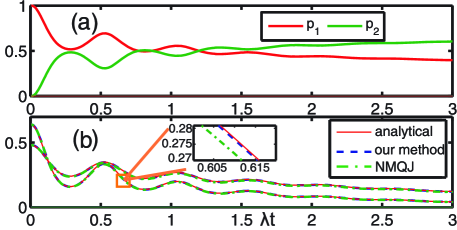
Figure 1: (color online) Dynamics of detuned Jaynes-Cummings model. The initial state is $\left|{\psi_{1}(0)}\right\rangle=(4\left|e\right\rangle+3\left|g\right\rangle)/5$ and the parameters are $\Delta=12\lambda,\gamma\lambda=4,\lambda\delta t=0.005$. (a) The probabilities for the system in states $\left|{\psi_{1}(t)}\right\rangle$ and $\left|{\psi_{2}(t)}\right\rangle$. (b) The population of the excited state $\rho_{ee}$ (initially higher line) and the absolute value of the coherence $\rho_{eg}$ (initially lower line) with three methods: analytic (red solid curve), our method (blue long-dashed curve) and NMQJ (with $N=10^{4}$ particles in the system, green dash-dot curve).

Figure 1 (a) shows explicitly the reversal of the probability flow. We can see from Fig. 1 (a) and (b) that when the probability flow gets reversed, the energy and coherence of the atom increase. These show explicitly the memory effect that the reduced system restores the information lost earlier. In Fig. 1 (b), the result of NMQJ (with $N=10^{4}$ particles in the system) is also given, which shows that our method is more accurate.

Example 2: Application to generalized Lindblad master equation.– To illustrate our method for this kind of equation, we consider a two-state system coupled to an environment consisting of two energy bands, each with a finite number of evenly spaced levels. This may be viewed as a spin coupled to a single molecule or a single particle quantum dot example21 . By using time-convolutionless projection operator technique, to the second order, the generalized Lindblad master equation takes the form example2

$$\begin{array}[]{l}\displaystyle\frac{d}{{dt}}\rho_{1}=\int_{0}^{t}{dt_{1}h(t-t_{1})}[2\gamma_{1}\sigma^{+}\rho_{2}\sigma^{-}-\gamma_{2}\{\sigma^{+}\sigma^{-},\rho_{1}\}],\\ \displaystyle\frac{d}{{dt}}\rho_{2}=\int_{0}^{t}{dt_{1}h(t-t_{1})}[2\gamma_{2}\sigma^{-}\rho_{1}\sigma^{+}-\gamma_{1}\{\sigma^{-}\sigma^{+},\rho_{2}\}],\\ \end{array}$$ (12)

where $\gamma_{i}h(t-t_{1}),(i=1,2),$ is the environment correlation function with $h(t)=\frac{{\delta\varepsilon\sin^{2}(\delta\varepsilon t/2)}}{{2\pi(\delta\varepsilon t/2)^{2}}}$ where $\delta\varepsilon$ is the width of the upper and lower energy bands. The reduced density matrix for the system is given by $\rho=\rho_{1}+\rho_{2}.$

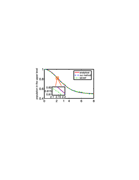
Figure 2: (color online) A two-state system coupled to an environment consisting of two energy bands. Comparison of our method (blue long-dashed curve) and Monte Carlo simulation (with $N=10^{4}$ trajectories, green dash-dot curve) to analytical result (red solid curve). The parameters are $\delta\epsilon=0.31,$ $\gamma_{1}=\gamma_{2}=1$ and time step $\delta t=0.01$.

We assume that $\rho_{1}(0)=\left|e\right\rangle\left\langle e\right|$ and $\rho_{2}(0)=0$. The parameters are chosen as $\delta\epsilon=0.31$ and $\gamma_{1}=\gamma_{2}=1$. In Fig. 2 we compare the results of our method, analytical solution and Monte Carlo simulation which is based on the unraveling of the master equation (with $N=10^{4}$ trajectories) example2 . Apparently, our method is more accurate than Monte Carlo simulation method.

According to Eqs. (4), we only need to calculate $N_{eff}$ states and change the probabilities deterministically. The time cost is almost determined by the calculation of $N_{eff}$ states. However, the evolution of $N_{eff}$ states is independent with each other, so we can calculate them parallelly. In addition, if the jump operators can be represented by sparse matrixes, we only need to calculate the evolution of the states appearing in the decomposition of $\rho(0)$ and use the jump operators to obtain other states. Moreover, since the sign of the decay rate makes no difference during the simulation, in non-Markovian case, our method is as efficient as it behaves in Markovian case.

Similar to our method, the NMQJ method NMQJ1 ; NMQJ2 needs to calculate $N_{eff}$ states. However, in addition to that, NMQJ has to consider the sign of the decay rates and generate $N$ random numbers ($N\gg N_{eff}$) to decide the jump process at each time step $\delta t$. Apparently, our method is more efficient than NMQJ in any case.

In Markovian case, the MCWF QJ1 and QSD QSDM1 method need to realize a large number of trajectories for every state appearing in the decomposition of $\rho(0)$. When the number of these trajectories is larger than $N_{eff}$, which is always the case, our method is more efficient than them. In non-Markovian case, the DHS method DHS , THS method THS and non-Markovian QSD method QSD1 ; QSD2 all introduce additional cost for computational efficiency compared to MCWF or QSD. However, in non-Markovian case, our method is as efficient as it behaves in Markovian case. Thus, when the number of these trajectories is larger than $N_{eff}$, our method is obviously more efficient than them, too.

As for the accuracy, since there is no statistical noise in our method and the error caused by finite time step $\delta t$ is the same, compared with all the methods based on stochastic simulation, our method is more accurate. Actually, our method is the limit case when the number of realizations in the stochastic based methods tends to infinite.

In conclusion, by dividing the influence of the environment on the system into two parts, i.e., the non-unitary evolution of these states and the probability flow between them, we propose a deterministic method to solve the non-Makovian dynamics. Compared with the method based on stochastic simulation, our method has advantages in efficiency and accuracy. Additionally, we extended this approach to the generalized Lindblad master equation , which is useful to solve the dynamics of some highly non-Markovian systems.

This work is supported by the Key Project of the National Natural Science Foundation of China (Grant No. 60837004).

References

(1) J. Dalibard, Y. Castin, and K. Mlmer, Phys. Rev. Lett. 68, 580 (1992);
(2) H. Carmichael, An Open System Approach to Quantum Optics, Lecture
Notes in Physics (Springer-Verlag, Berlin, 1993), Vol. m18.
(3) M. B. Plenio and P. L. Knight, Rev. Mod. Phys. 70, 101 (1998).
(4) N. Gisin and I. C. Percival, J. Phys. A 25, 5677 (1992); 26, 2233
(1993); 26, 2245 (1993).
(5) I. Percival, Quantum State Diffusion (Cambridge University Press,
Cambridge, England, 2002).
(6)M. A. Nielsen and I. L. Chuang, Quantum Computation and Quantum
Information (Cambridge University Press, Cambridge, England, 2000)
(7) Y. Li, J. Zhou, and H. Guo, Phys. Rev. A 79, 012309 (2009).
(8) H.-P. Breuer and F. Petruccione, The Theory of Open Quantum
Systems (Oxford University Press, Oxford, 2002).
(9)See, e.g., C. W. Lai, P.
Maletinsky, A. Badolato, and A. Imamoglu, Phys. Rev. Lett. 96,
167403 (2006), and references therein.
(10)J. Shao, J. Chem. Phys. 120, 5053 (2004); A. Pomyalov and D. J.
Tannor, J. Chem. Phys. 123, 204111 (2005) and references
therein.
(11)P. Rebentrost, R. Chakraborty, and A.
Aspuru-Guzik, J. Chem. Phys. 131, 184102 (2009).
(12)H. M. Wiseman and J. M. Gambetta, Phys. Rev. Lett. 101, 140401
(2008).
(13) H.-P. Breuer, B. Kappler, and F. Petruccione, Phys. Rev. A
59, 1633 (1999).
(14) H.-P. Breuer, Phys. Rev. A 70, 012106 (2004).
(15) W. T. Strunz, L. Disi, and N. Gisin, Phys. Rev. Lett.
82, 1801 (1999).
(16)J. T. Stockburger and H. Grabert, Phys. Rev. Lett. 88, 170407
(2002).
(17)J. Piilo, S. Maniscalco, K. Hrknen, and K.-A. Suominen, Phys. Rev. Lett. 100, 180402 (2008).
(18)J. Piilo, S. Maniscalco, K. Hrknen, and K.-A. Suominen, Phys. Rev. A 79, 062112 (2009).
(19)H.-P. Breuer, Phys. Rev. A 75, 022103 (2007).
(20)J. Gemmer and M. Michel, Europhys. Lett. 73, 1
(2006).
(21)M. Moodley and F. Petruccione, Phys. Rev. A 79, 042103 (2009).