Nonrelativistic Chern-Simons Vortices
on the Torus

Abstract

A classification of all periodic self-dual static vortex solutions of the Jackiw-Pi model is given. Physically acceptable solutions of the Liouville equation are related to a class of functions which we term $\Omega$-quasi-elliptic. This class includes, in particular, the elliptic functions and also contains a function previously investigated by Olesen. Some examples of solutions are studied numerically and we point out a peculiar phenomenon of lost vortex charge in the limit where the period lengths tend to infinity, that is, in the planar limit.

NIKHEF/2009-030

FERMILAB-PUB-09-590-T

1 Introduction

In this paper we study periodic, static vortex solutions of the Jackiw-Pi model [1, 2]. This is a $2+1$-dimensional nonrelativistic conformal field theory whose field content consists of a complex scalar field $\Psi$ with non-linear-Schrödinger type action minimally coupled to a $\mathrm{U}(1)$ Chern-Simons gauge field $A_{\mu}$. Let us begin by reviewing the elements of this model.

1.1 The Jackiw-Pi model

We take as our starting point the action [6]

$$\begin{array}[]{lll}S[\Psi,A_{\mu}]&=&\displaystyle{\int dx^{0}\int d^{2}x\,\Big{\{}-\frac{1}{2}\varepsilon_{ij}\left(A_{0}\partial_{i}A_{j}+A_{i}\partial_{j}A_{0}+A_{j}\partial_{0}A_{i}\right)}\\ &&\\ &&\displaystyle{\hskip 60.00009pt+\,i\Psi^{*}D_{0}\Psi-\frac{1}{2}\,(\mathbf{D}\Psi)^{*}\cdot(\mathbf{D}\Psi)-\frac{g^{2}}{2}|\Psi|^{4}\Big{\}}.}\end{array}$$ (1)

Here $\varepsilon_{12}=-\varepsilon_{21}=+1$, whilst $D_{\mu}=\partial_{\mu}-ieA_{\mu}$ is the gauge covariant derivative and bold type indicates its spatial 2-vector part. We use the generic notation $x^{0}$ for the time coordinate, and apply the summation convention for repeated indices. In the following we define

$$\begin{array}[]{l}\displaystyle{\rho=\Psi^{*}\Psi,\hskip 20.00003ptJ_{i}=-\frac{i}{2}\left(\Psi^{*}D_{i}\Psi-\Psi D_{i}\Psi^{*}\right),}\\ \\ B=\partial_{1}A_{2}-\partial_{2}A_{1},\hskip 20.00003ptE_{i}=\partial_{0}A_{i}-\partial_{i}A_{0}.\end{array}$$ (2)

The field equations derived from the action (1) then read

$$\begin{array}[]{l}B=e\rho,\hskip 20.00003ptE_{i}=e\varepsilon_{ij}J_{j},\\ \\ \displaystyle{iD_{0}\Psi=-\frac{1}{2}\,\mathbf{D}^{2}\Psi+g^{2}|\Psi|^{2}\Psi.}\end{array}$$ (3)

The chiral derivatives

$$D_{\pm}=\frac{1}{\sqrt{2}}\left(D_{1}\pm iD_{2}\right),$$ (4)

satisfy the identities

$$\frac{1}{2}\,\mathbf{D}^{2}=D_{-}D_{+}-\frac{e}{2}\,B=D_{+}D_{-}+\frac{e}{2}\,B.$$ (5)

Using equations (3), the Schrödinger equation for $\Psi$ can then be written as

$$iD_{0}\Psi=-D_{-}D_{+}\Psi+\left(g^{2}+\frac{e^{2}}{2}\right)|\Psi|^{2}\Psi=-D_{+}D_{-}\Psi+\left(g^{2}-\frac{e^{2}}{2}\right)|\Psi|^{2}\Psi.$$ (6)

By a similar argument, the hamiltonian takes the form

$$H=\int d^{2}x\left(\frac{1}{2}|\mathbf{D}\Psi|^{2}+\frac{g^{2}}{2}\,|\Psi|^{4}\right)=\int d^{2}x\left(|D_{\pm}\Psi|^{2}+\frac{1}{2}(g^{2}\pm e^{2})|\Psi|^{4}\right).$$ (7)

Hence there are two possibilities for constructing stationary zero-energy solutions:

$$\begin{array}[]{ll}(I)&D_{+}\Psi=0\hskip 10.00002pt\mbox{and}\hskip 10.00002ptg^{2}+e^{2}=0,\\ &\\ (II)&D_{-}\Psi=0\hskip 10.00002pt\mbox{and}\hskip 10.00002ptg^{2}-e^{2}=0.\end{array}$$ (8)

By stationary we mean that physical observables such as the particle density and current are time-independent. This is achieved by separating space and time variables as

$$\Psi=e^{i\omega}\sqrt{\rho},$$ (9)

with $\rho$ non-negative and time independent: $\partial_{0}\rho=0$. Any time dependence therefore resides in the gauge-dependent phase $\omega$.

Substitution of either of the Ansätze $(I)$ or $(II)$ for $\Psi$ and the coupling constants $(e,g)$ simplifies the Schrödinger equation (6) to

$$iD_{0}\Psi=(eA_{0}-\partial_{0}\omega)\Psi=\mp\frac{e^{2}}{2}\,|\Psi|^{2}\Psi\hskip 10.00002pt\Rightarrow\hskip 10.00002pteA_{0}=\partial_{0}\omega\mp\frac{e^{2}}{2}\,\rho.$$ (10)

In addition, the real and imaginary parts of either condition $D_{\pm}\Psi=0$ lead to the real equations

$$eA_{i}=\partial_{i}\omega\pm\varepsilon_{ij}\partial_{j}\ln\sqrt{\rho},$$ (11)

and as a result

$$eB=e\varepsilon_{ij}\partial_{i}A_{j}=\mp\Delta\ln\sqrt{\rho},\hskip 20.00003pt\Delta=\partial_{1}^{2}+\partial_{2}^{2}.$$ (12)

It follows directly that $\rho$ satisfies one of the Liouville equations

$$\begin{array}[]{ll}(I)&D_{+}\Psi=0\hskip 10.00002pt\Rightarrow\hskip 10.00002pt\Delta\ln\sqrt{\rho}+e^{2}\rho=0,\\ \\ (II)&D_{-}\Psi=0\hskip 10.00002pt\Rightarrow\hskip 10.00002pt\Delta\ln\sqrt{\rho}-e^{2}\rho=0.\end{array}$$ (13)

The solutions of these equations are respectively of the form [7]

$$\begin{array}[]{ll}(I)&\displaystyle{\rho_{f}=\frac{4}{e^{2}}\,\frac{|f^{\prime}|^{2}}{(1+|f|^{2})^{2}},}\\ \\ (II)&\displaystyle{\rho_{f}=\frac{4}{e^{2}}\,\frac{|f^{\prime}|^{2}}{(1-|f|^{2})^{2}},}\end{array}$$ (14)

where $f(z)$ is an analytic function of the complex coordinate

$$z=x+iy,$$ (15)

and for physical reasons we make the hypothesis that $f$ have at most isolated singularities (which then automatically are poles; see the discussion in Section 1.2).

Furthermore, boundedness of $\rho$ requires $|f|^{2}<1$ for case $(II)$. This immediately implies that there are no relevant non-trivial solutions in case $(II)$.

However, case $(I)$ leads to a rich spectrum of vortex-type solutions, depending on the boundary conditions. For instance, if we take two-dimensional space to be the plane $\mathbb{R}^{2}\leftrightarrow\mathbb{C}$, it is necessary to require that at infinity $\rho$ tends to zero sufficiently fast. The problem of writing down all static vortex solutions in this planar case was solved in a beautiful paper by Horvathy and Yera [8].

For physical applications, e.g. in condensed matter systems, it is also of interest to study static vortex solutions in a finite volume with periodic boundary conditions; in that case one requires

$$\rho(z+\omega_{i})=\rho(z)$$ (16)

for given $\mathbb{R}$-linearly independent complex numbers $\omega_{1}$, $\omega_{2}$. This corresponds to studying the Jackiw-Pi model in the case where space is a two-dimensional flat torus $\mathbb{C}/(\mathbb{Z}\omega_{1}+\mathbb{Z}\omega_{2})$. Apparently, the first one to investigate this situation was Olesen, who gave a remarkable solution on a square torus [9].

If one thinks about how periodic boundary conditions are customarily employed in physics, the step from the plane to the torus seems innocuous. However, here this is not at all so. The change in topology, in fact, has a rather dramatic effect on the allowed rationalized vortex charge

$$q\mathrel{\mathop{:}}=\frac{|\text{vortex charge}|}{2\pi\times e}=\frac{\text{(total magnetic flux)}\times e}{2\pi}=\frac{e^{2}}{2\pi}\int\rho\,d^{2}x.$$ (17)

First of all, it can be shown that $q$, irrespective of whether we are working on the plane or the torus, must be a non-negative integer (see Appendix B). But, while from the classification of Horvathy and Yera it is immediate that on the plane the charge is always even:

$$q=2n,\quad n\in\mathbb{N}_{0}\quad\text{(vortex charge on the plane)},$$ (18)

this is not the case for the Jackiw-Pi model on the torus. Indeed, Olesen’s solution is an example of a static vortex on the torus with charge

$$q=1\quad\text{(Olesen's solution on the torus)}.$$ (19)

Moreover, the correspondence between the solutions on the torus and those on the plane is somewhat involved. Olesen’s solution, for instance, vanishes in the limit where the period lengths tend to infinity, and in Section 3 we give an example of a solution for which the charge $q$ is halved as we pass from the torus to the plane! The adagium that the limit of a periodic solution, as the periods tend to infinity, gives a planar solution, fails dramatically in the case of Olesen’s solution.

1.2 Classification of vortex solutions

In complex coordinates (15) the non-linear wave equation (13) for positive chirality fields of type $(I)$ reads

$$\bar{\partial}\partial\ln\rho+e^{2}\rho=0,$$ (20)

where $\partial\mathrel{\mathop{:}}=(\partial_{1}-i\partial_{2})/\sqrt{2}$ and $\bar{\partial}\mathrel{\mathop{:}}=(\partial_{1}+i\partial_{2})/\sqrt{2}$.

The general solution (14, $I$) of this equation was discovered a long time ago by Liouville [7], who was led to the study of equations (14, $I$&$II$) in connection with his researches on the theory of surfaces with constant intrinsic curvature (see also [11, 12]; in [13] solutions with vanishing boundary conditions on a rectangle were investigated). We shall frequently call $\rho_{f}$ defined by eq. (14, $I$) “the density associated with $f$.”

For our purposes, on physical grounds, we make the hypothesis that $f$ is to have at most isolated singularities. This is because we want to interpret $\rho_{f}$ as a soliton (a vortex) and this interpretation is upset when $f$ has a non-isolated singularity.

We also demand that $\rho$ be bounded. In fact, we impose the stronger condition that the total particle number in the spatial domain

$$\int\rho\,d^{2}x,$$ (21)

proportional to the total magnetic flux carried by vortices, is finite. In the case of a periodic $\rho$, boundedness automatically follows from continuity, as we can interpret $\rho$ as living on a compact space (the torus), and in this case, boundedness is all we need for the integral (21) to make sense. For vortices on the plane, one obviously needs to supplant this with a suitable decay condition at infinity, see [8].

It can be shown:

Lemma 1 (Horvathy-Yera [8]).

Let $\rho_{f}$ be the density associated with a complex function $f$ having at most isolated singularities. If $\rho_{f}$ is bounded, then the only possible singularities of $f$ are poles, i.e. $f$ is meromorphic in the plane.

In the plane case this extends to infinity, so that $f$ is a meromorphic function on the sphere, that is, a rational function:

Theorem (Horvathy-Yera [8]).

Let the density $\rho_{f}$ associated with $f$ be a vortex solution of the Liouville equation on the plane. Then $f$ is a rational function, i.e. there are polynomials $P(z)$ and $Q(z)$, such that

$$f(z)=\frac{P(z)}{Q(z)}.$$

Moreover, the converse is also true.

In the case of the torus, Lemma 1 still holds (since it is a local statement), but boundedness of $\rho_{f}$ is automatic, and there is no corresponding statement about the behavior of $f$ “at infinity.”

We now state the analogous classification in the case where $\rho$ is periodic, or, as one could also say, lives on a torus:

Theorem 1.

Let $\rho$ be a smooth periodic solution of the Liouville equation (13) with periods $\omega_{1}$ and $\omega_{2}$. It follows that $\rho=\rho_{f}$ for some complex function $f$ (Liouville, [7]) meromorphic in the plane (Lemma 1) which falls into one of the following two cases:

Case A

There are complex numbers $\mu_{1}$, $\mu_{2}$ with $|\mu_{i}|=1$, such that

$$f(z+\omega_{i})=\mu_{i}\,f(z),$$ (22)

that is, $f$ is an elliptic function of the second kind with multipliers $\mu_{i}$ of unit modulus. For the reader’s convenience, we repeat the results of [14] for such functions in Appendix C.

Case B

There are complex parameters $z_{1},\ldots,z_{n}$ in the fundamental region of the lattice $\mathbb{Z}\omega_{1}+\mathbb{Z}\omega_{2}$, and complex constants $a_{0},\ldots,a_{n}$, such that

$$f(z)=-\frac{\varphi(z)-1}{\varphi(z)+1}\,\operatorname{\mathcal{O}}(z),$$ (23)

where

$$\varphi(z)=\left[a_{0}+\sum_{k=1}^{n}a_{k}\frac{d^{k}\zeta}{dz^{k}}(z-z_{0})\right]\frac{\sigma(z-z_{0})^{n}}{\prod_{k=1}^{n}\sigma(z-z_{k})}\,e^{\zeta(\omega_{1}/2)\,z},$$ (24)

with $z_{0}=\frac{\omega_{1}}{2n}+\frac{1}{n}\sum_{k=1}^{n}z_{k}$, and

$$\operatorname{\mathcal{O}}(z)=\frac{\wp_{2\omega_{1},2\omega_{2}}(z)+b}{c\,\wp_{2\omega_{1},2\omega_{2}}(z)+d},$$ (25)

for a suitable choice of parameters $b$, $c$, $d$, given in equations (65) and (66).

Moreover, the converse is also true: If $f$ falls into one of the two cases above, its associated density $\rho_{f}$ is a periodic solution of the Liouville equation.

This result is derived in the next section.

Remark on special functions.

Our conventions for the appearing special functions are as follows:

• $\wp_{\omega_{1},\omega_{2}}$ indicates the Weierstrass p-function associated with the lattice $\Omega=\mathbb{Z}\omega_{1}+\mathbb{Z}\omega_{2}$.

• $\zeta=\zeta_{\omega_{1},\omega_{2}}$ and $\sigma=\sigma_{\omega_{1},\omega_{2}}$ are the Weierstrass zeta- and sigma-functions.

The properties of these functions are given in many textbooks; see, for example, [15]. A word of caution: In the older literature, e.g. in the standard reference [16], $\wp=\wp_{\omega_{1},\omega_{2}}$ often denotes the Weierstrass p-function with half-periods $\omega_{1}$, $\omega_{2}$ (and similarly for $\zeta$ and $\sigma$).

2 Periodic vortices

We now proceed to classify all periodic vortices on a given flat torus (Theorem 1). To this end, let a lattice $\Omega\subset\mathbb{C}$ be given and suppose it is spanned by $\omega_{1},\omega_{2}$, that is,

$$\Omega=\mathbb{Z}\omega_{1}+\mathbb{Z}\omega_{2}.$$ (26)

As follows from our earlier discussion in Section 1.1, the task is to find all smooth solutions $\rho$ of the Liouville equation (13) such that

$$\rho(z+\omega)=\rho(z)\quad\text{for all }\omega\in\Omega.$$ (27)

Suppose we are given such a $\rho$. Then, from [7] and Lemma 1 we know that there is a complex function $f$, meromorphic on the plane, such that

$$\rho=\rho_{f}=\frac{4}{e^{2}}\,\frac{|f^{\prime}|^{2}}{(1+|f|^{2})^{2}},$$ (28)

where the prime ^′ denotes the derivative with respect to the complex variable $z$.

Let $\omega\in\Omega$ be arbitrary and define the function

$$g(z)\mathrel{\mathop{:}}=f(z+\omega).$$ (29)

From equation (27) and the fact that $g^{\prime}(z)=f^{\prime}(z+\omega)$, it follows that

$$\rho_{f}(z)=\rho_{g}(z)\quad\text{for all }z\in\mathbb{C}.$$ (30)

In Appendix A we prove:

Lemma 2.

Let $f_{1}$ and $f_{2}$ be non-constant meromorphic functions on the plane and suppose that their associated densities $\rho_{f_{1}}$ and $\rho_{f_{2}}$ are equal: $\rho_{f_{1}}=\rho_{f_{2}}$.

Then there exists a matrix

$$\gamma=\begin{bmatrix}a&b\\ c&d\end{bmatrix}\in\mathrm{SU}(2),$$

such that

$$f_{1}(z)=\gamma\cdot f_{2}(z)\mathrel{\mathop{:}}=\begin{bmatrix}a&b\\ c&d\end{bmatrix}\cdot f_{2}(z)\mathrel{\mathop{:}}=\frac{af_{2}(z)+b}{cf_{2}(z)+d}.$$ (31)

Also, the converse is true [6, 18], even under the weaker hypothesis that $\begin{bmatrix}a&b\\ c&d\end{bmatrix}\in\mathrm{U}(2)$; that is, if $f_{1}=V\cdot f_{2}$ for some $V\in\mathrm{U}(2)$, then $\rho_{f_{1}}=\rho_{f_{2}}$.

Now, from Lemma 2 it follows that for any $\omega\in\Omega$, there is a matrix $\gamma_{\omega}\in\mathrm{SU}(2)$, such that

$$f(z+\omega)=g(z)=\gamma_{\omega}\cdot f(z).$$ (32)

This matrix is not unique in $\mathrm{SU}(2)$, but it is unique in $\mathrm{PSU(2,\mathbb{C})}$. We shall call a meromorphic function on the plane $\Omega$-quasi-elliptic if it satisfies condition (32).

A trivial corollary to Lemma 2 is that $\rho=\rho_{f}$ is periodic with respect to the lattice $\Omega=\mathbb{Z}\omega_{1}+\mathbb{Z}\omega_{2}$ if and only if there exists matrices $\delta_{\omega_{i}}\in\mathrm{U}(2)$, such that $f(z+\omega_{i})=\delta_{\omega_{i}}\cdot f(z)$ for $i=1,2$.

With every matrix $\gamma=\begin{bmatrix}a&b\\ c&d\end{bmatrix}\in\mathrm{SU}(2)$ there is naturally associated a certain transformation $T(\gamma)\in\mathrm{PSU(2,\mathbb{C})}$ from the Riemann sphere $\widehat{\mathbb{C}}$ to itself, namely

$$T(\gamma):\,\widehat{\mathbb{C}}\rightarrow\widehat{\mathbb{C}},\quad z\mapsto\frac{az+b}{cz+d}.$$ (33)

Since, obviously,

$$T(\gamma_{\omega+\tilde{\omega}})=T(\gamma_{\omega})T(\gamma_{\tilde{\omega}})=T(\gamma_{\tilde{\omega}})T(\gamma_{\omega})\quad\text{for all }\omega,\tilde{\omega}\in\Omega,$$ (34)

equation (32) tells us that any $\Omega$-quasi-elliptic function effects a group homomorphism

$$T:\,\Omega\rightarrow G,\quad\omega\mapsto T(\gamma_{\omega}),$$ (35)

from the lattice $\Omega$ to some abelian subgroup $G$ of $\mathrm{PSU(2,\mathbb{C})}$. We recall that $\mathrm{PSU(2,\mathbb{C})}=\mathrm{SO}(3)$, the group of orientation preserving isometries of the sphere.

Because $\Omega=\mathbb{Z}\omega_{1}+\mathbb{Z}\omega_{2}$ is a free module with generators $\omega_{1}$ and $\omega_{2}$, $G$ is an abelian group with at most two generators $T(\gamma_{\omega_{1}})$ and $T(\gamma_{\omega_{2}})$.

Now, the important thing is that the converse part of Lemma 2 guarantees that any $\Omega$-quasi-elliptic function will also yield a periodic vortex solution of the Liouville equation. Therefore, the problem of finding all periodic vortex solutions is equivalent to writing down all $\Omega$-quasi-elliptic functions and this is directly related to classifying all abelian subgroups of $\mathrm{PSU(2,\mathbb{C})}$ with two generators.

There are various ways to classify such subgroups. We will work in $\mathrm{PSU(2,\mathbb{C})}$ directly, and lift the two generators of the group from $\mathrm{PSU(2,\mathbb{C})}$ to $\mathrm{SU}(2)$. One can also use the isomorphism with $\mathrm{SO}(3)$, or consider rotations as quaternions. We shall comment on this later.

By an earlier remark (immediately below equation (32)), we have the implication

$$T(\gamma)=T(\tilde{\gamma})\Rightarrow\gamma=\pm\tilde{\gamma}\quad\text{for all }\gamma,\tilde{\gamma}\in\mathrm{SU}(2).$$ (36)

Then, since the generators $T(\gamma_{\omega_{1}})$ and $T(\gamma_{\omega_{2}})$ of $G$ commute,

$$T(\gamma_{\omega_{1}})T(\gamma_{\omega_{2}})=T(\gamma_{\omega_{2}})T(\gamma_{\omega_{1}}),$$

it is easy to see that $\gamma_{\omega_{1}}$ and $\gamma_{\omega_{2}}$ either commute or anticommute. We will refer to these cases as Case A and Case B, respectively and treat them in turn in the following two sections.

2.1 Case A: The matrices $\gamma_{\omega_{1}}$ and $\gamma_{\omega_{2}}$ commute

Since $\gamma_{\omega_{1}}$ and $\gamma_{\omega_{2}}$ commute, they can simultaneously be put into diagonal form. More precisely, there exists a matrix $U\in\mathrm{SU}(2)$, such that

$$\gamma_{\omega_{i}}=U^{\dagger}\begin{bmatrix}\sqrt{\mu_{i}}&0\\ 0&1/\sqrt{\mu_{i}}\end{bmatrix}U\quad(i=1,2),$$ (37)

where the $\mu_{i}$ are complex numbers of unit modulus: $|\mu_{i}|=1$.

Let $f$ be $\Omega$-quasi-elliptic and define the function

$$g(z)=U\cdot f(z).$$ (38)

It follows that

$$g(z+\omega_{i})=\mu_{i}\,g(z)\quad(i=1,2),$$ (39)

i.e. the function $g$ is a so-called elliptic function of the second kind. There exists a complete classification of all such functions (cf. Appendix C). Thus, $f$ will be of the form

$$f=U^{\dagger}\cdot g$$ (40)

with $g$ some elliptic function of the second kind, and, by Lemma 2, the densities associated with these functions are the same:

$$\rho_{f}=\rho_{g}.$$ (41)

Conversely, if $g$ is a quasi-elliptic function of the second kind with multipliers $\mu_{i}$ satisfying $|\mu_{i}|=1$, then its associated density $\rho_{g}$ is periodic. Indeed, for any such function $g$ there are matrices

$$\gamma_{\omega_{i}}=\begin{bmatrix}\sqrt{\mu_{i}}&0\\ 0&1/\sqrt{\mu_{i}}\end{bmatrix}\in\mathrm{SU}(2)\quad(i=1,2),$$ (42)

with

$$g(z+\omega_{i})=\gamma_{\omega_{i}}\cdot g(z)\quad(i=1,2),$$ (43)

and the claim immediately follows from the corollary to Lemma 2.

2.2 Case B: The matrices $\gamma_{\omega_{1}}$ and $\gamma_{\omega_{2}}$ anticommute

If our matrices $\gamma_{\omega_{1}}$ and $\gamma_{\omega_{2}}$ anticommute, we can diagonalize one of them and anti-diagonalize the other. Specifically, there is a matrix $U\in\mathrm{SU}(2)$, such that

$$\gamma_{\omega_{1}}=U^{\dagger}\begin{bmatrix}-i&0\\ 0&i\end{bmatrix}U,\quad\gamma_{\omega_{2}}=U^{\dagger}\begin{bmatrix}0&-\lambda\\ \lambda^{-1}&0\end{bmatrix}U,$$ (44)

for some complex $\lambda$ with $|\lambda|=1$. Now put

$$M\mathrel{\mathop{:}}=\begin{bmatrix}1&0\\ 0&i\,\lambda\end{bmatrix},$$ (45)

whence

$$\gamma_{\omega_{1}}=U^{\dagger}M^{\dagger}\begin{bmatrix}-i&0\\ 0&i\end{bmatrix}MU,\quad\gamma_{\omega_{2}}=U^{\dagger}M^{\dagger}\begin{bmatrix}0&i\\ i&0\end{bmatrix}MU,$$ (46)

which is to say

$$\gamma_{\omega_{1}}=V^{\dagger}\begin{bmatrix}-i&0\\ 0&i\end{bmatrix}V,\quad\gamma_{\omega_{2}}=V^{\dagger}\begin{bmatrix}0&i\\ i&0\end{bmatrix}V$$ (47)

for some $V=MU\in\mathrm{U}(2)$.

Let us briefly digress to remark on the subgroup $G$ of $\mathrm{PSU(2,\mathbb{C})}$ generated by $T(\gamma_{\omega_{1}})$ and $T(\gamma_{\omega_{2}})$.

If we define

$$a\mathrel{\mathop{:}}=T(\gamma_{\omega_{1}}):\,z\mapsto\begin{bmatrix}-i&0\\ 0&i\end{bmatrix}\cdot z\,,\quad\quad b\mathrel{\mathop{:}}=T(\gamma_{\omega_{2}}):\,z\mapsto\begin{bmatrix}0&i\\ i&0\end{bmatrix}\cdot z,$$ (48)

and

$$c\mathrel{\mathop{:}}=a\circ b:\,z\mapsto\begin{bmatrix}0&1\\ -1&0\end{bmatrix}\cdot z,$$ (49)

we get the composition table of the famous Vierergruppe $V=\mathbb{Z}_{2}\times\mathbb{Z}_{2}$:

$$\begin{array}[]{c|cccc}\circ&1&a&b&c\\ \hline\cr 1&1&a&b&c\\ a&a&1&c&b\\ b&b&c&1&a\\ c&c&b&a&1\end{array},$$ (50)

where $1$ denotes the identity transformation $z\mapsto z$. Our subgroup $G$ is isomorphic to $\mathbb{Z}_{2}\times\mathbb{Z}_{2}$!

Coming back to our classification problem, it follows that any $\Omega$-quasi-elliptic function $f$ is of the form

$$f=V^{\dagger}\cdot g,$$ (51)

where $g$ is a function meromorphic in the plane satisfying

$$g(z+\omega_{1})=-g(z),\quad g(z+\omega_{2})=1/g(z).$$ (52)

Conversely, from the corollary to Lemma 2 it is plain that the density $\rho_{f}$ associated with any such $f$ is periodic, for there are matrices $M_{1},M_{2}\in\mathrm{U}(2)$, such that $f(z+\omega_{i})=M_{i}\cdot f(z)$ for $i=1,2$. Moreover, $\rho_{f}=\rho_{g}$.

We now proceed to classify all meromorphic functions in the plane which satisfy the period condition (52). Suppose $g_{0}(z)$ is some such function satisfying equation (52) and let $g(z)$ be any other such function. Put

$$f(z)\mathrel{\mathop{:}}=g(z)/g_{0}(z).$$ (53)

Then

$$f(z+\omega_{1})=f(z),\quad f(z+\omega_{2})=1/f(z).$$ (54)

If we define

$$\varphi(z)\mathrel{\mathop{:}}=U^{\dagger}\cdot f(z)$$ (55)

with

$$U\mathrel{\mathop{:}}=\begin{bmatrix}-1&1\\ 1&1\end{bmatrix},$$ (56)

it follows that

$$\varphi(z+\omega_{1})=\varphi(z),\quad\varphi(z+\omega_{2})=-\varphi(z);$$ (57)

therefore, $\varphi(z)$ is some multiplicative quasi-elliptic function with $\mu_{1}=1$, $\mu_{2}=-1$.

From Appendix C, we find that there are complex constants

$$a_{0},\dots,a_{n}\in\mathbb{C},$$ (58)

and parameters

$$z_{1},\dots,z_{n}\in\{t_{1}\omega_{1}+t_{2}\omega_{2}\,|\,0\leq t_{1},t_{2}<1\}$$ (59)

in the fundamental domain of the lattice $\Omega=\mathbb{Z}\omega_{1}+\mathbb{Z}\omega_{2}$, such that

$$\varphi(z)=\left[a_{0}+\sum_{k=1}^{n}a_{k}\frac{d^{k}\zeta}{dz^{k}}(z-z_{0})\right]\frac{\sigma(z-z_{0})^{n}}{\prod_{k=1}^{n}\sigma(z-z_{k})}\,e^{\zeta(\omega_{1}/2)\,z},$$ (60)

where

$$z_{0}=\frac{\omega_{1}}{2n}+\frac{1}{n}\sum_{k=1}^{n}z_{k}.$$ (61)

Therefore, $g$ is of the form

$$g(z)=\big{[}U\cdot\varphi(z)\big{]}\,g_{0}(z)=-\frac{\varphi(z)-1}{\varphi(z)+1}\,g_{0}(z).$$ (62)

Conversely, any such function $g$ satisfies the conditions (52).

It remains to give some $g_{0}$ satisfying equation (52). Inspired by Olesen’s special solution [9], we make the Ansatz

$$g_{0}(z)=\operatorname{\mathcal{O}}(z)\mathrel{\mathop{:}}=\frac{\wp_{2\omega_{1},2\omega_{2}}(z)+b}{c\,\wp_{2\omega_{1},2\omega_{2}}(z)+d}.$$ (63)

We have the general formulas [19]

$$\wp(z+\omega_{1})=e_{1}+\frac{(e_{1}-e_{2})(e_{1}-e_{3})}{\wp(z)-e_{1}},\quad\wp(z+\omega_{2})=e_{2}+\frac{(e_{2}-e_{1})(e_{2}-e_{3})}{\wp(z)-e_{2}},$$ (64)

with $\wp\equiv\wp_{2\omega_{1},2\omega_{2}}$, $e_{1}\mathrel{\mathop{:}}=\wp(\omega_{1})$, $e_{2}\mathrel{\mathop{:}}=\wp(\omega_{2})$, and $e_{3}\mathrel{\mathop{:}}=-(e_{1}+e_{2})$. Using these formulas and demanding that $g_{0}$ satisfy (52), we can choose the parameters $b$, $c$, and $d$ in our Ansatz (63) appropriately. With the help of a computer algebra system (Mathematica) we have found that

$$b=\frac{-e_{2}^{2}+c^{2}(-2e_{1}+e_{2})}{1+c^{2}},\quad d=\frac{c(-2e_{1}+e_{2}-c^{2}e_{2})}{1+c^{2}},$$ (65)

with

$$c=\sqrt{\frac{-3e_{1}+2\sqrt{(e_{1}-e_{2})(2e_{1}+e_{2})}}{e_{1}+2e_{2}}}$$ (66)

will do, as long as $e_{1}+2e_{2}\neq 0$. Indeed, $e_{1}+2e_{2}=0$ only in the limit where our torus degenerates into a cylinder and this is excluded. This concludes our proof of Theorem 1.

2.3 The abstract underlying group

We now explain how to refine our classification from a different perspective, using the isomorphism $\mathrm{PSU(2,\mathbb{C})}\cong\mathrm{SO}(3)\cong\mathbb{H}^{1}$ with the different model groups of space rotations, and unit quaternions $\mathbb{H}^{1}$. Let us denote by $G$ the subgroup (in any of these models) generated by $\gamma_{\omega_{1}}$ and $\gamma_{\omega_{2}}$. Then $G$ is an abelian group of rotations, which is intrinsically attached to the vortex solutions of the torus Jackiw-Pi model. We call the abstract isomorphism type of this group the type of the vortex solution.

We denote by $\mathbb{Q}$ the set of rational numbers. As usual, we call a real number irrational if it is not rational. We call two real numbers linear dependent over $\mathbb{Q}$ (abbreviated “LD”) if one is a rational multiple of the other (and linear independent otherwise).

Suppose our rotations are around the same axis, one through an angle $2\pi\theta$, the other through an angle $2\pi\theta^{\prime}$. If one of $\theta$ and $\theta^{\prime}$, say $\theta$, is rational with denominator $m$, then its associated rotation generates a cyclic subgroup $\mathbb{Z}_{m}$ of $G$ of order $m$. If then $\theta^{\prime}$ is irrational, we find that $G\cong\mathbb{Z}_{m}\times\mathbb{Z}$ (where it is possible that $m=1$, in which case $G$ is infinite cyclic: $G\cong\mathbb{Z}$). If both $\theta$ and $\theta^{\prime}$ are rational with denominators $m$ and $n$, say, then $G$ is a cyclic group of order the least common multiple $\textrm{lcm}(m,n)$ of $m$ and $n$, that is, $G\cong\mathbb{Z}_{\textrm{lcm}(m,n)}$, a finite cyclic group (possibly trivial, which corresponds to genuinely elliptic functions). Finally, if $\theta$ and $\theta^{\prime}$ are both irrational and linearly independent over $\mathbb{Q}$, the corresponding rotations generate a group $G\cong\mathbb{Z}\times\mathbb{Z}$, but if they are linearly dependent over $\mathbb{Q}$, they generate a group $G\cong\mathbb{Z}$.

Suppose now that $G$ consists of two commuting rotations around different axes. It is easy to show (e.g., using the unit quaternion picture, in which a rotation around an axis $\vec{v}=(v_{1},v_{2},v_{3})$ through an angle $2\theta$ is represented by $\cos\theta+\sin\theta(v_{1}i+v_{2}j+v_{3}k)$) that the only pair of commuting rotations are two rotations of $180^{\circ}$ around two orthogonal axes, and then, abstractly, the group $G$ is the Vierergruppe. Also, up to an isometry of space, we can assume that the axes are in a fixed position, so this group $G$ can be conjugated in $\mathrm{SO}(3)$ into standard form.

Thus, we see that Case A corresponds to rotations around the same axis, whereas Case B corresponds to the Vierergruppe of two rotations around two different axes.

We have summarized the preceding discussion in Table 1. In this table, we denote by $\mathrm{ord}(\mu)$ the multiplicative order of a complex number $\mu$ in $\mathbb{C}^{*}$, i.e., the smallest positive integer $N$ for which $\mu^{N}=1$ (and we put $\mathrm{ord}(\mu)=\infty$ if no such integer exists). We call two complex numbers $\mu_{1}$ and $\mu_{2}$ multiplicatively dependent (abreviated “MD”) if there exist integers $N_{1}$ and $N_{2}$ such that $\mu_{1}^{N_{1}}=\mu_{2}^{N_{2}}$. We denote a space rotation around an axis $\vec{v}$ through an angle $\theta$ by $R_{\vec{v}}(\theta)$. Note again that in this table $m$ and $n$ are integers, so $\mathbb{Z}_{\mathrm{lcm}(m,n)}$ can be the trivial group (if $m=n=1$), and $\mathbb{Z}_{m}\times\mathbb{Z}$ can be an infinite cyclic group $\cong\mathbb{Z}$ (if $m=1$).

in $\mathrm{SU}(2)$	in $\mathrm{SO}(3)$	type
Case A: commuting	Same rotation axes
$\bullet\ \mathrm{ord}(\mu_{1})=m$ and $\mathrm{ord}(\mu_{2})=n$	$\langle R_{\vec{v}}(2\pi/m),R_{\vec{v}}(2\pi/n)\rangle$	$\mathbb{Z}_{\mathrm{lcm}(m,n)}$
$\bullet\ \mathrm{ord}(\mu_{1})=m$ and $\mathrm{ord}(\mu_{2})=\infty$	$\langle R_{\vec{v}}(2\pi/m),R_{\vec{v}}(2\pi\theta)\rangle,\ \theta\notin\mathbb{Q}$	$\mathbb{Z}_{m}\times\mathbb{Z}$
$\bullet\ \mathrm{ord}(\mu_{1})=\mathrm{ord}(\mu_{2})=\infty$ MD	$\langle R_{\vec{v}}(2\pi\theta),R_{\vec{v}}(2\pi\theta^{\prime})\rangle,\ \theta,\theta^{\prime}\notin\mathbb{Q}$ LD	$\mathbb{Z}$
$\bullet\ \mathrm{ord}(\mu_{1})=\mathrm{ord}(\mu_{2})=\infty$ not MD	$\langle R_{\vec{v}}(2\pi\theta),R_{\vec{v}}(2\pi\theta^{\prime})\rangle,\ \theta,\theta^{\prime}\notin\mathbb{Q}$ not LD	$\mathbb{Z}\times\mathbb{Z}$
Case B: anticommuting	Orthogonal rotation axes
	$\langle R_{\vec{v}}(\pi),R_{\vec{w}}(\pi)\rangle\ (\vec{v}\perp\vec{w})$	$\mathbb{Z}_{2}\times\mathbb{Z}_{2}$

Table 1: Possible “types” of vortex solutions on the torus ($m,n$ are integers).

3 Examples

3.1 Flux loss and flux conservation for elliptic function solutions

A brief glance at Theorem 1 will convince the reader that, in particular, the densities associated with elliptic functions furnish examples of periodic vortices (take $\mu_{1},\mu_{2}=1$ in Case A). The type of these solutions is trivial.

A function $f$ is elliptic with respect to the lattice $\Omega=\mathbb{Z}\omega_{1}+\mathbb{Z}\omega_{2}$ precisely if it can be expressed as

$$f(z)=R_{1}(\wp(z))+\wp^{\prime}(z)\,R_{2}(\wp(z)),$$ (67)

where $R_{1}$, $R_{2}$ are rational functions and $\wp\equiv\wp_{\omega_{1},\omega_{2}}$.

It is easy to see that if we put $\omega_{i}\rightarrow t\,\omega_{i}$ ($i=1,2$) and take the limit $t\rightarrow+\infty$, then (compare [20], pp. 85 ff.)

$$f(z)\rightarrow R_{1}(z^{-2})-2z^{-3}\,R_{2}(z^{-2}).$$ (68)

That is, in the limit where we remove the periodic boundary conditions (the planar limit), $f$ tends to a rational function. Since any rational function can be written in the form (68) for some rational function $R_{2}$, any rational function can arise in this way as the limit of an elliptic function. Thus, in this way we obtain all static vortices on the plane.

An elliptic solution with flux loss.

Let $\rho_{f_{t}}$ ($t>0$) be the density associated with the function

$$f_{t}(z)\mathrel{\mathop{:}}=\frac{\wp_{t,it}^{\prime}(z)}{\wp_{t,it}(z)}.$$ (69)

(We are dealing with the torus $\mathbb{C}/(\mathbb{Z}t+\mathbb{Z}it)$.) Figure 1 shows a plot of this density for $t=1$.

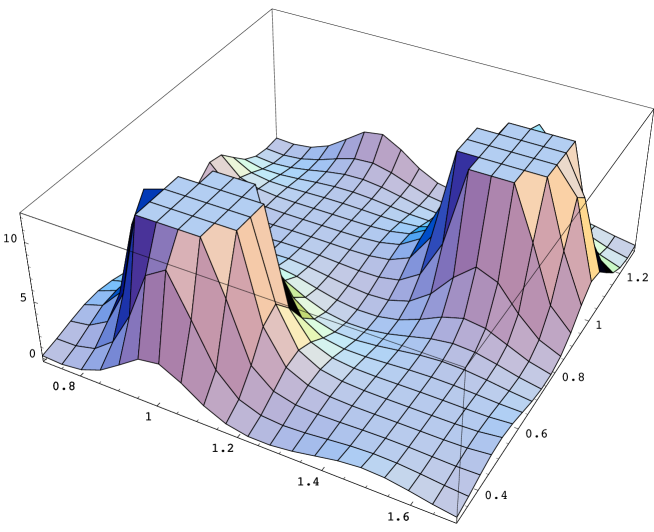
Figure 1: Plot of the density (in units of $1/e^{2}$) associated with the function ${\wp_{t,it}^{\prime}(z)}/{\wp_{t,it}(z)}$ for $t=1$ in the cell $0.7\leq x\leq 1.7$, $0.3\leq y\leq 1.3$. Large values of the density have been clipped.

Numerical integration suggests that for the rationalized charge $q_{\mathrm{torus}}$ associated with this solution ($t>0$ finite) we have

$$q_{\mathrm{torus}}=\frac{e^{2}}{2\pi}\int_{F}\rho_{f_{t}}\,d^{2}x=4\quad(F\mathrel{\mathop{:}}=[0,t]\times[0,t]).$$ (70)

Now, the planar limit of $f_{t}$ is

$$f_{t}(z)\rightarrow\frac{-2}{z}\quad\text{for }t\rightarrow+\infty,$$ (71)

and it is well known that the charge associated with this is

$$q_{\mathrm{plane}}=\frac{e^{2}}{2\pi}\int_{\mathbb{R}^{2}}\rho_{z\mapsto-2/z}\,d^{2}x=2=\frac{1}{2}\,q_{\mathrm{torus}}.$$ (72)

We therefore have the surprising result that, in passing from the torus to the plane, some charge of a vortex can get lost.

An elliptic solution with no flux loss.

That this need not always happen is shown by the example of the density associated with $g(z)=\wp_{t,it}(z)$. Here, the charge in the planar limit is the same as on the torus, namely $=4$.

3.2 Relatives of Olesen’s solution

In [9] Olesen investigated a periodic vortex with charge $q=1$. In our language, this solution is associated with the function $\operatorname{\mathcal{O}}{(z)}$ (equation (63)) for the square lattice $\Omega=\mathbb{Z}t+\mathbb{Z}it$ with $t>0$. In Figure 2 we have plotted this density for $t=1$.

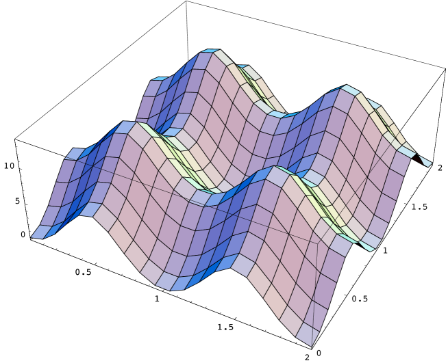
Figure 2: Plot of Olesen’s density (in units of $1/e^{2}$) on a $2\times 2$ grid of cells where the fundamental domain is $[0,1)\times[0,1)$.

We can also look at the density associated with $\operatorname{\mathcal{O}}{(z)}$ on arbitrary tori $\mathbb{C}/(\mathbb{Z}\omega_{1}+\mathbb{Z}\omega_{2})$. For instance, Figure 3 shows the density for a sequence of lattices $\Omega=\mathbb{Z}+\mathbb{Z}it$, where successively $t=.5,.75,1$. Note how the drempel-like structure deforms to the lump of Figure 2 as the rectangle approaches a square. From numerical integration we know that all these vortices have charge $q=1$ and the same appears to be true for tori where the fundamental region is a true parallelogram.

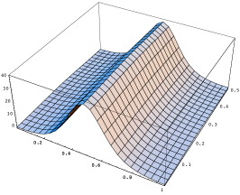
(a) $t=.5$

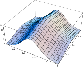
(b) $t=.75$

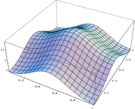
(c) $t=1$

Figure 3: Density (in units of $1/e^{2}$) associated with the function $\operatorname{\mathcal{O}}(z)$ on a sequence of rectangular tori with lattice $\Omega=\mathbb{Z}+\mathbb{Z}it$ for: 3(a) $t=.5$, 3(b) $t=.75$, and 3(c) $t=1$.

What is the planar limit of the density associated with $\operatorname{\mathcal{O}}{(z)}$? It is easy to see that for a square fundamental region, $\operatorname{\mathcal{O}}{(z)}$ approaches a constant as the period lengths tend to positive infinity, that is, in this limit, the associated density approaches $0$. It appears likely that the same is also true for more general fundamental regions.

4 Summary and discussion

In this paper we have studied the Jackiw-Pi model with periodic boundary conditions, which amounts to solving the Liouville equation on the torus. Physically, these solutions describe a two-dimensional periodic lattice of charged vortices with quantized magnetic flux. As first discussed in [1, 2] the existence of vortex solutions requires a delicate tuning of the coupling parameters: the electric charge and the strength of the self-interaction. Surprisingly, it seems that this tuning is not destroyed by quantum fluctuations [21, 6, 18]; on the contrary, the tuning is precisely the condition for which the $\beta$-functions of the model vanish and there is no scale-dependence of the parameters, at least at one-loop order.

On the torus, the spectrum of fluxes of the vortices differs from the planar case; it is richer in that it allows both odd and even integer fluxes. This is possible because periodic functions on the plane do not vanish at infinity, as required for the solutions on the infinite plane. However, it also implies that the limit of the torus to the infinite plane is singular and can change the flux associated with a certain solution. We have presented explicit examples of this phenomenon. This observation may be relevant also in other field theories with soliton solutions, e.g. the Skyrme model as an effective theory for the bound states in QCD.

It is amusing to note that our physical classification of vortices on the torus has a purely mathematical consequence having to do with the geometrical content of the Liouville equation: We can interpret our density $\rho$ as the conformal factor of a metric on a punctured torus, with punctures exactly at the zeros of $\rho$. Our classification theorem then gives all sufficiently smooth metrics of constant Gaussian curvature $K=e^{2}>0$ on punctured tori in explicit form. From our physical arguments in Appendix B it also follows that the properly normalized integral (17) of the conformal factor over the torus is always a non-negative integer.

In reference [22] a topological interpretation of the charge of vortex solutions on the plane was given. It would clearly be interesting to obtain an analogous interpretation for the theory on the torus and we believe that the remarks in Appendix B could constitute the first steps in that direction.

Appendix A Proof of Lemma 2

Here we prove Lemma 2 of Section 2. We only need to supply the proof of the “$\Rightarrow$”-direction; for the “$\Leftarrow$”-direction see [6, 18]. For clarity, let us repeat the statement (in slightly altered notation):

Lemma 2 (“$\Rightarrow$”).

Let $f$ and ${\tilde{f}}$ be non-constant meromorphic functions on the plane and suppose that their associated densities $\rho_{f}$ and $\rho_{{\tilde{f}}}$ are equal: $\rho_{f}=\rho_{{\tilde{f}}}$, where

$$\rho_{f}(z)=\frac{4}{e^{2}}\,\frac{|f^{\prime}(z)|^{2}}{(1+|f(z)|^{2})^{2}},$$ (73)

and analogously for $\rho_{\tilde{f}}$.

Then there exists a matrix

$$\gamma=\begin{bmatrix}a&b\\ c&d\end{bmatrix}\in\mathrm{SU}(2),$$

such that

$${\tilde{f}}(z)=\gamma\cdot f(z)\mathrel{\mathop{:}}=\begin{bmatrix}a&b\\ c&d\end{bmatrix}\cdot f(z)\mathrel{\mathop{:}}=\frac{af(z)+b}{cf(z)+d}.$$ (74)

Proof.

Stereographic projection $\pi:\,S^{2}\rightarrow\widehat{\mathbb{C}}_{w}$ gives a bijection between the sphere $S^{2}$ and the extended complex $w$-plane $\widehat{\mathbb{C}}_{w}$. In this way, the round metric on the sphere, $ds^{2}_{S^{2}}$, induces a distance function $d_{U}$ on $\widehat{\mathbb{C}}_{w}$, for which the distance between two points $w_{1},w_{2}\in\widehat{\mathbb{C}}_{w}$ is given by

$$d_{U}(w_{1},w_{2})=\inf_{\Gamma}\int_{0}^{1}\frac{|\Gamma^{\prime}(t)|}{1+|\Gamma(t)|^{2}}\,dt,$$ (75)

where the infimum is over all curves $\Gamma:\,[0,1]\rightarrow\widehat{\mathbb{C}}_{w}$ with $\Gamma(0)=w_{1}$, $\Gamma(1)=w_{2}$. The orientation preserving isometry group of the sphere, $\mathrm{SO}(3)$, is mapped by $\pi$ to the orientation preserving isometries of $\widehat{\mathbb{C}}_{w}$ equipped with the distance $d_{U}$, which is $\mathrm{PSU(2,\mathbb{C})}$.

For a meromorphic function on the plane $\mathbb{C}_{z}$, define a quasi-distance $d_{f}$ by

$$d_{f}(z_{1},z_{2})\mathrel{\mathop{:}}=d_{U}(f(z_{1}),f(z_{2})).$$ (76)

(We call this a quasi-distance since, although it is positive and satisfies the triangle inequality, it is degenerate in the sense that points $z_{1}$, $z_{2}$ at distance zero are not necessarily equal, but rather satisfy $f(z_{1})=f(z_{2})$.)

The hypothesis of the theorem concerning equality of densities implies that for every $z_{1},z_{2}\in\mathbb{C}_{z}$, we have

$$d_{f}(z_{1},z_{2})=d_{\tilde{f}}(z_{1},z_{2}).$$ (77)

We now define a map $\iota:\,\widehat{\mathbb{C}}_{w}\rightarrow\widehat{\mathbb{C}}_{w}$ by

$$\iota(w)\mathrel{\mathop{:}}={\tilde{f}}(f^{-1}(w)).$$ (78)

First of all, this is well-defined. Indeed, if $f(z_{1})=f(z_{2})=:w$, then the definition (76) implies that $d_{f}(z_{1},z_{2})=0$. Further, equation (77) implies that $d_{\tilde{f}}(z_{1},z_{2})=0$, and, again by definition (76), we obtain ${\tilde{f}}(z_{1})={\tilde{f}}(z_{2})$. Our claim is that $\iota(w)$ is an isometry of $\widehat{\mathbb{C}}_{w}$ equipped with $d_{U}$.

It is surjective, since $f$ and ${\tilde{f}}$ are not constant. Indeed, for any two points $w_{1},w_{2}\in\mathbb{C}_{w}$, we have

$$d_{U}(\iota(w_{1}),\iota(w_{2}))=d_{\tilde{f}}(f^{-1}(w_{1}),f^{-1}(w_{2}))=d_{f}(f^{-1}(w_{1}),f^{-1}(w_{2}))=d_{U}(w_{1},w_{2}).$$ (79)

Also, $\iota$ is orientation-preserving since $f$ is meromorphic.

Hence, ${\tilde{f}}=T(f)$ for some orientation preserving isometry $T$ of $\widehat{\mathbb{C}}_{w}$, that is $T\in\mathrm{PSU(2,\mathbb{C})}$, whence there is a matrix

$$\gamma=\begin{bmatrix}a&b\\ c&d\end{bmatrix}\in\mathrm{SU}(2),$$ (80)

such that

$${\tilde{f}}=\gamma\cdot f.$$ (81)

∎

Remark.

It is clear that this lemma can be used for determining the precise structure of the moduli space of self-dual static vortices of the Jackiw-Pi model on the plane. For, according to Horvathy and Yera [8], any such vortex with flux $\Phi=4\pi N/e$ is given by a density $\rho_{f}$, where $f$ is a rational function

$$f(z)=\frac{P(z)}{Q(z)},\quad\deg{P}<\deg{Q}=N.$$ (82)

Therefore, every such solution has $4N$ moduli but, obviously, they are not all independent. Rather, by our result, the moduli space is some kind of quotient

$$\mathbb{C}^{2N}/\mathrm{PSU(2,\mathbb{C})}.$$

The invariant theory of $\mathrm{PSU(2,\mathbb{C})}$ is well-studied, see e.g. [23]. We leave the problem of working out the physical implications in detail for the future [24].

Appendix B Quantization of flux

We comment here on the quantization of flux of static vortex solutions of the Jackiw-Pi model.

For the theory on the plane, this quantization is best seen a posteriori from the results of Horvathy and Yera [8]. For the time being, an analogous result on the torus is, however, not available [24]. That is, given a solution from the classification Theorem 1 we cannot say at the moment, without resorting to numerical integration, what its associated flux is.

Therefore, we now proceed to give a more general argument supporting the claim that the flux is also quantized in the torus case.

The boundary conditions of the Jackiw-Pi model on a spacetime of the form $\mathbb{R}\times T^{2}$, where $T^{2}=\mathbb{C}/\Omega$ for some lattice $\Omega$, are somewhat subtle. Naively, one would write the gauge potential $A$ as a 1-form on the torus, which would lead to

$$\int_{T^{2}}B=\int_{T^{2}}dA=\int_{\partial T^{2}=\emptyset}A=0,$$ (83)

in contradiction to the solutions with a non-vanishing magnetic flux. The resolution to this puzzle is of course analogous to the Dirac monopole, where we need multiple gauge patches to describe the solution; in other words, $A$ in reality is a section of a bundle.

However, because we are dealing with a torus, we can also pull back the gauge connection to the plane, where the gauge potential can be written as a 1-form. The boundary conditions are then implemented by periodicity of the fields $\rho$, $E$, and $B$, which translates to the equations

$$\begin{split}\Psi(x+\omega_{i})=e^{i\theta_{i}(x)}\Psi(x),\\ A(x+\omega_{i})=A(x)+d\theta_{i}(x),\\ \end{split}$$ (84)

where $\Omega=\mathbb{Z}\omega_{1}+\mathbb{Z}\omega_{2}$, that is, our lattice is generated by $\omega_{1}$ and $\omega_{2}$.

Now we can use gauge transformations in the plane to set the phase $\theta_{2}$ to zero, and then we are left with a single phase $\theta_{1}$. It is easy to show that under translation by $\omega_{2}$ we have

$$e^{i\theta_{1}(x)}=e^{i\theta_{1}(x+\omega_{2})},$$ (85)

and thus $\theta_{1}(x+\omega_{2})=\theta_{1}(x)+2\pi n$. This means that the total magnetic flux through the torus is

$$\int_{F}B=\int_{F}dA=\int_{\partial F}A,$$ (86)

where

$$F\mathrel{\mathop{:}}=\{t_{1}\omega_{1}+t_{2}\omega_{2}\,|\,0\leq t_{1},t_{2}<1\}$$ (87)

is the fundamental domain of the torus in the plane. The boundary integral is the integral along the parallelogram where the two sides in the direction of $\omega_{1}$ cancel, due to periodicity of $A$ in $\omega_{2}$. However, the sides in the direction of $\omega_{2}$ do not cancel, due to the non-periodicity caused by $\theta_{1}$. The difference between the two sides is given by

$$\int_{\partial F}A=\int_{0}^{\omega_{2}}d\theta_{1}=2\pi n.$$ (88)

Therefore, the total magnetic flux is quantized in units of $2\pi$. The topology of the principal $\mathrm{U}(1)$ gauge bundle over the torus is that of a twisted 3-torus with twist $n$.

Appendix C Elliptic functions of the second kind

For easy reference we repeat here the results of [14], p. 154 concerning elliptic functions of the second kind (=multiplicative quasi-elliptic functions) specialized to the needs of the present paper (see also [25, 26]).

Definition.

Let $\Omega=\mathbb{Z}\omega_{1}+\mathbb{Z}\omega_{2}$ be a lattice. A function $f$ which is meromorphic in the plane is said to be an elliptic function of the second kind with multipliers of unit modulus, if there exist complex numbers $\mu_{1},\mu_{2}$, with $|\mu_{1}|,|\mu_{2}|=1$, such that

$$f(z+\omega_{i})=\mu_{i}\,f(z)\quad(i=1,2).$$ (89)

Theorem (Lu [14]).

A function $f$ which is meromorphic in the plane is an elliptic function of the second kind with multipliers $\mu_{1},\mu_{2}$ of unit modulus if and only if there are complex constants

$$a_{0},\dots,a_{n}\in\mathbb{C},$$ (90)

and parameters

$$z_{1},\dots,z_{n}\in\{t_{1}\omega_{1}+t_{2}\omega_{2}\,|\,0\leq t_{1},t_{2}<1\},$$ (91)

such that

$$f(z)=\left[a_{0}+\sum_{k=1}^{n}a_{k}\frac{d^{k}\zeta}{dz^{k}}(z-z_{0})\right]\frac{\sigma(z-z_{0})^{n}}{\prod_{k=1}^{n}\sigma(z-z_{k})}\,e^{\lambda\,z},$$ (92)

where

$$\lambda=\frac{1}{\pi i}\,(\gamma_{2}\,\eta_{1}-\gamma_{1}\,\eta_{2}),$$ (93)

and

$$z_{0}=\frac{1}{2n\pi i}\,(\gamma_{2}\,\omega_{1}-\gamma_{1}\,\omega_{2})+\frac{1}{n}\sum_{k=1}^{n}z_{k}.$$ (94)

Here, $\eta_{i}\mathrel{\mathop{:}}=\zeta_{\omega_{1},\omega_{2}}(\omega_{i}/2)$ and $\gamma_{i}\mathrel{\mathop{:}}=\log{\mu_{i}}$ ($i=1,2$). (The branch of $\log{\mu_{i}}$ can be chosen arbitrarily.)

References

• [1] R. Jackiw and S.-Y. Pi, “Classical and quantal nonrelativistic Chern-Simons theory,” Phys. Rev. D42 (1990) 3500–3513.
• [2] R. Jackiw and S.-Y. Pi, “Soliton Solutions to the Gauged Nonlinear Schrodinger Equation on the Plane,” Phys. Rev. Lett. 64 (1990) 2969–2972.
• [3] R. Jackiw and S.-Y. Pi, “Selfdual Chern-Simons solitons,” Prog. Theor. Phys. Suppl. 107 (1992) 1–40.
• [4] P. A. Horvathy, “Lectures on (abelian) Chern-Simons vortices,” arXiv:0704.3220 [hep-th].
• [5] P. A. Horvathy and P. Zhang, “Vortices in (abelian) Chern-Simons gauge theory,” Phys. Rept. 481 (2009) 83–142, arXiv:0811.2094 [hep-th].
• [6] M. O. de Kok and J. W. van Holten, “The Role of Conformal Symmetry in the Jackiw-Pi Model,” Nucl. Phys. B805 (2008) 545–558, arXiv:0806.3358 [hep-th].
• [7] J. Liouville, “Sur l’équation aux différences partielles $\frac{d^{2}\log\lambda}{dudv}\pm\frac{\lambda}{2a^{2}}=0$,” J. Math. Pures et Appl. Tome XVIII (1853) 71–72.
• [8] P. A. Horvathy and J. C. Yera, “Vortex solutions of the Liouville equation,” Lett. Math. Phys. 46 (1998) 111–120, arXiv:hep-th/9805161.
• [9] P. Olesen, “Soliton condensation in some selfdual Chern-Simons theories,” Phys. Lett. B265 (1991) 361–365.
• [10] J. Kazdan and F. Warner, “Curvature functions for compact 2-manifolds,” Ann. of Math. (2) 99 (1974) 14–47.
• [11] H. Bateman, Partial Differential Equations of Mathematical Physics. Dover Publications, 1944.
• [12] T. Tao, “An explicitly solvable nonlinear wave equation.” Blog entry, http://terrytao.wordpress.com/2009/01/22/.
• [13] A. M. Arthurs, J. Clegg, and A. K. Nagar, “On the Solution of the Liouville Equation over a Rectangle,” J. of Appl. Math. and Stoch. Analysis 9 (1996) 57–67.
• [14] J. K. Lu, Boundary Value Problems for Analytic Functions. World Scientific, 1993.
• [15] L. V. Ahlfors, Complex Analysis. McGraw-Hill, third ed., 1979.
• [16] E. Whittaker and G. N. Watson, A Course of Modern Analysis. Cambridge Univ. Press, fourth ed., 1927.
• [17] M. O. de Kok. Unpublished work, private communication by P. A. Horvathy.
• [18] M. O. de Kok, Broken Symmetries in Field Theory. Doctoral thesis, Leiden University, 2008.
• [19] P. Olesen, “Vacuum structure of the electroweak theory in high magnetic fields,” Phys. Lett. B268 (1991) 389–393.
• [20] C. L. Siegel, Topics in Complex Function Theory, Vol. I: Elliptic Functions and Uniformization Theory. Wiley–Interscience, 1969.
• [21] O. Bergman and G. Lozano, “Aharonov-Bohm scattering, contact interactions and scale invariance,” Ann. Phys. 229 (1994) 416–427, arXiv:hep-th/9302116.
• [22] P. A. Horvathy, “Topology of non-topological Chern-Simons vortices,” Lett. Math. Phys. 49 (1999) 67–70, arXiv:hep-th/9903116.
• [23] T. A. Springer, “On the invariant theory of $\mathrm{SU}_{2}$,” Nederl. Akad. Wetensch. Indag. Math. 42 (1980) no. 3, 339.
• [24] N. Akerblom, G. Cornelissen, G. Stavenga, and J. W. van Holten. In preparation.
• [25] A. R. Forsyth, Theory of Functions of a Complex Variable. University Press, Cambridge (UK), 1893.
• [26] Math. Soc. of Japan and K. Itō (eds.), Encyclopedic Dictionary of Mathematics. MIT Press, Cambridge, Mass., second ed., 1987.