Berry’s phase and the anomalous velocity of Bloch wavepackets

Abstract

The semiclassical equations of motion for a Bloch electron include an anomalous velocity term analogous to a $k$-space “Lorentz force”, with the Berry connection playing the role of a vector potential. By examining the adiabatic evolution of Bloch states in a monotonically-increasing vector potential, I show that the anomalous velocity can be explained as the difference in the Berry’s phase acquired by adjacent Bloch states within a wavepacket.

When inversion or time-reversal symmetry is broken, the semiclassical motion for a Bloch electron is known to contain an additional non-vanishing term analogous to the Lorentz force in momentum-space:

$$\dot{r}=\frac{1}{\hbar}\nabla_{k}E_{k}+\dot{k}\times\left(\nabla_{k}\times\mathcal{A}_{k}\right).$$ (1)

Here, $k$ is the reduced wave-vector, $E_{k}$ is the band energy, $\nabla_{k}$ denotes a $k$-space derivative, and $\mathcal{A}_{k}$ is defined by

$$\vec{\mathcal{A}}_{k}=\frac{1}{i}\int_{\Omega}\!d^{d}\!r\,u_{k}^{*}(r)\nabla_{k}u_{k}(r),$$ (2)

with the integral taken over the unit cell $\Omega$ and $u_{k}(r)$ denoting the Bloch function. The “anomalous velocity”—the second term on the right hand side of (1)—was originally derived by Karplus and LuttingerKL in their explanation of the extraordinary Hall coefficients of ferromagnetic materials, based on a careful examination of wavepacket dynamics. Subsequently, Chang and Niu re-derived the anomalous velocity using an effective-Lagrangian technique, and pointed out that $\vec{\mathcal{A}}_{k}$ is the important quantity known as the Berry connection ChangNiu .

In its original context, the Berry connection describes the gauge structure of a quantum state as it undergoes adiabatic evolution, following a trajectory $\vec{\lambda}(t)$ in some parameter space of the system Hamiltonian $H(\lambda(t))$. The line integral of the Berry curvature, taken over $\vec{\lambda}(t)$, yields “Berry’s phase”—an additional phase acquired by the quantum state during the adiabatic process Berry . As first appreciated by Simon Simon , the Berry connection also emerges within Bloch systems, in a manner that appears to be quite different: the reduced wave-vector $k$ serves as the “parameter” for the reduced Hamiltonian $H(k)$, and $\vec{\mathcal{A}}_{k}$ describes the gauge structure of the Bloch functions $u_{k}(r)$ within the Brillouin zone. (In particular, the integral of $\vec{\mathcal{A}}_{k}$ along the boundary of a two-dimensional Brillouin zone yields the TKNN number, which equals the index of the integer quantum Hall effect TKNN .)

I would like to present a derivation of the anomalous velocity that clarifies its relationship with adiabatic quantum evolution, the context in which the Berry connection first arose. One virtue of this derivation is that it provides a simple geometrical explanation of why the anomalous velocity involves the $k$-space curl of the Berry connection (the “Berry curvature”). The idea is simple: a small DC electric field can be represented by a constant vector potential that increases monotonically with time. Each Bloch state undergoes adiabatic evolution in this vector potential, and acquires a Berry’s phase. Each Bloch component of a wavepacket undergoes a different $k$-space trajectory, and acquires a different Berry’s phase. The resulting Berry’s phase differences, characterized by the Berry curvature, conspire to induce the anomalous term in the velocity of the wavepacket as a whole.

For simplicity of presentation, I will ignore the magnetic field (whose presence does not alter the final results). A Hamiltonian for a Bloch electron subjected to an additional small electric field $\mathcal{E}\hat{x}$ is

$$H^{\prime}=-\frac{\hbar^{2}}{2m}\nabla^{2}+V(r)-e\mathcal{E}x,$$ (3)

where $V(r)$ is the lattice potential, which can break inversion symmetry. A gauge transformation $\phi\rightarrow\phi-(1/c)\partial_{t}\Lambda$ and $A\rightarrow A+\nabla\Lambda$, where $\Lambda=-\mathcal{E}cxt$, yields the equivalent periodic time-dependent Hamiltonian

$$H(t)=\frac{\hbar^{2}}{2m}\left[-i\nabla+\frac{et}{\hbar}\vec{\mathcal{E}}\,\right]^{2}+V(r).$$ (4)

The quantum states of the new Hamiltonian have an extra phase factor of $\exp(-ie\mathcal{E}xt/\hbar)$, which is the same for all states and therefore irrelevant.

As pointed out by KittelKittel , $H$ now has the form of a reduced Hamiltonian:

$$H(t) = H(\vec{q}(t)),\qquad\vec{q}(t)=\frac{et}{\hbar}\,\vec{\mathcal{E}},$$ (5)

$$H(k) \equiv \frac{\hbar^{2}}{2m}\left[-i\nabla+\vec{k}\right]^{2}+V(r).$$ (6)

This allows us to describe the effects of the electric field in terms of adiabatic evolution. Similar considerations were used by Zak in a related one-dimensional modelZak .

The Bloch states are eigenstates of $H(\vec{k})$ with band energies $E(k)$ (suppressing the irrelevant band index):

$$H(k)\,u_{k}(r)=E(k)\,u_{k}(r).$$ (7)

It is easily seen that

$$H(k^{\prime})\left[u_{k^{\prime}+k}(r)\,e^{ikr}\right]=E(k^{\prime}+k)\,\left[u_{k^{\prime}+k}(r)\,e^{ikr}\right].$$ (8)

Therefore, at each time $t$ the Hamiltonian $H(q(t))$ possesses a set of instantaneous eigenstates $u_{q(t)+k}(r)\,e^{ikr}$. (For $t=0$, these are the usual Bloch states.) If the electric field $\mathcal{E}$ is weak, the change is adiabatic.

Suppose we have the initial state

$$\psi(r,t=0)=u_{k}(r)\,e^{ikr}.$$ (9)

According to Berry’s theorem Berry , the state at time $t$ is

$$\psi(t)=u_{k(t)}\,e^{ikr}\,\exp\left[-\frac{i}{\hbar}\int_{0}^{t}dt^{\prime}E(k(t^{\prime}))\right]\,e^{i\gamma_{k}(t)},$$ (10)

where $k(t)\equiv k+q(t)$. Berry’s phase, $\gamma_{k}(t)$, is given by

$$\gamma_{k}(t) = i\int d\vec{q}^{\prime}\cdot\left[\int_{\Omega}d^{d}r\,\left(u_{q^{\prime}+k}e^{ikr}\right)^{*}\nabla_{q^{\prime}}\left(u_{q^{\prime}+k}e^{ikr}\right)\right]$$ (11)

$$= -\int_{k(0)}^{k(t)}d\vec{k}^{\prime}\cdot\vec{\mathcal{A}}_{k^{\prime}},$$

with the integral taken over the trajectory of $k(t)$.

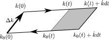
Figure 1: $k$-space line integrals giving rise to the Berry’s phases in equation (16).

Now consider a wavepacket composed of Bloch states, initially centered on the Bloch state with $k=k_{0}$:

$$\psi(r,0) = \sum_{k}f(|k-k_{0}|)\,u_{k}(r)\,e^{ikr}$$ (12)

$$= e^{ik_{0}r}\sum_{k}f(|\Delta k|)\,u_{k}(r)\,e^{i\Delta k\cdot r},$$ (13)

where $\Delta k=k-k_{0}$ and $f$ is some envelope function. From (10) and (11), the wavepacket at time $t$ is

$$\psi(r,t)=e^{ik_{0}r}\sum_{k}f(|\Delta k|)\,u_{k(t)}(r)\,\\ \times e^{i\Delta k\cdot r}\exp\left[-\frac{i}{\hbar}\int_{0}^{t}dt^{\prime}E(k(t^{\prime}))\right]\,e^{i\gamma_{k}(t)}.$$ (14)

Note that $k(t)-k_{0}(t)=\Delta k$ is time-independent. Comparing (14) to (13), we observe displacements in both $r$ and $k$. The $k$-space displacement is simply $q(t)$. The $r$-space displacement is determined by the phase factors on the last line of (14), which should have the form

$$(\textrm{overall phase factor})\times\exp\left[i\Delta k\cdot r(t)\right],$$

where the overall phase factor comes from the phase of the central wavepacket $k_{o}(t)$ and the second term comes from the phase difference between $k(t)$ and $k_{o}(t)$.

From these considerations, we see that the phase differences between $k$ and $k_{0}$ which arise from the band energies yield the usual group velocity:

$$\Delta k\cdot\vec{v}_{g} = \frac{d}{dt}\left\{\frac{1}{\hbar}\int_{0}^{t}dt^{\prime}\left[E(k(t^{\prime}))-E(k_{0}(t^{\prime}))\right]\right\}$$ (15)

$$= \Delta k\cdot\left[\frac{1}{\hbar}\nabla_{k}E(k_{0}(t))\right].$$ (16)

I now claim that the Berry’s phase differences give the anomalous velocity:

$$\Delta k\cdot\vec{v}_{a}=\frac{d}{dt}\left\{\int_{k(0)}^{k(t)}\!d\vec{k}^{\prime}\cdot\vec{\mathcal{A}}_{k^{\prime}}-\int_{k_{0}(0)}^{k_{0}(t)}\!d\vec{k}^{\prime\prime}\cdot\vec{\mathcal{A}}_{k^{\prime\prime}}\right\}.$$ (17)

To prove this, observe that the line integrals are taken over the top and bottom segments of the parallelogram in Fig. 1. When $\Delta k$ is sufficiently small, integrals $\int d\vec{k}^{\prime}\cdot\vec{\mathcal{A}}_{k^{\prime}}$ over the side segments become negligible; then the two separate line integrals can be replaced with a single edge integral, taken clockwise around the boundary $\Gamma(t)$ of the paralleogram:

$$\Delta k\cdot\vec{v}_{a} \approx \frac{d}{dt}\left\{\oint_{\Gamma(t)}d\vec{k}^{\prime}\cdot\vec{\mathcal{A}}_{k^{\prime}}\right\}$$ (18)

$$= -\frac{d}{dt}\left\{\int_{a(t)}da\cdot\left(\nabla_{k}\times\vec{\mathcal{A}}_{k^{\prime}}\right)\right\}.$$ (19)

In time $dt$, the edge advances by $\dot{k}dt$, and the additional area (grey region in Fig. 1) is $(\dot{k}\times\Delta k)dt$. Thus,

$$\Delta k\cdot\vec{v}_{a} = \left(\nabla_{k}\times\vec{\mathcal{A}}_{k_{0}}\right)\cdot\left(\Delta k\times\dot{k}\right)$$ (20)

$$= \Delta k\cdot\left(\dot{k}\times\nabla_{k}\times\vec{\mathcal{A}}_{k_{0}}\right).$$ (21)

This is precisely the anomalous velocity given in (1).

I am grateful to P. A. Lee for helpful discussions.

References

(1) R. Karplus and J. M. Luttinger, Phys. Rev. Lett. 95, 1154
(1954).
(2) M. C. Chang and Q. Niu, Phys. Rev. Lett. 75, 1348
(1995), Phys. Rev. B 53, 7010 (1996).
(3) M. V. Berry, Proc. R. Soc. A392, 45 (1984).
(4) B. Simon, Phys. Rev. Lett. 51, 2167 (1983).
(5) D. J. Thouless, M. Kohmoto, M. Nightingale, and M. den
Nijs, Phys. Rev. Lett. 49, 405 (1982).
(6) C. Kittel, Quantum Theory of Solids (Wiley, New
York, 1963), p. 190.