Increasing the statistical significance of entanglement detection in experiments

Abstract

Entanglement is often verified by a violation of an inequality like a Bell inequality or an entanglement witness. Considerable effort has been devoted to the optimization of such inequalities in order to obtain a high violation. We demonstrate theoretically and experimentally that such an optimization does not necessarily lead to a better entanglement test, if the statistical error is taken into account. Theoretically, we show for different error models that reducing the violation of an inequality can improve the significance. Experimentally, we observe this phenomenon in a four-photon experiment, testing the Mermin and Ardehali inequality for different levels of noise. Furthermore, we provide a way to develop entanglement tests with high statistical significance.

Introduction — Quantum theory is a statistical theory, predicting in general only probabilities for experimental results. Consequently, in most experiments observing quantum effects, several copies of a quantum state are generated and individually measured to determine the desired probabilities. As only a finite number of states can be generated, this leads to an unavoidable statistical error. The particularly low generation rate in certain experiments demands a careful statistical treatment; a fact that is well known from particle physics hepandastro ; feldman .

In quantum information processing, many of today’s experiments aim at the generation of entanglement, which is considered to be a central resource hororeview ; review . So far, entanglement of up to ten qubits has been achieved using trapped ions or photons experiments ; luexp . For the experimental verification of entanglement, often inequalities for the correlations — such as Bell inequalities or entanglement witnesses — are used review , in which a violation indicates entanglement. The maximization of this violation has been investigated in detail, cf. Refs. review ; EWoptimization . In fact, making such inequalities more sensitive is a crucial step in order to allow advanced experiments with more particles.

In this paper we demonstrate theoretically and experimentally that such an optimization does not necessarily lead to a better entanglement test, if the statistical nature of quantum theory is taken into account. It was already noted gill that, when aiming at ruling out local realism, highly entangled states do not necessarily deliver a stronger test than weakly entangled states, but this does not answer the question which inequality to use for a given state and it remains unclear how to apply it to actual error models used in experiments. Also, most of the different entanglement detection methods compared in Ref. altepeter cannot be applied to multiparticle systems.

Theoretically, we show for different error models that decreasing the violation of an inequality can improve the significance. Also, we demonstrate this phenomenon in a four-photon experiment, measuring the Mermin and the Ardehali inequality. We find that the former inequality leads to a higher significance than the latter, despite a lower violation. Finally, we discuss the physical origin of this phenomenon and provide methods to construct entanglement tests with a high statistical significance.

Statement of the problem — A witness $\mathcal{W}$ is an observable which has a non-negative expectation value on all separable states (i.e., states which can be written as a mixture of product states, $\varrho=\sum_{k}p_{k}|a_{k},b_{k}\rangle\langle a_{k},b_{k}|$ with some probabilities $p_{k}$). Hence, a negative expectation value of a witness signals entanglement. Similarly, a Bell inequality $\langle{\mathcal{B}}\rangle\leq C_{\rm lhv}$, where $\mathcal{B}$ is a sum of certain correlation terms, holds if the measurement outcomes can originate from a local hidden variable (LHV) model. As separable states allow a description by LHV models, a violation of a Bell inequality implies the presence of entanglement.

In both cases, we define $\mathcal{V}$ as the violation of the corresponding inequality. That is, for a witness we have $\mathcal{V}(\mathcal{W})=-\langle{\mathcal{W}}\rangle$ while for a Bell inequality $\mathcal{V}(\mathcal{B})=\langle{\mathcal{B}}\rangle-C_{\rm lhv}.$ Then, the significance of an entanglement test can be defined as

$$\mathcal{S}=\frac{\mathcal{V}}{\mathcal{E}}$$ (1)

where $\mathcal{E}$ is the statistical error for the experiment. Clearly, $\mathcal{E}$ depends on the particular experimental implementation and on the error model used. Nevertheless, in any experiment $\mathcal{S}$ is a well characterized quantity; its notion is widely used in the literature, when the violation is expressed in terms of “standard deviations”, also in other fields of physics hepandastro .

Previously, much effort has been devoted to improving entanglement tests in order to achieve a higher violation. For instance, for entanglement witnesses a mature theory how to optimize witnesses has been developed EWoptimization . Here, for a given witness $\mathcal{W}$ one tries to find a positive operator $P$, such that $\mathcal{W}^{\prime}=\mathcal{W}-P$ is still a witness. In order to have a more significant result, however, one can either increase $\mathcal{V}$ in Eq. (1) or decrease $\mathcal{E}.$ It is a central result of this paper that decreasing $\mathcal{E}$ is often superior.

Variance as the error — Let us first consider a simple model, in which we take the square root of the variance as the error of a witness,

$$\mathcal{E}(\mathcal{W})=\Delta(\mathcal{W})=\sqrt{\langle{\mathcal{W}^{2}}\rangle-\langle{\mathcal{W}}\rangle^{2}}.$$ (2)

An experimentally relevant model will be discussed below. This simple model already demonstrates that the standard optimization of witnesses is often not the appropriate approach to increase the significance:

Observation. Let $\varrho=|\psi\rangle\langle\psi|$ be a pure state detected by the witness $\mathcal{W}.$ Then, one can always increase the significance of $\mathcal{W}$ at the expense of optimality (i.e., by adding a positive operator). With this method one can make the significance arbitrarily large.

Namely, one needs to find a positive observable $P$, such that $|\psi\rangle$ is an eigenstate of $\mathcal{W}^{\prime}=\mathcal{W}+P$; then the error vanishes. Indeed, such a $P$ can be found (see Appendix).

Multi-photon experiments — Let us now consider a realistic situation, in which other and more specific error models are used. As our later implementation uses multi-photon entanglement, we concentrate on this type of experiments but our ideas can also be applied to other implementations, such as trapped ions.

The basic experimental quantities are the numbers of detection events $n_{i}$ of the different detectors $i$. From these data, all other quantities such as correlations or mean values of observables are derived.

In the standard error model for photonic experiments luexp ; james , the counts are assumed to be distributed according to a Poissonian distribution, whose mean value is given by the observed value. That is, for a certain measurement outcome $i$ one sets the mean value as $\langle{n_{i}}\rangle=n_{i}$ and the error as $\mathcal{E}(n_{i})=\sqrt{n_{i}}$ (being the standard deviation of a Poissonian distribution). In general, for a function $f=f(n_{i})$ of several counts, Gaussian error propagation is applied to obtain the error (see below).

To give an example, consider a two-qubit correlation

$$\mathcal{M}=\alpha Z_{1}Z_{2}+\beta Z_{1}\openone_{2}+\gamma\openone_{1}Z_{2}.$$ (3)

Here and in the following, $Z_{k}$ (or $\openone_{k}$) denotes the Pauli matrix $\sigma_{z}$ (or the identity matrix) acting on the $k$th qubit and tensor product symbols are omitted. $\langle{\mathcal{M}}\rangle$ can be determined by measuring in the common eigenbasis of all three terms in $\mathcal{M}$, i.e., by projecting onto $|00\rangle,|01\rangle,|10\rangle$ and $|11\rangle$. Repeating this with many copies of the state will lead to count numbers $n_{kl}$ with $k,l=0$ or $1$ and to count rates $p_{kl}=n_{kl}/n_{\rm tot},$ where $n_{\rm tot}=n_{00}+n_{01}+n_{10}+n_{11}$ is the total number of events. The mean value $\langle{\mathcal{M}}\rangle$ can be written as a linear combination of $p_{kl}$, namely $\langle{\mathcal{M}}\rangle=\lambda_{00}p_{00}+\lambda_{01}p_{01}+\lambda_{10}p_{10}+\lambda_{11}p_{11}$ with $\lambda_{00}=\alpha+\beta+\gamma,\lambda_{01}=-\alpha+\beta-\gamma,\lambda_{10}=-\alpha-\beta+\gamma,$ and $\lambda_{11}=\alpha-\beta-\gamma$. Then, according to Gaussian error propagation, the squared error is given by remarkjames

$$\mathcal{E}(\mathcal{M})^{2}={\sum_{k,l}\Big{[}\frac{\partial\langle{\mathcal{M}}\rangle}{\partial{n_{kl}}}\Big{]}^{2}\mathcal{E}(n_{kl})^{2}}={\sum_{k,l}\Big{[}\frac{\lambda_{kl}}{n_{\rm tot}}-\frac{\langle{\mathcal{M}}\rangle}{n_{\rm tot}}\Big{]}^{2}n_{kl}.}$$ (4)

Let us finally discuss the underlying assumptions of this error model. The first main assumption is that the $n_{kl}$ are Poisson distributed and their errors are uncorrelated. This is well motivated by the experimental observations. Moreover, Gaussian error propagation stems from a Taylor expansion of the function $f$. Finally, if one interprets the standard deviation as a confidence interval, one tacitly assumes that the distribution is Gaussian, as for other distributions the connection is not so direct. If the number of events for all detectors is sufficiently large (e.g. $n_{kl}\gtrsim 10$), however, the Poissonian distribution is approximated well by a Gaussian distribution.

Bell inequalities for four particles — Let us now discuss the Mermin and Ardehali inequality as experimentally relevant examples. First, we consider

$$\mathcal{B}_{\rm M}=\> X_{1}X_{2}X_{3}X_{4}-[X_{1}X_{2}Y_{3}Y_{4}+\!\mbox{ perm.}]+\>Y_{1}Y_{2}Y_{3}Y_{4},$$ (5)

where the bracket $[\dots]$ is meant as a sum over all permutations of $X_{1}X_{2}Y_{3}Y_{4}$ that yield distinct operators. For states allowing an LHV description, the Mermin inequality $\langle{\mathcal{B}_{\rm M}}\rangle\leq 4$ holds Mermin . We wrote $\mathcal{B}_{\rm M}$ with the Pauli matrices as observables, since they are used later, however, one might replace them by arbitrary dichotomic measurements.

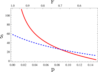
Figure 1: Significance $\mathcal{S}$ for the Mermin (red, solid) and the Ardehali inequality (blue, dashed) for bit-flip noise. On the horizontal axes, we show the bit-flip probability and the corresponding fidelity with respect to a perfect GHZ state. We assumed that the experimenter prepares 8000 instances of a GHZ state and chooses either to measure the eight terms of the Mermin inequality (each term with 1000 realizations of the state) or the 16 terms of the Ardehali inequality with 500 states per correlation term. See text for further details.

Second, we consider the Ardehali inequality $\langle\mathcal{B}_{\rm A}\rangle\leq 2\sqrt{2}$ Ardehali , where

$$\mathcal{B}_{\rm A} =\left(X_{1}X_{2}X_{3}A_{4}+X_{1}X_{2}X_{3}B_{4}\right.$$

$$-[X_{1}Y_{2}Y_{3}A_{4}+\mbox{ perm.}]-[X_{1}Y_{2}Y_{3}B_{4}+\mbox{ perm.}]$$

$$-[X_{1}X_{2}Y_{3}A_{4}+\mbox{ perm.}]+[X_{1}X_{2}Y_{3}B_{4}+\mbox{ perm.}]$$

$$\left.+Y_{1}Y_{2}Y_{3}A_{4}-Y_{1}Y_{2}Y_{3}B_{4}\right)/{\sqrt{2}}.$$ (6)

Here, the sums in square brackets include all distinct permutations on the first three qubits. We set $A_{4}=\left(X_{4}+Y_{4}\right)/\sqrt{2}$ and $B_{4}=\left(X_{4}-Y_{4}\right)/\sqrt{2}$, but again, the observables can remain arbitrary remarkidentical .

The Mermin and Ardehali inequality reveal the non-local correlations of the four-qubit GHZ state,

$$|GHZ_{4}\rangle=\frac{1}{\sqrt{2}}(|0000\rangle+|1111\rangle).$$ (7)

For this state we have $\langle{\mathcal{B}_{\rm M}}\rangle=\langle{\mathcal{B}_{\rm A}}\rangle=8.$ As the bound for LHV models for the Ardehali inequality is smaller, the violation $\mathcal{V}$ is larger. This may lead to the opinion that the Ardehali inequality is “better” than the Mermin inequality for the state $|GHZ_{4}\rangle.$

However, this belief is easily shattered, if the significance $\mathcal{S}$ is considered as the relevant figure of merit. This can be seen directly from Eq. (4). The GHZ state is an eigenstate for each of the correlation measurements in the Mermin inequality (they are so-called stabilizing operators of the GHZ state). Hence, if the Mermin inequality for a perfect GHZ state is measured, we have in the last term of Eq. (4) for each case $k,l$ either $\lambda_{kl}=\langle{\mathcal{M}}\rangle$ (since the mean value is an eigenvalue) or $n_{kl}=0,$ hence $\mathcal{E}(\mathcal{M})$ vanishes. The Ardehali inequality, however, does not contain stabilizer terms and the error remains finite.

For an experimental application it is important that the Mermin inequality leads to a higher significance than the Ardehali inequality, even if noise is introduced remarkimportant . To see this, we considered bit-flip noise, which can easily be simulated in experiment. Therefore, we used a perfect GHZ state whose qubits are locally affected by the bit-flip operation $f$ with probability $p$, i.e. $f(\varrho_{i})=(1-p)\varrho_{i}+pX_{i}\varrho_{i}X_{i}$ for each qubit $i$. In Fig. 1, we plotted the significance $\mathcal{S}$ versus the fidelity $F$ of the noisy state w.r.t. a perfect GHZ state, i.e. $F=\langle{GHZ_{4}}|\varrho_{exp}|{GHZ_{4}}\rangle$, and versus the bit-flip probability $p$. For $F\geq 0.70$ the Mermin inequality is more significant (for the 6-qubit versions of these inequalities Mermin ; Ardehali , this changes to $F\geq 0.40$). As can be seen from Eq. (4), the fact that one witness is more significant than the other one is independent of the total particle number. Moreover, a calculation for white noise yields very similar values ($F\geq 0.72$ for 4 qubits, $F\geq 0.41$ for 6 qubits). This suggests that the effect does not depend on details of the noise. Note that the threshold value for white noise vanishes exponentially fast for an increasing number of qubits.

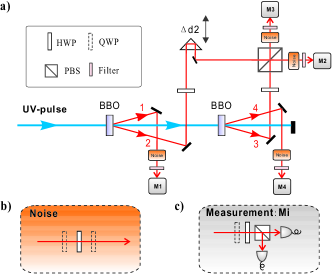
Figure 2: Scheme of the experimental setup. a. The setup to generate the required four-photon GHZ state. Femtosecond laser pulses ($\approx$ 200 fs, 76 MHz, 788 nm) are converted to ultraviolet pulses through a frequency doubler LiB₃O₅ (LBO) crystal (not shown). The pulses go through two main $\beta$-barium borate (BBO) crystals (2 mm), generating two pairs of photons. The observed two-fold coincidence count rates are about $1.6\times 10^{4}/$s with a visibility of 96% (94%) in the $H/V$ ($+/-$) basis. b. Setup for engineering the bit-flip noise. c. The measurement setup.

Experimental setup — Spontaneous down conversion has been used to produce the desired four-photon state [see Fig. 2(a)]. With the help of polarizing beam splitters (PBSs), half-wave plates (HWPs) and conventional photon detectors, we prepare a four-qubit GHZ state, where $\left|0\right\rangle=\left|H\right\rangle$ ($\left|1\right\rangle=\left|V\right\rangle$) denotes horizontal (vertical) polarization. We have chosen the bit-flip noise channel to demonstrate the theory introduced in this paper. As shown in Fig. 2(b), the noisy quantum channels are engineered by one HWP sandwiched with two quarter-wave plates (QWPs) chennoise . The HWP is switched randomly between $+\theta$ and $-\theta$ and the QWPs are set at $0^{\circ}$ with respect to the vertical direction. In this way, the noise channel can be engineered with a bit-flip probability $p=\sin^{2}(2\theta)$. The Pauli matrix measurements required in the Bell test can be implemented by a combination of HWP, QWP and PBS [see Fig. 2(c)]. The fidelity of the prepared GHZ state is obtained via $F=\frac{1}{2}(\left\langle{\left|{0000}\right\rangle\left\langle{0000}\right|+\left|{1111}\right\rangle\left\langle{1111}\right|}\right\rangle)+\frac{1}{{16}}\left\langle{\mathcal{B}_{M}}\right\rangle$. Without added noise, its value is $F=0.84\pm 0.01$.

Experimental results — For different noise levels, the experimental results of the violation, the statistical error and the significance are shown in Table I. The first observation is that, when there is no engineered noise, the violation of the Mermin inequality is smaller than the violation of the Ardehali inequality. Its significance, however, is larger than that of the Ardehali inequality; this proves that testing the Mermin inequality is a better choice to characterize the entanglement in this case. Secondly, when the noise level increases, the significance in the Mermin inequality decreases more quickly. When $\theta=\pm 6^{\circ},\pm 8^{\circ}$, the significance for the Ardehali inequality is already larger than that for the Mermin inequality. Due to the experimental imperfections, the initial state to which the noise is added is not the perfect GHZ state. However, assuming an initial state like $\varrho(p=0)=\alpha|0000\rangle\langle 0000|+\beta|1111\rangle\langle 1111|+\gamma(|0000\rangle\langle 1111|+|1111\rangle\langle 0000|)+\frac{\lambda}{16}\openone,$ where $\alpha=0.362,\beta=0.522,\gamma=0.398,\lambda=0.12$ reproduces that for $p\leq 0.019$ the Mermin inequality is more significant.

$\theta$	p	$\mathcal{V}(\mathcal{B}_{M})$	$\mathcal{E}(\mathcal{B}_{M})$	$\mathcal{S}(\mathcal{B}_{M})$	$\mathcal{V}(\mathcal{B}_{A})$	$\mathcal{E}(\mathcal{B}_{A})$	$\mathcal{S}(\mathcal{B}_{A})$
$\pm 0^{\circ}$	0	2.37	0.05	44.3	3.65	0.10	35.0
$\pm 2^{\circ}$	0.005	2.00	0.06	33.4	3.14	0.11	29.2
$\pm 4^{\circ}$	0.019	1.57	0.07	23.7	2.48	0.11	21.8
$\pm 6^{\circ}$	0.043	1.13	0.07	16.2	2.05	0.11	17.8
$\pm 8^{\circ}$	0.076	0.67	0.08	8.8	1.63	0.12	13.7

Table 1: Experimental values of the violation, the statistical error and the significance for different values of $\theta$ (and the corresponding p). $\mathcal{V}(\mathcal{B}_{M})$, $\mathcal{E}(\mathcal{B}_{M})$, $\mathcal{S}(\mathcal{B}_{M})$ represent the values of $\mathcal{V}$, $\mathcal{E}$ and $\mathcal{S}$ in testing the Mermin inequality; $\mathcal{V}(\mathcal{B}_{A})$, $\mathcal{E}(\mathcal{B}_{A})$, $\mathcal{S}(\mathcal{B}_{A})$ represent the corresponding values for the Ardehali inequality. Each setting $X_{1}X_{2}X_{3}X_{4}$ etc. in the Mermin inequality is measured for 800 s, while each setting $X_{1}X_{2}X_{3}A_{4}$ etc. in the Ardehali inequality is measured for 400 s. The average total count number for each inequality is about 7500.

Discussion — We have proved that it can be favorable to use an entanglement witness or a Bell inequality that results in a lower violation. We confirmed this experimentally using four-photon GHZ states. Our results show that the usual way of optimizing witnesses will not necessarily lead to more powerful tools for the analysis of many-particle experiments. It is important to note that when the number of photons in multi-photon experiments is increased the count rates decrease; consequently, the statistical error becomes more and more relevant.

Our results provide a direction to find powerful entanglement tests for low count rates: the observed effect relied on the fact that in the Mermin inequality only stabilizer measurements were made. There are already powerful approaches available to construct witnesses from stabilizer observables stabwit and also other Mermin-like or Ardehali-like Bell inequalities have been explored mermarde . Consequently, these approaches are promising candidates for developing sensitive analysis tools. Further, inequalities similar to witnesses have been proposed and used to characterize quantum gate fidelities hofmann , which is another application of our theory. Finally, we believe that results on statistical confidence from other fields of physics (e.g. feldman ) can give new insights in advanced experiments on quantum information processing.

We thank A. Cabello, R. Gill, O. Gittsovich, D. James, J.-Å. Larsson and C. Roos for discussions and acknowledge support by the FWF (START Prize), the EU (SCALA, OLAQUI, QICS, Marie Curie Excellence Grant), the NNSFC, the NFRP (2006CB921900), the CAS, the ICP at HFNL, and the A. v. Humboldt Foundation.

Appendix — To prove the Observation, we use as an ansatz for the improved witness $\mathcal{W}^{\prime}=\mathcal{W}+\gamma P$, where $\gamma>0$ and $P$ is a positive observable with unit trace. For small $\gamma$, we expand $-\frac{\langle\mathcal{W}^{\prime}\rangle}{\Delta(\mathcal{W}^{\prime})}=-\frac{\langle\mathcal{W}\rangle}{\Delta(\mathcal{W})}+\gamma\frac{\langle\mathcal{W}\rangle}{2\Delta^{3}(\mathcal{W})}\Bigl{[}\langle\mathcal{W}P+P\mathcal{W}\rangle{}-2\frac{\langle\mathcal{W}^{2}\rangle}{\langle\mathcal{W}\rangle}\langle P\rangle\Bigr{]}+O(\gamma^{2})\ .$ Maximizing this expression over all positive $P$ with $\operatorname{Tr}(P)=1$ is equivalent to minimizing $\operatorname{Tr}(QP)$, where $Q=\varrho\mathcal{W}+\mathcal{W}\varrho-2\langle\mathcal{W}^{2}\rangle/\langle\mathcal{W}\rangle\varrho$. Hence the optimal $P$ is a one-dimensional projector $P=|\varphi\rangle\langle\varphi|$, where $|\varphi\rangle$ is an eigenvector corresponding to the minimal eigenvalue of $Q$. We still have to show that this minimal eigenvalue is negative. To this end, we make the ansatz $|\varphi\rangle=\alpha|\psi\rangle+\beta|\psi^{\perp}\rangle$, where $\langle\psi|\psi^{\perp}\rangle=0$. We then have to minimize $\operatorname{Tr}(QP)=2\operatorname{Re}(\alpha^{*}\beta\langle\psi|\mathcal{W}|\psi^{\perp}\rangle)-2|\alpha|^{2}\frac{\Delta_{\psi}^{2}(\mathcal{W})}{\langle\psi|\mathcal{W}|\psi\rangle}.$ We can always choose the phases of $\alpha$ and $\beta$ such that $\operatorname{Re}(\ldots)$ is negative. Therefore the optimal $|\psi^{\perp}\rangle$ is the vector orthogonal to $|\psi\rangle$ which maximizes $|\langle\psi|W|\psi^{\perp}\rangle|$, i.e., $|\psi^{\perp}_{\text{opt}}\rangle=[\mathbf{1}-|\psi\rangle\langle\psi|]\mathcal{W}|\psi\rangle/\Delta_{\psi}(\mathcal{W})$. Furthermore, we can always choose the moduli of $\alpha$ and $\beta$ such that the negative term $2\operatorname{Re}(\ldots)$ dominates the positive second term. This shows that the minimal eigenvalue of $Q$ is negative.

For finite $\gamma$ we can iterate this procedure. We always find the same $|\psi^{\perp}_{\text{opt}}\rangle$ (though $\alpha$ and $\beta$ will be different in each iteration step). Thus, we make the ansatz $\gamma P=a|\psi\rangle\langle\psi|+b|\psi^{\perp}_{\text{opt}}\rangle\langle\psi^{\perp}_{\text{opt}}|+c|\psi\rangle\langle\psi^{\perp}_{\text{opt}}|+\text{h.\,c.}$ for the final result of the iteration. If we choose $c=-\Delta_{\psi}(\mathcal{W})$, $ab\geq|c|^{2}$, and $a,b>0$, then $\gamma P$ is positive, $|\psi\rangle$ is an eigenstate of $\mathcal{W}^{\prime},$ and $\Delta_{\psi}(\mathcal{W}^{\prime})$ is zero, so $\mathcal{S}$ diverges. $\hfill\Box$

References

- (1) For an overview of the different approaches, see C. Amsler et al. (Particle Data Group), Phys. Lett. B 667, 1 (2008) or the proceedings of PHYSTAT2003, available at http://slac.stanford.edu/econf/C030908/proceedings.html.
- (2) G.J. Feldman and R.D. Cousins, Phys. Rev. D 57, 3873 (1998).
- (3) R. Horodecki et al., Rev. Mod. Phys. 81, 865 (2009); M. Plenio and S. Virmani, Quant. Inf. Comp. 7, 1 (2007).
- (4) O. Gühne and G. Tóth, Phys. Reports 474, 1 (2009).
- (5) H. Häffner et al., Nature 438, 643 (2005); W.B. Gao et al., arXiv:0809.4277.
- (6) C.-Y. Lu et al., Nature Physics 3, 91 (2007).
- (7) M. Lewenstein et al., Phys. Rev. A 62, 052310 (2000); P. Hyllus and J. Eisert, New J. Phys. 8, 51 (2006); G. Tóth et al., New J. Phys. 11, 083002 (2009).
- (8) W. van Dam, R.D. Gill, and P. Grünwald, IEEE-Transactions on Information Theory 51, 2812 (2005); A. Acín, R.D. Gill, and N. Gisin, Phys. Rev. Lett. 95, 210402 (2005); R.D. Gill, IMS Lecture Notes Monograph Series 55, 135 (2007), math/0610115.
- (9) J.B. Altepeter et al., Phys. Rev. Lett. 95, 033601 (2005).
- (10) D.F.V. James et al., Phys. Rev. A 64, 052312 (2001).
- (11) In Ref. james the second term, , is omitted, leading to a systematic overestimation of the standard deviation. Such an overestimation is problematic, if the claim is that certain state properties (e.g. having a negative partial transpose) are not significant. This can occur, e.g. in the analysis of bound entanglement, see A. Elias and M. Bourennane, Nature Phys. 5, 748 (2009).
- (12) N. Mermin, Phys. Rev. Lett. 65, 1838 (1990).
- (13) M. Ardehali, Phys. Rev. A 46, 5375 (1992).
- (14) Indeed, with the given choice of observables the operators and are identical within quantum mechanics. However, the use of and within the Ardehali inequality results in a more restrictive test for LHV models.
- (15) This is also important, as for nearly perfect GHZ states, some count numbers will be close to zero. Then, the interpretation of the statistical error as a confidence interval may be questioned.
- (16) Y.-A. Chen et al., Phys. Rev. Lett. 96, 220504 (2006).
- (17) G. Tóth and O. Gühne, Phys. Rev. Lett. 94, 060501 (2005).
- (18) V. Scarani et al., Phys. Rev. A 71, 042325 (2005); A. Cabello, O. Gühne, and D. Rodriguez, ibid. 77 062106 (2008); O. Gühne and A. Cabello, ibid. 77, 032108 (2008).
- (19) H.F. Hofmann, Phys. Rev. Lett. 94, 160504 (2005); W.-B. Gao et al., Phys. Rev. Lett. 104, 020501 (2010);