arXiv:0912.3360 [hep-lat]
Adaptive stepsize and instabilities
in complex Langevin dynamics

Abstract

Stochastic quantization offers the opportunity to simulate field theories with a complex action. In some theories unstable trajectories are prevalent when a constant stepsize is employed. We construct algorithms for generating an adaptive stepsize in complex Langevin simulations and find that unstable trajectories are completely eliminated. To illustrate the generality of the approach, we apply it to the three-dimensional XY model at nonzero chemical potential and the heavy dense limit of QCD.

1 Introduction

Nonperturbative simulations of field theories with a complex action are difficult, since importance sampling based techniques break down. Stochastic quantisation and complex Langevin dynamics [1, 2, 3, 4] can potentially evade this problem, as it is not based on a probability interpretation of the weight in the path integral. Among others, this is relevant for theories with a sign problem due to a nonzero chemical potential [5, 6, 7, 8] and for the dynamics of quantum fields out of equilibrium [9, 10, 11]. Other recent activity can be found in Refs. [12, 13].

As is well known since the 80s, there are a number of problems associated with complex Langevin dynamics, see e.g. Refs. [14, 15, 16]. These can roughly be divided under two headings: instabilities and convergence. The first problem concerns the appearance of instabilities when solving the discretized Langevin equations numerically. Sometimes, but not always, this can be controlled by choosing a small enough stepsize. The second problem pertains to convergence. In some cases complex Langevin simulations appear to converge but not to the correct answer (see e.g. Ref. [16]). In order to disentangle these issues, we tackle in this paper the first one and present adaptive stepsize algorithms that lead to a stable evolution and are not constrained to very small stepsizes only. A discussion of the second problem is deferred to future publications.

The paper is organized as follows. In Sec. 2 we introduce the problem, indicate why an adaptive stepsize might be necessary and outline the basic idea behind the algorithms, extending the ideas of Refs. [15, 16]. To avoid notational cluttering we use a real scalar field, but we emphasize that the method is more generally applicable. We then present two algorithms implementing the basic idea, and apply them to the three-dimensional XY model at finite chemical potential in Sec. 3 and the heavy dense limit of QCD in Sec. 4. The latter has previously been studied with complex Langevin dynamics in Ref. [6]. We show a few selected results to indicate the applicability of the approach. As mentioned above, convergence will be discussed elsewhere.

2 Adaptive stepsize

Consider a real scalar field $\phi$ with the Langevin equation of motion

$$\frac{\partial\phi}{\partial\vartheta}=-\frac{\delta S}{\delta\phi}+\eta.$$ (2.1)

Here $\vartheta$ is the supplementary Langevin time, $-\delta S/\delta\phi$ is the drift term derived from the action $S$, and $\eta$ is Gaussian noise. The fundamental assertion of stochastic quantisation is that in the infinite (Langevin) time limit, noise averages of observables become equal to quantum expectation values, defined via the standard functional integral,

$$\lim_{\vartheta\to\infty}\left\langle O[\phi(\vartheta)]\right\rangle_{\eta}=\frac{\int D\phi\,e^{-S}O[\phi]}{\int D\phi\,e^{-S}},$$ (2.2)

where the brackets on the left denote a noise average.

If the action is complex the drift term becomes complex and so the field acquires an imaginary part (even if initially real). One must therefore complexify all fields, $\phi\to\phi^{\rm R}+i\phi^{\rm I}$. The Langevin equation then becomes

$$\frac{\partial\phi^{\rm R}}{\partial\vartheta}=K^{\rm R}+\eta,\;\;\;\;\;\;\;\;\;\;\;\;\; K^{\rm R}=-\mbox{Re}\,\frac{\delta S}{\delta\phi}\Big{|}_{\phi\rightarrow\phi^{\rm R}+i\phi^{\rm I}},$$ (2.3)

$$\frac{\partial\phi^{\rm I}}{\partial\vartheta}=K^{\rm I},\;\;\;\;\;\;\;\;\;\;\;\;\;\;\;\;\;\;\;\; K^{\rm I}=-\mbox{Im}\,\frac{\delta S}{\delta\phi}\Big{|}_{\phi\rightarrow\phi^{\rm R}+i\phi^{\rm I}}.$$ (2.4)

Here we restricted ourselves to real noise.

Figure 1: Example of a classical flow diagram in the XY model at nonzero chemical potential ($\mu=2$). The arrows denote the normalized drift terms ($K^{\rm R},K^{\rm I})$ at ($\phi^{\rm R},\phi^{\rm I}$). The dots are classical fixed points.

The complexification changes the dynamics substantially. Suppose that before complexification $\phi$ is a variable with a compact domain, e.g. $-\pi<\phi\leq\pi$. After complexification, the domain is noncompact since $-\infty<\phi^{\rm I}<\infty$. Moreover, there will be unstable directions along which $\phi^{\rm I}\to\pm\infty$. This is best seen in classical flow diagrams, in which the drift terms are plotted as a function of the degrees of freedom $\phi^{\rm R},\phi^{\rm I}$. In Fig. 1 we show an example of a classical flow diagram in the XY model at finite chemical potential (to be discussed below). More examples of classical flow diagrams with unstable directions can be found in Refs. [6, 11, 13, 16]. The arrows denote the drift terms ($K^{\rm R},K^{\rm I})$ at ($\phi^{\rm R},\phi^{\rm I}$). The length of the arrows is normalized for clarity. In this case there are unstable directions at $\phi^{\rm R}\sim-0.7$ and $\phi^{\rm R}\sim 2.4$. The black dots denote classical fixed points where the drift terms vanish. Generally speaking, the forces are larger when one is further away from the fixed points. In absence of the noise, one finds generically that configurations reach infinity in a finite time, since the forces grow exponentially for large imaginary field values.

When a Langevin trajectory makes a large excursion into imaginary directions, for instance by coming close to an unstable direction, sufficient care in the numerical integration of the Langevin equations is mandatory. In some cases it suffices to employ a small stepsize $\epsilon$, after discretizing Langevin time as $\vartheta=n\epsilon$. However, this does not solve instabilities in all situations. Moreover, a small stepsize will result in a slow evolution, requiring many updates to explore configuration space.

To cure both problems, we introduce an adaptive stepsize, $\epsilon_{n}$, in the discretized Langevin equations,

$$\phi_{x}^{\rm R}(n+1) =\phi_{x}^{\rm R}(n)+\epsilon_{n}K^{\rm R}_{x}(n)+\sqrt{\epsilon_{n}}\eta_{x}(n),$$ (2.5)

$$\phi_{x}^{\rm I}(n+1) =\phi_{x}^{\rm I}(n)+\epsilon_{n}K^{\rm I}_{x}(n),$$ (2.6)

where the noise satisfies

$$\langle\eta_{x}(n)\rangle=0,\;\;\;\;\;\;\;\;\;\;\;\;\langle\eta_{x}(n)\eta_{x^{\prime}}(n^{\prime})\rangle=2\delta_{xx^{\prime}}\delta_{nn^{\prime}}.$$ (2.7)

The magnitude of the stepsize is determined by controlling the distance a single update makes in the configuration space. Here we present two specific algorithms to do this.

In the first formulation, we monitor, at each discrete Langevin time $n$, the quantity

$$K^{\rm max}_{n}=\max_{x}|K_{x}(n)|=\max_{x}\sqrt{{K^{\rm R}_{x}}^{2}(n)+{K^{\rm I}_{x}}^{2}(n)}.$$ (2.8)

We then place an upper bound on the product $\epsilon K^{\rm max}$ and define the stepsize $\epsilon_{n}$ as

$$\epsilon_{n}=\bar{\epsilon}\frac{\langle K^{\rm max}\rangle}{K^{\rm max}_{n}}.$$ (2.9)

Here $\bar{\epsilon}$ is the desired average stepsize (which can be controlled) and the expectation value of the maximum drift term $\langle K^{\rm max}\rangle$ is either precomputed, or computed during the thermalisation phase (with an initial guess). In this way, the stepsize is completely local in Langevin time and becomes smaller when the drift term is large (e.g. close to an instability) and larger when it is safe to do so.

In the second formulation, we keep $\epsilon K^{{\rm max}}$ within a factor $p$ relative to a reference value ${\cal K}$, i.e.,

$$\frac{1}{p}\,{\cal K}\leq\epsilon{K}^{{\rm max}}\leq p\,{\cal K}.$$ (2.10)

If this range is exceeded the stepsize is increased/reduced by the factor $p$. This is iterated several times, if necessary. Both $p$ and ${\cal K}$ have to be chosen beforehand, but this does not require fine tuning as long as clearly inadequate regions are avoided.

In the next sections, we apply these formulations to the XY model at nonzero chemical potential and QCD in the heavy dense limit respectively.

3 XY model

We demonstrate the first implementation using the three-dimensional XY model at finite chemical potential [17]. The action is

$$S=-\beta\sum_{x}\sum_{\nu=0}^{2}\cos\left(\phi_{x}-\phi_{x+\hat{\nu}}-i\mu\delta_{\nu,0}\right).$$ (3.1)

The theory is defined on a lattice of size $\Omega=N_{\tau}N_{s}^{2}$, with periodic boundary conditions in all three directions. The chemical potential is introduced as an imaginary constant vector field in the temporal direction [18] and couples to the conserved Noether charge associated with the global symmetry $\phi_{x}\to\phi_{x}+\alpha$. As always, the action is complex when $\mu\neq 0$ and satisfies $S^{*}(\mu)=S(-\mu^{*})$.

The drift terms, after complexification, read

$$K_{x}^{\rm R}=-\beta\sum_{\nu}\Big{[}\sin\left(\phi^{\rm R}_{x}-\phi^{\rm R}_{x+\hat{\nu}}\right)\cosh\left(\phi^{\rm I}_{x}-\phi^{\rm I}_{x+\hat{\nu}}-\mu\delta_{\nu,0}\right)$$

$$+\sin\left(\phi^{\rm R}_{x}-\phi^{\rm R}_{x-\hat{\nu}}\right)\cosh\left(\phi^{\rm I}_{x}-\phi^{\rm I}_{x-\hat{\nu}}+\mu\delta_{\nu,0}\right)\Big{]},$$ (3.2)

$$K_{x}^{\rm I}=-\beta\sum_{\nu}\Big{[}\cos\left(\phi^{\rm R}_{x}-\phi^{\rm R}_{x+\hat{\nu}}\right)\sinh\left(\phi^{\rm I}_{x}-\phi^{\rm I}_{x+\hat{\nu}}-\mu\delta_{\nu,0}\right)$$

$$+\cos\left(\phi^{\rm R}_{x}-\phi^{\rm R}_{x-\hat{\nu}}\right)\sinh\left(\phi^{\rm I}_{x}-\phi^{\rm I}_{x-\hat{\nu}}+\mu\delta_{\nu,0}\right)\Big{]}.$$ (3.3)

As anticipated, they are unbounded due to the $\phi^{\rm I}$ variables.

To construct the flow diagram in Fig. 1, we have chosen the field variables at the six sites neighbouring $\phi_{x}$ as random variables between $\pm\pi$. Note that the drift terms change sign when $\phi_{x}\to\phi_{x}+\pi$, for given $x$, explaining the symmetry in Fig. 1. The normalized drift terms and the classical fixed points ($K_{x}^{\rm R}=K_{x}^{\rm I}=0$) are independent of $\beta$.

In an attempt to solve these Langevin equations numerically with a fixed stepsize, we found that instabilities and runaway trajectories appear so frequent, that it is practically impossible to construct a thermalized configuration, even when the stepsize is very small, say, $\epsilon\sim 10^{-5}$. This becomes worse on larger volumes. We therefore switch to the adaptive scheme, using the first implementation. In Fig. 2 we show examples of the maximal drift term $K^{\rm max}$ and the adaptive stepsize $\epsilon_{n}$ as a function of Langevin time for three different lattice volumes and two values of $\beta$ and $\mu$. We observe that the maximal force fluctuates over several orders of magnitude during the evolution (note the vertical logarithmic scale). Moreover, the frequency and size of the fluctuations increase when increasing the lattice volume. This is consistent with the picture developed above: on a larger volume there are more opportunities to be on a potentially unstable trajectory and subject to large forces. The effect also gets worse at larger chemical potential. $K^{\rm max}$ and $\epsilon_{n}$ are inversely proportional, as expected. We note that although it is necessary to use a tiny stepsize occasionally, the algorithm is designed such that the evolution will continue with a larger stepsize as soon as possible. As a result, the time average of $\epsilon_{n}$ is close to the input timestep $\bar{\epsilon}=0.01$ in all cases. We emphasize that after the implementation of this algorithm we have not observed any instabilities, for a wide range of parameters ($0.1<\beta<2$, $0<\mu<6$), lattice sizes (up to $16^{3}$), and long runtimes (we explored millions of timesteps, corresponding to Langevin times of several thousand).

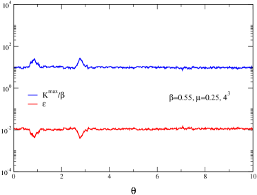
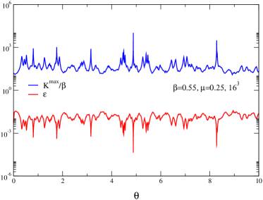
Figure 2: Example of the Langevin evolution of the maximal drift term $K^{\rm max}/\beta$ and the adaptive stepsize $\epsilon_{n}$ in the three-dimensional XY model with $\beta=0.55$ and $\mu=0.25$ (left) and $\beta=0.1$ and $\mu=2$ (right) on lattices of size $4^{3}$ (top), $10^{3}$ (middle) and $16^{3}$ (bottom). The input stepsize is $\bar{\epsilon}=0.01$. Note the vertical logarithmic scale.

To illustrate the method, we introduce two related models with a real action: the XY model with imaginary chemical potential $\mu=i\mu_{\rm I}$, with the action

$$S_{\rm imag}=-\beta\sum_{x,\nu}\cos\left(\phi_{x}-\phi_{x+\hat{\nu}}+\mu_{\rm I}\delta_{\nu,0}\right),$$ (3.4)

and the phase quenched theory, obtained by taking the absolute value of the complex weight, i.e. $e^{-S}\to|e^{-S}|\equiv e^{-S_{\rm pq}}$, which yields the action

$$S_{\rm pq}=-\beta\sum_{x,\nu}\cos\left(\phi_{x}-\phi_{x+\hat{\nu}}\right)\cosh\left(\mu\delta_{\nu,0}\right).$$ (3.5)

This is the anisotropic XY model, with direction-dependent coupling $\beta_{\nu}$, where $\beta_{0}=\beta\cosh\mu$ and $\beta_{i}=\beta$ ($i=1,2$). Both models are solved using real Langevin dynamics. The drift terms are bounded and there are no instabilities.

In Fig. 3 we show the expectation value of the action density $\langle S\rangle/\Omega$ in the high-$\beta$ phase, at $\beta=0.55$, for small values of $\mu^{2}$. The lattice sizes are $6^{3}$ and $8^{3}$, showing that finite size effects are under control. The result at imaginary $\mu$ appears at $\mu^{2}<0$, while the full and phase quenched results are plotted at $\mu^{2}>0$. At $\mu=0$ all results agree (within the statistical error). The full and phase quenched results differ, as can be expected from e.g. a Taylor expansion of the observable for small $\mu$. The results for imaginary and real $\mu$ appear continuous around $\mu^{2}=0$, which is expected from the analyticity of the partition function in $\mu^{2}$ on a finite lattice. The lines indicate second-order fits to the data on the $6^{3}$ lattice, with the results

$$\langle S\rangle/\Omega= -0.9433(7)-0.502(4)\mu^{2}+0.19(1)\mu^{4},$$ (3.6)

$$\langle S\rangle_{\rm pq}/\Omega= -0.940(2)\,\,\,-0.35(2)\mu^{2}\,\,\,-0.04(3)\mu^{4}.$$ (3.7)

In the first case, the data at real and imaginary $\mu$ are combined in the fit.

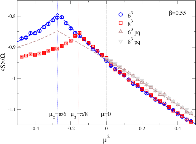
Figure 3: Action density $\langle S\rangle/\Omega$ in the three-dimensional XY model as a function of $\mu^{2}$ at $\beta=0.55$ on lattices of size $6^{3}$ and $8^{3}$, for the full theory (circle, square, $\mu^{2}>0$), at imaginary $\mu$ (circle, square, $\mu^{2}<0$), and phase quenched (triangles, $\mu^{2}>0$). The vertical lines at $\mu_{\rm I}=\pi/N_{\tau}$ indicate the Roberge-Weiss lines at imaginary $\mu$. The dashed lines are the second-order fits (3.6, 3.7), incorporating the RW reflection symmetry.

For imaginary $\mu$ we observe a cusp at $\mu_{\rm I}=\pi/N_{\tau}$. This is similar to the Roberge-Weiss transition in QCD [21, 22] and is due to the periodicity $\mu_{\rm I}\to\mu_{\rm I}+2\pi/N_{\tau}$. Note that the dashed lines in Fig. 3 reflect this symmetry. It would therefore be interesting to determine the phase structure of the XY model at imaginary chemical potential and finite $N_{\tau}$. In the three-dimensional thermodynamic limit ($N_{\tau}$ is taken to infinity as well) and vanishing chemical potential, the magnetized and symmetric phase are separated at the critical coupling $\beta_{c}(\mu=0)$. Consequently it is intriguing to analyse the interplay between the putative Roberge-Weiss transition and the standard magnetization transition in this limit, in particular since it would result in a breakdown of analyticity of $\beta_{c}(\mu^{2})$ around $\mu^{2}=0$ and make $\beta_{c}(\mu=0)$ a multicritical point.

4 Heavy dense limit of QCD

To show the generality of the adaptive stepsize method we now apply it to the heavy dense limit of QCD in four dimensions. Here we shall present results obtained with the second algorithm. The stochastic quantization for this theory was studied in Ref. [6]. Here we briefly repeat the essential equations; we refer to Ref. [6] for further details.

The gluonic part of the action is the standard Wilson SU(3) action,

$$S_{B}[U]=-\beta\sum_{x}\mathop{\sum_{\mu,\nu}}_{\mu<\nu}\left(\frac{1}{6}\left[\mbox{Tr}\,U_{x,\mu\nu}+\mbox{Tr}\,U_{x,\mu\nu}^{-1}\right]-1\right),$$ (4.1)

where $U_{x,\mu\nu}$ are the plaquettes and $\beta=6/g^{2}$. The fermion determinant (starting from Wilson fermions) is approximated as

$$\det M\approx\prod_{{\mathbf{x}}}\det\left(1+he^{\mu/T}{\cal P}_{{\mathbf{x}}}\right)^{2}\det\left(1+he^{-\mu/T}{\cal P}_{{\mathbf{x}}}^{-1}\right)^{2},$$ (4.2)

where $h=(2\kappa)^{N_{\tau}}$. Here $\kappa$ is the Wilson hopping parameter and $N_{\tau}=1/T$ the number of sites in the temporal direction. The lattice spacing $a\equiv 1$. The determinant refers to colour space only. The (conjugate) Polyakov loops are

$${\cal P}_{\mathbf{x}}=\prod_{\tau=0}^{N_{\tau}-1}U_{(\tau,{\mathbf{x}}),4},\;\;\;\;\;\;\;\;\;\;\;\;\;\;\;\;{\cal P}_{\mathbf{x}}^{-1}=\prod_{\tau=N_{\tau}-1}^{0}U_{(\tau,{\mathbf{x}}),4}^{-1}.$$ (4.3)

A formal derivation of Eq. (4.2) follows by considering the heavy ($\kappa\to 0$) and dense ($\mu\to\infty$) limit, keeping the product $\kappa e^{\mu}$ fixed (see Ref. [23] and references therein). The anti-quark contribution is kept to preserve the symmetry under complex conjugation.

The Langevin process is

$$U_{x,\mu}^{\prime}=R_{x,\mu}\,U_{x,\mu},\;\;\;\;\;\;\;\;\;\;\;\;R_{x,\mu}=\exp\left[i\lambda_{a}\left(\epsilon K_{x\mu a}+\sqrt{\epsilon}\eta_{x\mu a}\right)\right],$$ (4.4)

where $\lambda_{a}$ are the Gell-Mann matrices and the noise satisfies $\langle\eta_{x\mu a}\rangle=0$, $\langle\eta_{x\mu a}\eta_{y\nu b}\rangle=2\delta_{\mu\nu}\delta_{ab}\delta_{xy}$. The drift term $K_{x\mu a}=-D_{x\mu a}\left(S_{B}+S_{F}\right)$, where $S_{F}=-\ln\det M$, is complex due to the fermion contribution. For explicit expressions, see Ref. [6].

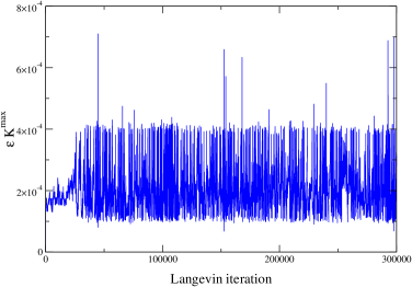
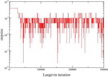
Figure 4: Example of the Langevin evolution of the maximal drift term $\epsilon K^{\rm max}$ (left) and the adaptive stepsize $\epsilon$ (right) in the heavy dense limit of QCD with $\beta=5$, $\kappa=0.12$ and $\mu=0.7$ on a lattice of size $2^{4}$, using ${\cal K}=2\times 10^{-4}$.

Figure 5: As above for $\frac{1}{3}\mbox{Tr}\,U_{4}U_{4}^{{\dagger}}$, indicating the deviation from unitarity during the evolution.

This Langevin process suffers from instabilities, which can be partially controlled using small enough stepsize. Applying the second formulation of the adaptive stepsize algorithm completely eliminates runaways. In this setup measurements are performed after a Langevin time interval of length $\Delta\vartheta$ (this defines one “iteration”). The number of sweeps $N_{\rm sweep}$ in an iteration depends on the Langevin timestep $\epsilon$: if the latter is decreased by a factor $p$, $N_{\rm sweep}$ is increased by the same factor, and conversely. This makes the statistical analysis straightforward, since each iteration has the same weight $\Delta\vartheta=\epsilon\,N_{\rm sweep}$. Note that $N_{\rm sweep}$ will no longer be decreased and correspondingly $\epsilon$ will no longer be increased if the former reaches 1.

To demonstrate this approach, we show in Fig. 4 a characteristic evolution of $\epsilon K^{\rm max}$ (left) and the stepsize $\epsilon$ (right), using ${\cal K}=2\times 10^{-4}$ and $p=2$, with initial $\epsilon=1\times 10^{-5}$, $N_{\rm sweep}=16$. The total number of iterations is $N_{\rm iter}=3\times 10^{5}$ leading to a total Langevin time $\vartheta_{\rm tot}=N_{\rm iter}\times\Delta\vartheta=48$. Varying these input parameters by factors of two or more does not change the results but may only affect the statistics. $K^{\rm max}$ is the maximum value of $|K_{x\mu a}|$ over $x$, $\mu$ and $a$ in the last sweep of an iteration. We observe that the product $\epsilon K^{\rm max}$ remains bounded, as required, while the stepsize (and hence $K^{\rm max}$) fluctuate substantially. In Fig. 5 we show the evolution of $\frac{1}{3}\mbox{Tr}\,U_{4}U_{4}^{{\dagger}}$, which measures the deviation from unitarity [6], acknowledging the typical fluctuations in stationary regime.

As mentioned above, after the implementation of this algorithm, we have not encountered any instability.

5 Conclusion

Instabilities can make complex Langevin simulations extremely problematic. We have shown that they result from large fluctuations in the magnitude of the drift term and the presence of unstable directions in complexified field space. This can be cured by using an adaptive time-local stepsize. The scheme is generic and could be applied to other theories such as QCD. While we have no proof that stable evolution is guaranteed, we have not encountered any instability using this method in the XY model at finite chemical potential and QCD in the heavy dense limit, for a wide selection of parameter values and system sizes. With a fixed stepsize on the other hand, instabilities can be so frequent that it is virtually impossible to generate a thermalized ensemble.

Runaways are due to specific instabilities of the complexified Langevin equations caused by the strong increase of the drift in the non-compact imaginary directions. We have shown that these runaways can be eliminated by using a dynamical step size, which indicates that they are not a question of principle for complex Langevin dynamics but one of numerical accuracy in following the trajectories. We consider this to be an important result of our analysis. Of course, for practical calculations one should consider further optimization of the algorithms by applying methods developed for general real Langevin processes (see, e.g., Ref. [24]) after analysing their adequacy to the complex Langevin problems of interest.

We emphasize that the adaptive stepsize permits a fine tracing of the drift trajectories. If the process picks up a diverging trajectory the noise term will typically kick the process off it. The present results suggest therefore that runaways are not due to following diverging trajectories [25] but rather due to following “wrong” trajectories, i.e. trajectories which, because of accumulating errors in the evaluation of the drift, do not belong to the dynamics of the problem. This both stresses the necessity of ensuring precision in the calculation and helps in disentangling various sources of deficiency in the search for a reliable method.

Acknowledgments.

We thank Simon Hands, Owe Philipsen and Denes Sexty for discussions. I.-O.S. thanks the MPI for Physics München and Swansea University for hospitality. G.A. and F.J. thank the Blue C Facility at Swansea University for computational resources. G.A. and F.J. are supported by STFC.

References

- [1] G. Parisi and Y. s. Wu, Sci. Sin. 24 (1981) 483.
- [2] G. Parisi, Phys. Lett. B 131 (1983) 393.
- [3] J. R. Klauder, Stochastic quantization, in: H. Mitter, C.B. Lang (Eds.), Recent Developments in High-Energy Physics, Springer-Verlag, Wien, 1983, p. 351.
- [4] P. H. Damgaard and H. Hüffel, Phys. Rept. 152 (1987) 227.
- [5] F. Karsch and H. W. Wyld, Phys. Rev. Lett. 55 (1985) 2242.
- [6] G. Aarts and I.-O. Stamatescu, JHEP 0809 (2008) 018 [0807.1597 [hep-lat]].
- [7] G. Aarts, Phys. Rev. Lett. 102 (2009) 131601 [0810.2089 [hep-lat]].
- [8] G. Aarts, JHEP 0905 (2009) 052 [0902.4686 [hep-lat]].
- [9] J. Berges and I.-O. Stamatescu, Phys. Rev. Lett. 95 (2005) 202003 [hep-lat/0508030].
- [10] J. Berges, S. Borsanyi, D. Sexty and I. O. Stamatescu, Phys. Rev. D 75 (2007) 045007 [hep-lat/0609058].
- [11] J. Berges and D. Sexty, Nucl. Phys. B 799 (2008) 306 [0708.0779 [hep-lat]].
- [12] C. W. Bernard and V. M. Savage, Phys. Rev. D 64 (2001) 085010 [hep-lat/0106009].
- [13] C. Pehlevan and G. Guralnik, Nucl. Phys. B 811, 519 (2009) [0710.3756 [hep-th]], Nucl. Phys. B 822 (2009) 349 [0902.1503 [hep-lat]].
- [14] J. R. Klauder and W. P. Petersen, J. Stat. Phys. 39 (1985) 53.
- [15] J. Ambjorn and S. K. Yang, Phys. Lett. B 165 (1985) 140.
- [16] J. Ambjorn, M. Flensburg and C. Peterson, Nucl. Phys. B 275 (1986) 375.
- [17] S. Chandrasekharan, PoS LATTICE2008 (2008) 003 [0810.2419 [hep-lat]].
- [18] P. Hasenfratz and F. Karsch, Phys. Lett. B 125 (1983) 308.
- [19] M. G. Endres, Phys. Rev. D 75 (2007) 065012 [hep-lat/0610029].
- [20] M. Campostrini, M. Hasenbusch, A. Pelissetto, P. Rossi and E. Vicari, Phys. Rev. B 63 (2001) 214503 [cond-mat/0010360].
- [21] A. Roberge and N. Weiss, Nucl. Phys. B 275, 734 (1986).
- [22] P. de Forcrand and O. Philipsen, Nucl. Phys. B 642 (2002) 290 [hep-lat/0205016].
- [23] R. De Pietri, A. Feo, E. Seiler and I. O. Stamatescu, Phys. Rev. D 76 (2007) 114501 [0705.3420 [hep-lat]].
- [24] W. P. Petersen, hep-lat/9602008.
- [25] G. Aarts, E. Seiler and I. O. Stamatescu, Phys. Rev. D (to appear) [0912.3360 [hep-lat]].