Isometric Multi-Manifolds Learning

Abstract

Isometric feature mapping (Isomap) is a promising manifold learning method. However, Isomap fails to work on data which distribute on clusters in a single manifold or manifolds. Many works have been done on extending Isomap to multi-manifolds learning. In this paper, we proposed a new multi-manifolds learning algorithm (M-Isomap) with the help of a general procedure. The new algorithm preserves intra-manifold geodesics and multiple inter-manifolds edges faithfully. Compared with previous approaches, this algorithm can isometrically learn data distribute on several manifolds. Some revisions have been made on the original multi-cluster manifold learning algorithm called D-C Isomap [24] such that the revised D-C Isomap can learn multi-manifolds data. Finally, the features and effectiveness of the proposed multi-manifolds learning algorithms are demonstrated and compared through experiments.

I Introduction

Challenges, known as ”the curse of dimensionality”, are usually confronted when scientists are doing researches on high dimensional data. Dimensionality reduction is a promising tool to circumvent these problems. Principal component analysis (PCA) [1] and multidimensional scaling (MDS) [2] are two important linear dimensionality reduction methods. Due to their linear model assumption, both of the methods will fail to discover nonlinear intrinsic structure of data.

Recently, there are more and more interests in nonlinear dimensionality reduction (NLDR). NLDR is used to learn nonlinear intrinsic structure of data, which is considered to be the first step of ”machine learning and pattern recognition: observe and explore the phenomena”[3]. Two interesting nonlinear dimensionality reduction methods based on the notion of manifold learning[6], isometric feature mapping (Isomap)[4] and local linear embedding (LLE)[5], have been introduced in SCIENCE 2000. LLE assumes that data points locally distribute on a linear patch of a manifold. It preserves local linear coefficients, which best reconstruct each data point by its neighbors, into a lower dimensional space. Isomap is based on classical MDS method. Instead of preserving pairwise Euclidean distance, it preserves geodesic distance on the manifold. The geodesic between two data points is approximated by the shortest path on a constructed graph. Both of the methods are computational efficient and able to achieves global optimality. Besides, there are many other important nonlinear dimensionality reduction methods. Laplacian eigenmap[7] utilizes the approximation of the Laplace-Beltrami operator on manifold to provide an optimal embedding. Hessian LLE[8] resembles Laplacian eigenmap by using the approximation of Hessian operator instead of Laplacian operator. Local tangent space alignment(LTSA)[9] method learns local geometry by constructing a local tangent space of each data point and then aligns these local tangent spaces into a single global coordinates system with respect to the underlying manifold. Diffusion maps[10] applies diffusion semigroups to produce multiscale geometries to represent complex structure. Riemannian manifold learning (RML)[11] method uses the constructed Riemannian normal coordinate chart to map the input data into a lower dimensional space. NLDR is fast developed and has been proved very useful in many fields and applications, such as classification using Isomap[16] and laplacian eigenmap[17], geometric based semi-supervised learning method using laplacian eigenmap[18], data visualization [19], time series manifold learning[20, 21] and so on.

As Isomap emphasizes on the global geometric relationship of data points, it is very illustrative in data visualization and pattern analysis[13]. Although Isomap algorithm implicitly requires the data set is convex, it still demonstrates very meaningful results on non convex data sets. Therefore, in this paper, we will focus attention on extending Isomap to multi-manifolds learning. The first step of Isomap algorithm is to construct a neighborhood graph which connects all the data points. This step is of vital importance because the success of following steps depend on how well the constructed neighborhood graph is. However, it is hard to build a totally connected neighborhood graph and guarantee the topological stability of classical Isomap algorithm when points of the data set distribute on clusters in a manifold or manifolds (multiple manifolds). Many works have been done on extending Isomap to multi-manifolds data. Some methods try to do this by providing new neighborhood graph construction algorithms. Yiming Wu et al [23] introduced a split and augment procedure for neighborhood graph construction which could produce a totally connected neighborhood graph. Li Yang [28, 26, 29, 27] introduced several neighborhood graph construction algorithms using techniques from discrete mathematics, graph theory. Deyu Meng et al[24] proposed a decomposition and composition Isomap (D-C Isomap).

The rest of the paper is organized as follows: In Section II, main issues and limitations of classical Isomap algorithm are presented. The problem of multi-manifolds learning is also investigated. In Section III, previous methods on multi-manifolds learning are briefly introduced and discussed. In Section IV, a general procedure for designing multi-manifolds learning algorithms is first proposed. With the proposed procedure, a new multi-manifolds learning algorithm (M-Isomap) is designed and analyzed. With some revisions on the original algorithm, the main limitations of D-C Isomap are resolved. Finally, in Section V, the effectiveness of these multi-manifolds learning algorithms has been demonstrated by experiments. Comparisons of these algorithms have also been made.

II Classical Isometric Feature Mapping and Its Limitations

Isomap is able to recover the intrinsic geometric structure and converge as the number of data points increases[4] if data lie on a manifold, . Like PCA and MDS, Isomap has the advantage of simple implementation and computational efficiency. The algorithm also guarantees a globally optimal solution.

It is assumed that data set $X=\{x_{1},x_{2},\cdots,x_{N}\}$ is in high dimensional space $R^{D}$ and the feature space is $R^{d}$. The classical Isomap algorithm has three steps.

1. Step 1: Identify the neighbors for all the data points to construct a neighborhood graph. With the given parameter $k$ or $\epsilon$, there are two ways to construct a neighborhood graph for $X$:

   • if $x_{j}$ is one of $x_{i}$’s k nearest neighbors, they are connected by an edge (the k-NN method).

   • $x_{i}$ and $x_{j}$ satisfy $\|x_{i}-x_{j}\|<\varepsilon$, they are connected by an edge (the $\varepsilon$-NN method).

2. Step 2: Use Dijkstra’s or Floyd-Warshall algorithm to compute the length of shortest path $d_{G}(x_{i},x_{j})$ between any couple of data points $x_{i}$ and $x_{j}$ on the graph. It is proved that $d_{G}(x_{i},x_{j})$ is a good approximation of geodesic distance $d_{M}(x_{i},x_{j})$ on the manifold as the number of data points increases.

3. Step 3: Perform classical MDS on the graph distance matrix $D_{G}$ whose $(i,j)$-th element is $d_{G}(i,j)$. Minimize a cost function

   $${{E(Y)=\|\tau(D_{G})-\tau(D_{Y})\|_{F_{2}}}}$$

   The operator $\tau$ is defined as $\tau(D)=-\frac{HSH}{2}$, where $H=I-\frac{1}{n}ee^{T}$, $S=(D_{i,j}^{2})$, $I$ is the identity matrix and $e=(1,1,\cdots,1)^{T}$. $D_{Y}=(\|y_{i}-y_{j}\|)$. Assuming that, in decreasing order, $\lambda_{i}$ is the $i$-th eigenvalue of $\tau(D_{G})$ and $\nu_{i}$ is the corresponding eigenvector to $\lambda_{i}$, then the low dimensional embedding $Y$ is given by:

   $$Y=[y_{1},,y_{2},\cdots,y_{n}]=\begin{pmatrix}\sqrt{\lambda_{1}}\nu_{1}^{T}\\ \cdots\\ \sqrt{\lambda_{d}}\nu_{d}^{T}\end{pmatrix}$$

The properties of Isomap algorithm are well understood [14][12]. However, the success of Isomap algorithm depends on two issues. One issue is how to choose the correct intrinsic dimensionality $d$. Setting a lower dimensionality $d$ will lead to a loss of data structure information. On the other hand, setting a higher dimensionality $d$ will cause that redundant information is kept. This issue has been well investigated. The other issue is the quality of the constructed neighborhood graph. It is known that the problem on neighborhood graph construction is still a tricky one. Both the k-NN and $\varepsilon$-NN methods have their limitations. Under the assumption that data points distribute on a single manifold, if the neighborhood size $k$ or $\varepsilon$ is chosen too small, the constructed neighborhood graph will be very sparse. Thus geodesics can not be satisfyingly approximated. Otherwise, if neighborhood size $k$ or $\epsilon$ is chosen too large to cause short-circuit edges, these edges will have a significant negative influence on the topological stability of Isomap algorithm[22].

Nonetheless, it is a relative simpler problem if data points distribute uniformly on one manifold. Both the ”short circuit” and ”discontinuity” problem can be circumvented by carefully choosing an appropriate neighborhood size $k$ or $\varepsilon$. It is a different problem if the data distribute on clusters or manifolds. k-NN or $\varepsilon$-NN do not guarantee that the whole data set is totally connected and the quality of approximated geodesics.

In real world, ”data missing” and ”data mixture” are common problems in data analysis. Under manifold assumption, these two problems cause that data distribute on different clusters in a manifold or manifolds. Here, the main problems of multi-manifolds learning are presented, the data may have these properties: First, data points on different manifolds may have different input dimensionality $D$ (dimensionality of the ambient space). This usually happens in ”data mixture” cases. Second, learning different data manifolds may need different value of input parameters, i.e. appropriate neighborhood size ($k$ or $\varepsilon$) and intrinsic dimensionality $d$ for each data manifold. The case when data points distribute on pieces of a single manifold is referred to as multi-cluster manifold learning; meanwhile, the case when data points distribute on multiple manifolds is referred to as multi-manifolds learning. In this paper, we will concentrate on designing multi-manifolds learning algorithms to data with these properties.

III Previous Works on Multi-Manifolds Learning

III-A Multi-manifolds learning by new neighborhood graph construction method

Wu and Chan [23] proposed a split-augment approach to construct a neighborhood graph. Their method can be regarded as a variation of the k-NN method and can be summarized as below:

1. k-NN method is applied to the data set. Every data point is connected with its neighbors. If the data lies on multiple manifolds, several disconnected graph components (data manifolds) will be formed.

2. Each couple of graph components are connected by their nearest couple of inter-components points.

This method is simple to implement and has the same computational complexity as k-NN method. However, as there is only one edge connecting every two graph components, geodesics across components are poorly approximated; meanwhile, their low dimensional embedding can be rotated arbitrarily. This method can not be directly applied to data lying on three or more data manifolds. If more than two graph components exist, intra-component shortest distances may be changed in the totally connected graph.

Li [26, 27, 28, 29] introduced four methods to construct a connected neighborhood graph. The k minimum spanning trees (k-MST)[26] method repeatly extracts k minimum spanning trees (MSTs) from the complete Euclidean graph of all data points. Edges of the k MSTs form a k-connected neighborhood graph. Instead of extracting k MSTs, the minimum-k-spanning trees (min-k-ST)[27] method finds k edge-disjoint spanning trees from the complete Euclidean graph, and the sum of the total edge length of the k edge-disjoint spanning trees attains a minimum. The k-edge-connected (k-EC)[28] method constructs a connected neighborhood graph by adding edges in a non-increasing order from the complete Euclidean graph. An edge is added if its two end vertices do not have k edge-disjoint paths connected with each other. The k-vertices-connected (k-VC)[29] method add edges in a non-increasing order from the complete Euclidean graph, an edge is added if its two end vertices would be disconnected by removing some $k-1$ vertices. Finally, the constructed neighborhood graph would not be disconnected by removing any $k-1$ vertices.

The methods introduced in [26, 27, 28, 29] advantage over k-NN method for two reasons: First, the local neighbor relationship is affected by the global distribution of data points. This is beneficial for adaptively preservation of the global geometric metrics. Second, these methods could guarantee that the constructed neighborhood graph is totally connected. Compared with k-NN method, Li’s methods construct a neighborhood graph with more edges corresponding to the same neighborhood size $k$. This property can assure the quality of the neighborhood graphs.

III-B Multi-manifolds learning by decomposition-composition Isomap

In [24], Meng et al. proposed a decomposition-composition method (D-C Isomap) which extends Isomap to multi-cluster manifold learning. The purpose of their method is to preserve intra-cluster and inter-cluster distances separately. Because a revised version of D-C Isomap will be introduced in the next section, we present the details of D-C Isomap algorithm in the following

Step I: decomposition process

1. Given neighborhood size $k$ or $\varepsilon$, if the data is of multi-cluster, several disconnected graph components can be identified when every data point is connected with its neighbors by k-NN or $\varepsilon$-NN.

2. Assuming that there are $M$ components, the $m$-th component is also denoted as a cluster $X^{m}=\{x_{1}^{m},\cdots,x_{l_{m}}^{m}\}$. Clusters $X^{m}$ and $X^{n}$ are connected by their nearest inter-cluster data points $nx^{m}_{n}$ and $nx^{n}_{m}$ whose pairwise distance is assumed to be $d^{0}_{m,n}$.

3. Apply k-NN Isomap or $\epsilon$-NN Isomap on each cluster $X^{m}$. Denote the geodesic distance matrix for $X^{m}$ as $D^{m}=(D^{m}_{i,j})$, the corresponding low dimensional embedding as $Y^{m}=\{y^{m}_{1},\cdots,y^{m}_{l_{m}}\}$, and the embedding point corresponding to $nx^{m}_{n}$ as $ny^{m}_{n}$, where $ny^{m}_{n}\in Y^{m}$ .

Step II: composition process

1. The set of centers of clusters is denoted as $CX=\{cx_{1},\cdots,cx_{M}\}$, where every center is computed by

   $$cx_{m}=\underset{x_{i}\in X^{m}}{\arg\min}\left(\underset{x_{j}\in X^{m}}{\max}(D_{ij}^{m})\right)\qquad m=1,\cdots,M.$$

2. The distance matrix for $CX$ can be computed by

   $$\tilde{D}=\{\tilde{D}_{mn}\},\qquad\tilde{D}_{mn}=\left\{\begin{array}[]{ll}d_{m,n}+d_{m,n}^{0}+d_{n,m}&m\not=n\\ 0,&m=n\end{array}\right.$$

   
   

   where $d_{m,n}$ is the distance of shortest path between $cx_{m}$ and $nx_{n}^{m}$ on the graph component $X^{m}$.

3. Plug distance matrix $\tilde{D}$ and neighborhood size $d$ into classical Isomap algorithm. The embedding of $CX$ is denoted by $CY=\{cy_{1},\cdots,cy_{M}\}\subset\mathbb{R}^{d}$ ($CY$ is called the translation reference set). Assuming that the $d$ nearest neighbors of $cx_{m}$ are $\{cx_{m_{1}},\cdots,cx_{m_{d}}\}$, the low dimensional representation corresponding to $nx_{m_{i}}^{m}$ is computed as

   $$sy_{m_{i}}^{m}=cy_{m}+\frac{d_{m,m_{i}}}{d_{m,m_{i}}+d_{m,m_{i}}^{0}+d_{m_{i},m}}(cy_{m_{i}}-cy_{m})$$

   $i=1,\cdots,d,\quad m=1,\cdots,M.$

4. Construct the rotation matrix $\mathcal{A}_{m}$ for $Y^{m},m=1,\cdots,M.$ Assuming that $QN_{m}$ is the principal component matrix of $NY_{m}=\{ny_{m1}^{m},\cdots,ny_{m_{d}}^{m}\}$ and $QS_{m}$ is the principal component matrix of $SY_{m}=\{sy_{m1}^{m},\cdots,sy_{m_{d}}^{m}\}$, then the rotation matrix for $Y^{m}$ is $\mathcal{A}_{m}=QS_{m}QN_{m}^{T}$.

5. Transform $Y^{m},m=1,\cdots,M$ into a single coordinate system by Euclidean transformations

   $$FY^{m}=\{fy_{i}^{m}=\mathcal{A}_{m}y_{i}^{m}+cy_{m},i=1,\cdots,l_{m}\},\quad m=1,\cdots,M.$$

Then $Y=\bigcup_{m=1}^{M}FY^{m}$ is the final output.

Firstly, the D-C Isomap reduces the dimensionality of clusters separately; meanwhile, it preserves a skeleton of the whole data. Secondly, using Euclidean transformations, embedding of each cluster is placed into the corresponding position by referring to the skeleton. In this way, intra-cluster geodesics are exactly preserved. As D-C Isomap method uses circumcenters to construct the skeleton of whole data, its learning results unstably depend on the mutual position of these circumcenters. It is known that at least $d+1$ reference points are needed to anchor a $d$-dimensional simplex. However, in D-C Isomap algorithm, the number of the reference data points is limited by the number of clusters.

III-C Constrained Maximum Variance Mapping

There is also a newly proposed algorithm called constrained maximum variance mapping (CMVM)[25] for multi-manifolds learning. CMVM method is proposed on the notion of maximizing dissimilarities between classes while holding up the intra-class similarity.

IV Isometric Multi-Manifolds Learning

TABLE I: Symbols and Variables used in the Algorithms

$X=\{x_{i}\}_{i=1}^{N}$	The total data set, with $x_{i}\in{\mathbb{R}}^{D}$
$X^{m}=\{x_{i}^{m}\}_{i=1}^{S_{m}}$	The m-th data manifold, where $m=1,\cdots,M$
$Y^{m}=\{y_{i}^{m}\}_{i=1}^{S_{m}}$	Low dimensional embedding of $X^{m}$
$D_{mn}=(d_{I}(i,j))$	Matrix of geodesic distances across data manifolds $X^{m}$ and $X^{n}$
$fx_{n}^{m}$, $fx_{m}^{n}$	The furthest couple of data points between $X^{m}$ and $X^{n}$
$\{x_{n(i)}^{m}\}_{i=1}^{k}$	Subset of $X^{m}$, data points of which are the nearest ones to $X^{n}$
$I^{m}=\{x_{i}^{m}\}_{i=1}^{l_{m}}$	The selected data points from $X^{m}$ to construct the skeleton $I$
$I=\bigcup_{m=1}^{M}I^{m}$	Points which are used to construct a skeleton $I$ of $X$
$D_{I}$	Approximated geodesic distance matrix for skeleton $I$
$RY_{I}$	Low dimensional embedding of the skeleton $I$
$RY_{I}^{m}\subset RY_{I}$	Low dimensional embedding of $I^{m}$, which will also be referred
	as the transform reference for $Y^{m}$
$nx_{j}^{i}$	The point in $X^{i}$ which is the nearest to $X^{j}$, or the inter-cluster point
	in D-C Isomap algorithm.

IV-A The general procedure for isometric multi-manifolds learning

Many previous methods extend Isomap for multi-manifolds learning by revising the neighborhood graph construction step of the Isomap algorithm[23, 28, 26, 29, 27]. However, shortest paths across clusters or data manifolds are bad approximations of geodesics. In Isomap, bad local approximation always leads to the deformation of global low dimensional embedding.

Under the continuous assumption, it is assumed that $\Omega$ is an open, convex and compact set in ${\mathbb{R}}^{d}$, and $f:\Omega\to{\mathbb{R}}^{D},d<<D$ is a continues mapping. $f(\Omega)=\mathcal{M}$ is defined as a $d$ dimensional parameterized manifold. $K(x,y)$ $(x,y\in\mathcal{M})$ is a specially defined kernel and a reproducing kernel Hilbert space (RKHS) $\mathscr{H}$ is constructed with this kernel. $\phiup_{j}(x)$ is the eigenfunction corresponding to the $j$-th largest eigenvalue $\lambda_{j}$ of $K(x,y)$ in $\mathscr{H}$, which is also the $j$-th element of Isomap embedding. The geodesic distance on manifold $\mathcal{M}$ is written as $d^{2}(x,y)=d^{2}(f(\tau),f(\overset{\wedge}{\tau}))=\alpha\|\tau-\overset{\wedge}{\tau}\|+\eta(\tau,\overset{\wedge}{\tau}),$ where $\tau,\overset{\wedge}{\tau}\in\Omega$, $\alpha$ is a constant and $\eta(\tau,\overset{\wedge}{\tau})$ is the deviation from isometry. The constant vector

$$C=\frac{\int_{\mathcal{M}}x\rhoup(x)dx}{\int_{\mathcal{M}}\rhoup(x)dx}=\frac{\int_{\Omega}\tau\mathcal{H}(\tau)d\tau}{\int_{\Omega}\mathcal{H}(\tau)d\tau}$$

where $\rhoup(x)$ and $\mathcal{H}(\tau)$ are density functions of $\mathcal{M}$ and $\Omega$. With the assumptions above, the following theorem is proved by Zha et al [12].

Theorem IV.1

There is a constant vector $P_{j}$ such that $\phiup_{j}(x)=P_{j}^{T}(\tau-C)+e_{j}(\tau)$, where $e_{j}(\tau)=\epsilon_{j}^{(0)}-\epsilon_{j}(\tau)$ has zero mean, i.e., $\int_{\Omega}\mathcal{H}(\tau)e_{j}(\tau)d\tau=0$, with $\epsilon_{j}(\tau)=\frac{1}{2\lambda_{j}}\int_{\Omega}\eta(\tau,\overset{\wedge}{\tau})\mathcal{H}(\overset{\wedge}{\tau})\phiup_{j}(x)d\overset{\wedge}{\tau}$, $\epsilon_{j}^{(0)}=\frac{1}{\int_{\Omega}\mathcal{H}(\tau)d\tau}\int_{\Omega}\epsilon_{j}(\tau)\mathcal{H}(\tau)d\tau$.

By theorem 4.1, even if the deviation $\eta(\tau,\overset{\wedge}{\tau})$ is not zero with only a limited range of $(\tau,\overset{\wedge}{\tau})$. The coordinate of the low dimensional embedding $\phiup_{j}(x)$ is still deformed, and the deformation is measured by $e_{j}(\tau)$.

In order to get a better understanding of multi-manifolds data, it is profitable to preserve intra-manifold relationship (where $\eta(\tau,\overset{\wedge}{\tau})=0$) and inter-manifolds relationship (where $\eta(\tau,\overset{\wedge}{\tau})\not=0$) separately. This is because that sometimes we care more about the information within the same data manifold. Here we propose a general procedure for isometric multi-manifolds learning algorithms.

Step I: The decomposition process

1. Cluster the whole data set. If data distribute on different clusters in a manifold or manifolds, the clusters or manifolds should be identified. Many clustering method could be used, such as K-means, Isodata and methods introduced in [15][33]. Even if the manifolds overlay with each other, they can still be identified and clustered[39]. At this step, data set $X$ is clustered into several components and every component is considered as a data manifold.

2. Estimate parameters of data manifolds. For intrinsic dimensionality estimation, many methods can be used: the fractal based method [34], MLE method [35, 36], and the incising ball method [37]. Assume that $d_{m}$ is the intrinsic dimensionality of the $m$-th data manifold. Let $d=\underset{m}{\max{d_{m}}}$. For neighborhood size, [32] introduces a method on automatically generating parameters for Isomap on one single data manifold. For convenience, appropriate neighborhood sizes ($k_{m}$ or $\varepsilon_{m}$ for $X^{m}$) could be given manually for data manifolds.

3. Learn the data manifolds individually. One data manifold can be learned by traditional manifold learning algorithms. Here, we propose to rebuild a graph on each data manifold with new neighborhood size to better approximate intra-manifold geodesics. Methods of Li’s works [26, 27, 28, 29] or the $k$-CC method is preferred, where the k-CC graph construction method will be described later. It is assumed that the low dimensional embedding for $X^{m}$ is $Y^{m}$.

Step II: The composition process

1. Preserve a skeleton $I$ of the whole data set in low dimensional space ${\mathbb{R}}^{d}$. The skeleton $I$ should be carefully designed such that it can represent the global structure of $X$. Let $RY_{I}$ be the low dimensional embedding of $I$.

2. Transform $Y^{m}$s into a single coordinate system by referring to $I$. In order to faithfully preserve intra-manifold relationship, Euclidean transformations could be constructed and used. Using embedding points $RY^{m}\subset RY^{I}$ and corresponding points from $Y^{m}$, we can construct an Euclidean transformation from $Y^{m}$ to the coordinate system of $I$.

Although the idea about decomposition-composition is not new, which is first used by Wu et al. [23] in their split-augment process and well developed and used in [24]. The procedure we proposed here aims to solve a more general problem. Step I.1 permits that the designed learning method has a good ability to identify data manifolds. Step I.2 gives a guideline on learning manifolds with different intrinsic dimensionality and neighborhood sizes. Step I.3 learns data manifolds individually so that the intra-manifold relationship can be faithfully preserved. Step II.1 is the most flexible part of the procedure which allows us to design new multi-manifolds learning algorithms. A well designed skeleton $I$ could better represent the inter-manifolds relationship. In the following, we will introduce a new multi-manifolds learning algorithm and revise the original D-C Isomap algorithm with the help of this general procedure.

IV-B A new algorithm for isometric multi-manifolds learning

Based on the proposed procedure, we designed a new multi-manifolds learning algorithm. As an extension of Isomap method for multi-manifolds data, the method will be referred to as multi-manifolds Isomap (M-Isomap). It is assumed that $X$ is also interchangeable to represent the matrix $[x_{1},x_{2},\cdots,x_{N}]$, where $\{x_{i},i=1,\cdots,N\}$ are column vectors in ${\mathbb{R}}^{D}$.

IV-B1 Using k-CC method to construct a neighborhood graph and identify manifolds

TABLE II: Computational complexity comparison of k-NN, k-MSTs, Min-k-ST, k-EC and k-VC. TC stands for time complexity and IL stands for the time complexity for incremental learning

	k-NN	k-MST	Ming-k-ST	k-EC	k-VC
TC	$O(kN^{2})$	$O(k^{2}N^{2})$	$O(k^{2}N^{2})$	$O(k^{2}N^{2})$	$O(N^{3})$
IL	O(kN)	$O(N\log N)$			$O(N\log N+kN)$

Table LABEL:tb1 shows the time complexity of k-NN, K-Min-ST, k-EC and k-VC methods on neighborhood graph construction. As it is shown in the table, k-NN method has the lowest computational complexity $O(kN^{2})$.

For incremental learning, the computational complexity of k-NN, k-MSTs and k-VC are $O(kN)$, $O(N\log N)$ and $O(N\log N+kN)$ respectively[30][31]. The computational complexity of Min-k-ST, k-EC methods for incremental learning are unavailable. For data on one single data manifold, the improvement of performance of Li’s methods becomes insignificant when the neighborhood size $k$ for k-NN method increases. More importantly, k-NN implicitly has the property of clustering to multi-manifolds data. Data points of the same manifold tend to be connected by paths and disconnected otherwise when every data point is connected with its neighbors by edges. Although k-NN is not a robust clustering algorithm, it is computational efficient for both clustering and graph construction. Therefore, we introduce a variation of k-NN method which inherits computational advantage of k-NN method. The method is also able to identify data manifolds and construct a totally connected neighborhood graph. In the rest of the paper, the proposed neighborhood graph construction method will be referred as k-edge connected components (the k-CC method).

The summary of k-CC algorithm: First, given a neighborhood size $k$ or $\varepsilon$, every data point is connected with its neighbors. If the data points distribute on several clusters or manifolds, several disconnected graphs will be constructed. Data points are assigned to the same data manifold if there is a path connects them on the graphs. Then, we connect each pair of graphs by $k$ nearest pairs of data points. Concerning about robustness of the algorithm, every data point is only allowed to have one inter-manifolds edge at most.
 

Algorithm:(k-CC method)

Input: Euclidean distance matrix $D$, whose $(i,j)$-th entry is $\|x_{i}-x_{j}\|$. Neighborhood size $k$ or $\varepsilon.$

Output: Graph $G=(V,E)$, number of clusters $M$, label of the data.   
 
Initialization: $V=\{x_{1},\cdots,x_{n}\}$, $V^{\prime}=V$, $E=\phiup$, $Queue=\phi$

0:      for i=1 to $N$ do

0:        Identify nearest neighbors $\{x_{i1},\cdots,x_{il_{i}}\}$ for $x_{i}$ by $k$-nearest-

0:        neighbors or $\varepsilon$-nearest-neighbors. Let $E=E\bigcup\{e_{i1},\cdots e_{il_{i}}\}$

0:      end for

0:      Set $M=1$

0:      while {$V^{\prime}$ is not empty} do

0:         $x\in V^{\prime}$, in-Queue{x}, label(x)=$M$, $V^{\prime}=V^{\prime}-\{x\}$

0:         while {$Queue$ is not empty} do

0:          x=de-Queue

0:           $\forall y$: y is connected with x by an edge

0:           if {y is not labeled} do

0:             in-Queue{y}, label(y)=$M$, $V^{\prime}=V^{\prime}-\{y\}$

0:          end if

0:         end while

0:         $M=M+1$

0:      end while

0:      $M=M-1$

0:   if ( $M\geq$ 2 )

0:     $k=$average($\{l_{i}\}_{i=1}^{N}$)

0:     for $i=1$ to $M$ do

0:        for $j=i+1$ to $M$ do

0:         Find $k$ shortest inter-manifolds edges $e_{1},\cdots,e_{k}$ between

0:          data manifolds $i$ and $j$ and make sure that their ending

0:          vertices are not identical. Let $E=E\bigcup\{e_{1},\cdots,e_{k}\}$

0:        end for

0:      end for

0:   end if

The main difference between k-NN and k-CC is lines (4-25), which identify components (data manifolds) and connect different components of the graph. This change makes the constructed graph totally k-edge connected. Compared with the method proposed in [23], k-CC method constructs a neighborhood graph with $k$ inter-manifolds edges, which is able to control the rotation of the embedding of data manifolds. In Section V, the method, which uses k-CC to construct a totally connected graph and then perform classical Isomap on the graph, will be referred to as k-CC Isomap. It can be easily inferred that k-CC Isomap suffers the limitation which has been shown by Theorem 4.1.

At this step, it is assumed that $X$ is clustered into data manifolds $\{X^{m}\}_{m=1}^{M}$ and $\{x_{n(i)}^{m}\}_{i=1}^{k}$ is the subset of $X^{m}$ whose data points connect with $X^{n(i)},i=1,\cdots,k$.

IV-B2 Learn data manifolds individually

As $X^{m}$ is considered as a single data manifold in $\mathbb{R}^{D}$, it is possible to find its intrinsic parameters. The incising ball method[37] is utilized to estimate the intrinsic dimensionality, which is simple to implement and always outputs an integer result. Assume that $d$ is the highest intrinsic dimensionality of data manifolds. Neighborhood size $k_{m}$ or $\varepsilon_{m}$ of each data manifold is given manually and the graph on data manifold $X^{m}$ is rebuilt. It is hoped that the new neighborhood graph on $X^{m}$ can make better approximations of intra-manifold geodesics. The approximated geodesic distance matrix for $X^{m}$ is written as $D_{m}$. By applying classical MDS on $D_{m}$ , the low dimensional embedding for $X^{m}$ can be got as $Y^{m}=\{y_{i}^{m}\}_{i=1}^{S_{m}}$.

IV-B3 Preserve a skeleton of data manifold $X$

First, inter-manifolds distances are computed. Assuming that $x_{p}^{m}$ and $x_{q}^{n}$ are any data points with $x_{p}^{m}\in X^{m}$ and $x_{q}^{n}\in X^{n}$, their distance can be computed by

$$d(x_{p}^{m},x_{q}^{n})=\underset{t=1\cdots k}{\min}\{d_{m}(x_{p}^{m},x_{n(t)}^{m})+\|x_{n(t)}^{m},x_{m(t^{\prime})}^{n}\|+d_{m}(x_{n(t^{\prime})}^{n},x_{q}^{n})\},$$ (2)

where $d(x_{p}^{m},x_{n(t)}^{m})$ is the shortest path on the neighborhood graph of $X^{m}$. Although $d(x_{p}^{m},x_{n(t)}^{m})$ may not be the shortest path on the totally connected graph of $X$, Eq. (2) is an efficient way to approximate distances across manifolds. $D_{mn}$ is assumed to be the distance matrix across over $X^{m}$ and $X^{n}$. The furthest inter-manifolds data points are computed by

$$\{fx_{n}^{m},fx_{m}^{n}\}=\arg\max d(x_{i}^{m},x_{j}^{n}),\quad d(x_{i}^{m},x_{j}^{n})\in D_{mn}.$$ (3)

Without lose of generality, we assume $I^{m}=\{x_{i}^{m}\}_{i=1}^{l_{m}}=\bigcup_{n=1}^{M}\{x_{n(1)}^{m},\cdots,x_{n(k)}^{m},fx_{n}^{m}\}$ . $I=\bigcup_{m=1}^{M}I^{m}$ is considered as the global skeleton of $X$. On the data manifold $X$, it can be seen that the skeleton $I$ formulates a sparse graph. We assume that $D_{I}=(d_{I}(i,j))$ is the distance matrix of $I$, where

$$d_{I}(i,j)=\left\{\begin{array}[]{ll}d(x_{i}^{m},x_{j}^{n})\in D_{mn},&x_{i}\in X^{m},x_{j}\in X^{n}\\ d(x_{i}^{m},x_{j}^{m})\in D_{m},&x_{i},x_{j}\in X^{m}\end{array}\right.$$ (6)

By applying classical MDS algorithm on $D_{I}$, the low dimensional embedding of $I$ can be got as $RY_{I}$. It is assumed that $RY_{I}^{m}\subset RY_{I}$ is the embedding of $I^{m}$ and $RY_{I}^{m}=\{ry_{i}^{m}\}_{i=1}^{l_{m}}$.

IV-B4 Euclidean transformations

Assuming that $Y_{I}^{m}=\{y_{i}^{m}\}_{i=1}^{l_{m}}\subset Y^{m}$ and $y_{i}^{m}$ corresponds to $x_{i}^{m}$, an Euclidean transformation from $Y^{m}_{I}$ to $RY_{I}^{m}$ could be constructed.

The general Euclidean transformation can be written as

$$ry=\mathcal{A}y+\beta,$$

where $\mathcal{A}$ is an orthonormal matrix and $\beta$ is a position translation vector. For the $m$-th data manifold, it is assumed that the Euclidean transformation is

$$ry_{i}^{m}=\mathcal{A}_{m}y_{i}^{m}+\beta_{m}\quad i=1,\cdots,l_{m},$$

Generally, it could be written in form of matrix

$$RY_{I}^{m} =\mathcal{A}_{m}Y_{I}^{m}+\beta_{m}e^{T} =\begin{pmatrix}\mathcal{A}_{m}&\beta_{m}\end{pmatrix}\begin{pmatrix}Y_{I}^{m}\\ e^{T}\end{pmatrix}$$ (7)

where $e$ is a vector with all ones. Problem (7) can be solved by the least square strategy, and the solution is

$$\begin{pmatrix}\mathcal{A}_{m}&\beta_{m}\end{pmatrix}=RY_{I}^{m}\begin{pmatrix}Y_{I}^{m}\\ e^{T}\end{pmatrix}^{T}\left(\begin{pmatrix}Y_{I}^{m}\\ e^{T}\end{pmatrix}\begin{pmatrix}Y_{I}^{m}\\ e^{T}\end{pmatrix}^{T}+\lambda I\right)^{-1}$$ (8)

where $I$ is the identity matrix and $\lambda$ is the regularization parameter in case singular. However, least square solution does not provides an orthonormal matrix $\mathcal{A}_{m}$. Here we propose to use the orthonormal matrix which is computed by QR decomposition. The QR process can be written as

$$\begin{pmatrix}\mathcal{A}_{m}&R\end{pmatrix}=QR(\mathcal{A}_{m}).$$ (9)

with the diagonal elements of R to be forced non negative. Then $\beta_{m}$ can be recomputed by minimizing a cost function

$$C(\beta_{m}) =\sum_{i=1}^{l_{m}}\|\mathcal{A}_{m}y_{i}^{m}+\beta_{m}-ry_{i}^{m}\|^{2}.$$

By taking derivative $\frac{\partial C(\beta_{m})}{\beta_{m}}=0$, we have

$$\beta_{m}=\frac{1}{l_{m}}\sum_{i=1}^{l_{m}}(ry_{i}^{m}-\mathcal{A}_{m}y_{i}^{m})$$ (10)

Low dimensional embedding $Y_{m},\quad i=1,\cdots,M$ could be translated into a global coordinate system by the constructed Euclidean transformations.

IV-B5 The complete algorithm of M-Isomap

To give an compact presentation of M-Isomap, the algorithm is summarized in the following table.
 
Input: $X=\{{x_{i}}\}_{i=1}^{N}$ with $x_{i}\in\mathbb{R}^{D}$. Initial neighborhood size $k$ or $\varepsilon$. Step I.1 Perform k-CC on $X$. Data manifolds $\{X^{m}\}_{m=1}^{M}$ and the set of inter-manifolds points $\{x_{n(i)}^{m}\}_{i=1}^{k}$ of $X^{m}$ can be obtained. Step I.2 Estimate parameters of data manifolds. It is assumed that intrinsic dimensionality $d_{m}$ and neighborhood size ($k_{m}$ or $\varepsilon_{m}$) are parameters for $X^{m}$. Let $d=\underset{m}{max}\{d_{m}\}$ and rebuild neighborhood graph on $X^{m}$. Step I.3 Classical Isomap is performed on the new graphs superimposed on $X^{m},m=1,\cdots,M$. The corresponding low dimensional embedding of $X^{m}$ is denoted as $Y^{m}$. Step II.1 Inter-manifolds distance matrix $D_{mn}$ is computed by Eq. (2), thus $\{fx_{n}^{m}\}_{m\not=n}^{M}$ can be found by Eq. (3). Distance matrix $D_{I}$ for the skeleton $I$ is computed by Eq. (6). Applying classical MDS on $D_{I}$, we denote the low dimensional embedding of $I$ as $RY_{I}$. $RY_{I}^{m}\subset RY_{I}$ and $RY_{I}^{m}$ is assumed to be the embedding of $I^{m}$. Step II.2 Construct Euclidean transformations by Eq. (8-10). Using the Euclidean transformations, it is assumed that $Y^{m},m=1,\cdots,M$ are transformed to $RY^{m},$ $m=1,\cdots,M$. Step II.3 $Y=\bigcup_{m=1}^{M}RY^{m}$ is the final output.

IV-C Computational complexity of M-Isomap method

Computational complexity is a basic issue for application. For M-Isomap method, k-CC method needs $O((k+1)N^{2})$ time to construct a totally connected graph and identify the manifolds. Computing the shortest path on every data manifold needs $O(\sum_{m=1}^{M}S_{m}^{2}\log S_{m})$ time, and performing classical MDS on the distance matrixes of data manifolds needs $O(\sum_{m=1}^{M}S_{m}^{3})$ time. The time complexity of computing the shortest path across data manifolds is $O(\sum_{m<n}^{M}kS_{m}S_{n})$ and finding $fx^{i}_{j},fx^{j}_{i}$ is $O(\sum_{m<n}^{M}S_{m}S_{n})$. Performing classical MDS on skeleton $I$ needs $O((\sum_{m=1}^{M}l_{m})^{3})$ computational time. The time complexity of least square solution and QR decomposition process for M data manifolds is $O(Md^{3})$. Finally, transforming $Y^{m}$s into a single coordinate system needs $O(d^{2}N)$ computational time.

Therefore, the total time complexity of the M-Isomap method is

$$O((k+1)N^{2}+\sum_{m=1}^{M}(S_{m}^{3}+S_{m}^{2}\log S_{m})+\sum_{m<n}^{M}(k+1)S_{m}S_{n}$$

$$+(\sum_{m=1}^{M}l_{m})^{3}+Md^{3}+d^{2}N)$$

.
For a large data set when $N>>M$ and $N>>d$, the overall time complexity of M-Isomap can be approximated by

$$O((k+1)N^{2}+\sum_{m=1}^{M}(S_{m}^{3}+S_{m}^{2}\log S_{m})+\sum_{m<n}^{M}(k+1)S_{m}S_{n})$$

.

IV-D The revised D-C Isomap method

Figure 1: Two basic cases of the relationship of the center and inter-manifolds points

D-C Isomap applies the decomposition-composition procedure. Therefore, it is able to preserve intra-cluster distances faithfully. However, this method suffers from several limitations. In the following, revisions will be made on the original D-C Isomap algorithm to overcome its limitations.

IV-D1 Selection of centers

D-C Isomap implicitly assumes that the inter-cluster point $nx_{n}^{m}$ is in the line which connects centers $O_{m}$ and $nx_{m}^{n}$. Thus it is more sensible that $O_{m}$ is chosen by referring to the inter-cluster points. Fig. 1 illustrates two basic cases about the relationship of the center and inter-cluster points. Although the points $nx_{1}^{1}$, $nx_{1}^{2}$, $nx_{1}^{3}$, $nx_{2}^{1}$ and $O_{1}$ do not have to really lie on the same plane in the ambient space. It is assumed that these points formulate a triangle in the low dimensional space. Fig. 1(a) shows the case when $\angle nx_{1}^{1}nx_{1}^{2}nx_{1}^{3}+\angle nx_{2}^{1}nx_{1}^{3}nx_{1}^{2}<180\textordmasculine$.

In triangle $\Delta O_{1}nx_{1}^{3}nx_{1}^{2}$, the edge $d(nx_{1}^{2},nx_{1}^{3})$ can be computed as $\|nx_{1}^{2}-nx_{1}^{3}\|$. We also have

$$\angle O_{1}nx_{1}^{2}nx_{1}^{3}=arc\cos\frac{<nx_{1}^{1}-nx_{1}^{2},nx_{1}^{3}-nx_{1}^{2}>}{\|nx_{1}^{1}-nx_{1}^{2}\|\|nx_{1}^{3}-nx_{1}^{2}\|}$$

$$\angle O_{1}nx_{1}^{3}nx_{1}^{2}=arc\cos\frac{<nx_{2}^{1}-nx_{1}^{3},nx_{1}^{2}-nx_{1}^{3}>}{\|nx_{2}^{1}-nx_{1}^{3}\|\|nx_{1}^{2}-nx_{1}^{3}\|}$$

Subsequently, the length of edges $d(O_{1},nx_{1}^{2})$ and $d(O_{1},nx_{1}^{3})$ can be calculated by the Law of Sines in $\Delta O_{1}nx_{1}^{3}nx_{1}^{2}$. Suggested distances between center to inter-cluster points can be calculated as

$$d^{\prime}(O_{1},nx_{1}^{1}) = d(O_{1},nx_{1}^{2})-\|nx_{1}^{2}-nx_{1}^{1}\|$$

$$d^{\prime}(O_{1},nx_{2}^{1}) = d(O_{1},nx_{1}^{3})-\|nx_{1}^{3}-nx_{1}^{1}\|.$$

For a cluster with intrinsic dimensionality $2$, it is sufficient to estimate position of $O_{1}$ in the cluster by solving the following optimization problem:

$$O_{1}=\underset{o\in X_{1}}{\arg\min}f(o)$$ (11)

where

$$f(o)=\sum_{i=1}^{2}\|d(O_{1},nx_{i}^{1})-d^{\prime}(O_{1},nx_{i}^{1})\|.$$

Here $d(O_{1},nx_{i}^{1})$ is the length of shortest path between $O_{1}$ and $nx_{1}^{1}$ on graph $X^{1}$. For a cluster with intrinsic dimensionality $d_{m}$, at least $d_{m}$ distances $d^{\prime}(O_{1},nx_{i}^{1}),i=1,\cdots,d_{m}$ are needed to estimate the position of center $O_{1}$, and in this case $f(o)$ is given by

$$f(o)=\sum_{i=1}^{d_{m}}\|d(O_{1},nx_{i}^{1})-d^{\prime}(O_{1},nx_{i}^{1})\|$$

If we can not find sufficient $d^{\prime}(O_{1},nx_{i}^{1})$s to locate the center, there must be many inter-cluster points located in space as illustrated in Fig. 1(b). In this case, we have $\angle nx_{1}^{1}nx_{1}^{2}nx_{1}^{3}+\angle nx_{2}^{1}nx_{1}^{3}nx_{1}^{2}\geq 180\textordmasculine$, when the center $O_{1}$ could never be in the line of $nx_{2}^{1}nx_{1}^{2}$ and $nx_{3}^{1}nx_{1}^{3}$. In order to get a better preservation of inter-cluster relationship, $O_{1}$ should be placed as far as possible from these inter-cluster points. For a cluster with intrinsic dimensionality 2, it is suggested that $O_{1}$ should be chosen by

$$O_{1}=\arg\underset{o\in X_{1}}{\max}\{g(o)\}$$ (12)

where

$$g(o)=d(o,nx_{1}^{1})+d(o,nx_{2}^{1})-\|d(o,nx_{1}^{1})-d(o,nx_{2}^{1})\|$$

If the intrinsic dimensionality of $X^{1}$ is $d_{m}$ and $\{nx_{i}^{1},i=1,\cdots,d_{m}\}$ is the set of inter-cluster points in $X^{1}$, the function $g(o)$ should be:

$$g(o)=\sum_{i<j}^{d_{m}}\left(d(o,nx_{i}^{1})+d(o,nx_{j}^{1})-\|d(o,nx_{i}^{1})-d(o,nx_{j}^{1})\|\right)$$

IV-D2 Degenerative and unworkable cases

Figure 2: An illustration of how to add a new cluster for D-C Isomap algorithm.

As original D-C Isomap algorithm relies on the position of centers to preserve inter-cluster relationship, the algorithm can not work on data under some circumstances. Considering about a simple case of two data clusters with $d=2$, the method does not work because that it implicitly requires an another data cluster to provide sufficient rotation reference data points. Because that the low dimensional embedding of each clusters are relocated by referring to position of the centers. When there are three or more clusters and the centers of them are nearly in a line, the original D-C Isomap can not find the exact rotation matrix.

Therefore, we propose an algorithm to solve the problems by adding new clusters. This algorithm applies a trial and error procedure to determine the position of the new clusters. In the following, the case about two clusters is used as an example. As shown in Fig. 2, the nearest couple of inter-cluster points of clusters $X^{1}$ and $X^{2}$ are assumed to be $nx_{1}^{1}$ and $nx_{1}^{2}$. $m_{1}$ is the middle point of $nx_{1}^{1}$ and $nx_{1}^{2}$. The second nearest couple of inter-cluster points are $nx_{2}^{1}$ and $nx_{2}^{2}$. $m_{2}$ is the middle point of them. Then the third cluster $X^{3}$ is suggested to be produced by

$$X^{3}=m_{1}+\gamma\|nx_{1}^{1}-nx_{1}^{2}\|\times\frac{m_{2}-m_{1}}{\|m_{2}-m_{1}\|}.$$

The parameter $\gamma$ can be decided by a trial and error procedure. Given a positive value $\beta>1$, it is assumed that $X^{3}$ should satisfies

$$\frac{1}{\beta}<\frac{\|X^{3}-X^{1}\|}{\|X^{3}-X^{2}\|}<\beta$$ (13)

where $\|X^{3}-X^{1}\|$ is the shortest distance between data points from clusters $X^{1}$ and $X^{3}$. If condition (13) is not satisfied, $\gamma$ changes in a pre-given range like $\{\cdots,-3,-2,-1,-\frac{1}{2},-\frac{1}{3},\cdots,\frac{1}{3},\frac{1}{2},1,2,\cdots\}$.

When there are $M$ clusters in the data set with $M<d+1$, we can start from the couple of clusters with maximum nearest inter-cluster distance. Assume that $X^{1}$ and $X^{2}$ satisfy

$$\|X^{1}-X^{2}\|=\underset{i}{\max}\underset{j}{\min}\|X^{i}-X^{j}\|$$

and $nx_{1}^{1}$, $nx_{2}^{1}$, $m_{1}$, $nx_{1}^{2}$, $nx_{2}^{2}$, $m_{2}$ are defined as above. The $M+1$-th cluster $X^{M+1}$ could be generated as

$$X^{M+1}=m_{1}+\gamma\|nx_{1}^{1}-nx_{1}^{2}\|\frac{m_{2}-m_{1}}{\|m_{2}-m_{1}\|}$$

If $X^{p}$ and $X^{q}$ are the two nearest clusters of $X^{M+1}$, given $\beta>0$, it is assumed that $X^{M+1}$ should satisfies

$$\frac{1}{\beta}<\frac{\|X^{M+1}-X^{p}\|}{\|X^{M+1}-X^{q}\|}<\beta.$$

If $M+1<d+1$, replace $M$ by $M+1$ and repeat the generating procedure presented above.

PCA can be used to find out the dimensionality of the subspace on which the centers are lying. A new cluster is also needed if the dimensionality of the subspace is lower than $d$. New clusters should be added until the centers could anchor a $d$ dimensional simplex.

IV-D3 The complete algorithm of the revised D-C Isomap

To give a compact representation of the revised D-C Isomap algorithm, and compare the difference between the revised and original D-C Isomap algorithm, the integral revised D-C Isomap algorithm is presented as bellow:
 
Input: $X=\{{x_{i}}\}_{i=1}^{N},$ with $x_{i}\in\mathbb{R}^{D}$. Initial neighborhood size k or $\varepsilon$. Step I.1 The same to Step I.1 of the original D-C Isomap algorithm. Step I.2 Estimate parameters, intrinsic dimensionality $\{d_{m}\}_{m=1}^{M}$ and neighborhood sizes ($\{k_{m}\}_{m=1}^{M}$ or $\{\varepsilon_{m}\}_{m=1}^{M}$), of clusters. Let $d=\underset{m}{\max}d_{m}$ and rebuild neighborhood graphs on clusters. If $M<d+1$, new clusters should be added until $M\geq d+1$. Step I.3-4 The same to Step I.2-3 of the original D-C Isomap algorithm. Step II.1 Centers of clusters are computed by (11) or (12). New clusters should be added until centers could anchor a $d$ dimensional simplex. Step II.2-4 The same as Step II.2-4 of the original D-C Isomap. It is assumed that $Y^{m}$ is transformed to $TY^{m}$. Step II.5 $Y=\bigcup_{m=1}^{M}TY^{m}$ is the final output.

V Experiments

V-A 3-D data sets

Figure 3: Experiments on two-manifolds data set. (a) The original data set. (b) The result by k-CC Isomap. (c) The result by M-Isomap. (d) Illustration of the procedure of D-C Isomap. (e) The result by D-C Isomap.

Figure 4: Experiments on two-manifolds data set. (a) The original data set. (b) The result by k-CC Isomap. (c) The result by M-Isomap. (d) Illustration of the procedure of D-C Isomap. (e) The result by D-C Isomap.

Figure 5: Experiments on three-manifolds data set. (a) The original data set. (b) The result by k-CC Isomap. (c) The result by M-Isomap. (d) Illustration of the procedure of D-C Isomap. (e) The result by D-C Isomap.

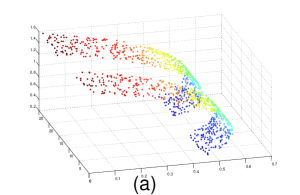
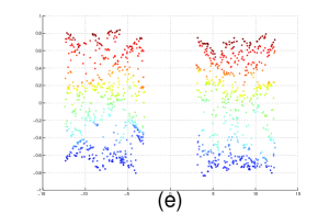
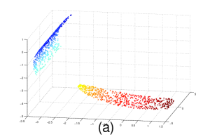
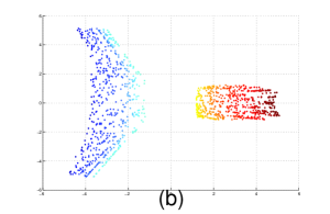
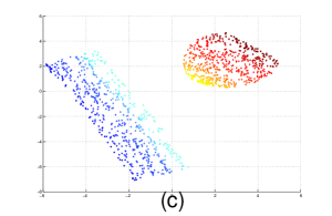
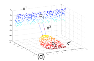
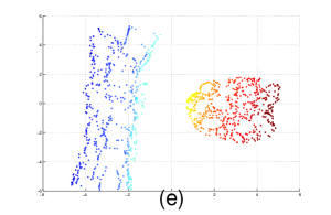
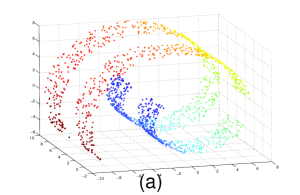
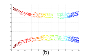
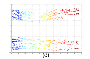
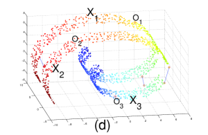
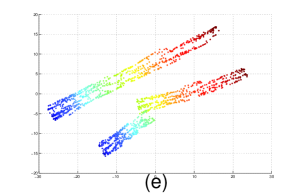
In this subsection, we compare k-CC Isomap, M-Isomap and the revised D-C Isomap on three 3-D data sets. It should be noted that during all experiments, the size of the neighborhood is chosen corresponding to the best performance of each algorithm.

Fig. 3(a) is a two-manifolds data set with $N=1200$ data points, and the data set is generated by the following matlab code:
 
t=(1*pi/6)*(1+2*rand(1,N)); xx=t.*cos(t);yy=t.*sin(t); zz =[unifrnd(1,10,1,N/2) unifrnd(16,25,1,N/2)]; X=[xx;zz;yy];
 

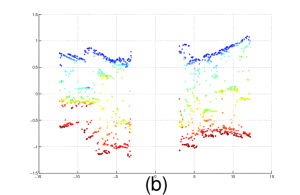
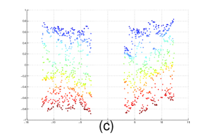
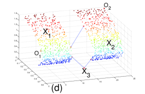
It can be seen that each data manifold is intrinsically a rectangular region with 600 data points. Fig. 3(b) shows the result got by k-CC Isomap, whose neighborhood graph is constructed by using 8-CC method. It can be seen that the embedding shrinks along the edges in low dimensional space and edges of the embedding turn into noisy. Fig. 3(c) shows the result got by M-Isomap method with neighborhood size $k=8$. As it can be seen, each of data manifold is exactly unrolled, and the inter-manifolds distance is precisely preserved. Fig. 3(d) illustrates the initialization step of the revised D-C Isomap algorithm. First, two data manifolds $X^{1}$ and $X^{2}$ are identified. Then the third data cluster $X^{3}$ is constructed, where the parameter $\lambda=0.1$. Finally, centers $O_{1}$ and $O_{2}$ of the data manifolds are computed by referring to the nearest neighbors. The center of $X^{3}$ is also the data point $X^{3}$. Fig. 3(e) shows the result of the revised D-C Isomap method. It is can be seen that the embedding exactly preserves both the intra-manifold distances and inter-manifolds distances.

Fig. 4(a) is another two-manifolds data set with $N=1200$ data points, and the data set is generated by the following matlab code:
 
t=[unifrnd(pi*11/12,pi*14/12,1,N/2)     unifrnd(pi*16/12,pi*19/12,1,N/2)]; xx=t.*cos(tt);yy=t.*sin(tt); zz=unifrnd(1,25,1,N); Y = [xx;zz;yy];
 
Each data manifold has 600 data points. One data manifold is a rectangular region and another data manifold is a round region. Fig. 4(b) shows the result got by k-CC Isomap with neighborhood size $k=10$. It can be seen that the rectangular region bent outwards and the round region is prolonged. Fig. 4(c) shows the result got by M-Isomap method with the neighborhood size $k=8$. As it can be seen, every data manifolds is exactly unrolled, and the inter-manifolds relationship is precisely preserved. Fig. 4(d) illustrates the initialization step of the revised D-C Isomap algorithm. The parameter $\lambda=0.5$ for production of the new cluster $X^{3}$. Fig. 4(e) shows the result of the revised D-C Isomap method with neighborhood size $k=5$. It is can be seen that the embedding exactly preserves both the intra-manifold distances and inter-manifolds distances.

Fig. 5(a) shows a three-manifolds data set with $N=1600$ data points on the Swiss roll manifold. The data set is generated by the following matlab code:
 
t1 = [unifrnd(pi*5/6,pi*16/12,1,N/4)]; t2 = [unifrnd(pi*18/12,pi*12/6,1,N/4)]; t3=(5*pi/6)*(1+7/5*rand(1,N/2)); a1=t1.*cos(t1); b1=t1.*sin(t1); c1=[unifrnd(-1,3,1,N/4)]; a2=t2.*cos(t2); b2=t2.*sin(t2); c2=[unifrnd(-1,3,1,N/4)]; a3=t3.*cos(t3); b3=t3.*sin(t3); c3=[unifrnd(6,10,1,N/2)]; x1=[a1;c1;b1]; x2=[a2;c2;b2]; x3=[a3;c3;b3] Z=[x1 x2 x3];
 
There are three rectangular regions on the Swiss roll manifold. The longest data manifold has 800 data points, the other two shorter data manifolds each contain 400 data points. Fig. 5(b) shows the result got by k-CC Isomap with neighborhood size $k=10$. Because of bad approximation of the inter-manifolds geodesics, edges of the data manifolds bend outwards. Fig. 5(c) shows the result got by M-Isomap method, where the neighborhood size $k$ is set to be $8$. As it can be seen, all data manifolds are exactly unrolled, and the inter-manifolds relationships of the three data manifolds are faithfully preserved. Fig. 5(d) illustrates the initiation step of the revised D-C Isomap algorithm. Fig. 5(e) shows the result of the revised D-C Isomap method. It is can be seen that the embedding do not exactly preserve the inter-manifolds distances. That is because the shape of the data manifolds are very narrow. The selected reference data points can not efficiently relocate each piece of data manifold.

V-B Real world data sets

Figure 6: (a) the face data set of five people. (b) the result by PCA. (c) the result by k-CC Isomap. (d) the result by M-Isomap. (e) the result by D-C Isomap.

Figure 7: (a) Data points of the teapot data set, ’$\oblong$’ stands for teapot vertical view rotation, ’$\bigtriangleup$’ stands for the teapot side view back-forth rotation and ’$\bigcirc$’ stand for teapot side view rotation. (b) The result of Isomap on the teapot vertical view rotation set. (c) The result of Isomap on the teapot side view back-forth rotation set. (d) The result of Isomap on the teapot side view rotation set. (e) The result of PCA on teapot data set. (f) The result of k-CC Isomap on teapot data set. (g) The result of M-Isomap on teapot data set. (h) The result of D-C Isomap on teapot data set.

Figure 8: (a) data points of the IsoFACE and teapot data set, where ’$\bullet$’ stands for the IsoFACE data set and ’$\bigcirc$’ stands for the teapot vertical view data set. (b) the result of Isomap on IsoFACE data set. (c) the result of Isomap on teapot vertical view data set. (d) the result of k-CC Isomap on IsoFACE and teapot data set. (e) the result of M-Isomap on IsoFACE and teapot data set. (f) the result of D-C Isomap on IsoFACE and teapot data set.

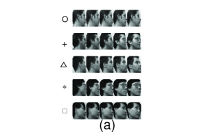
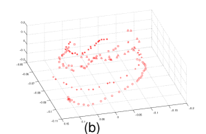
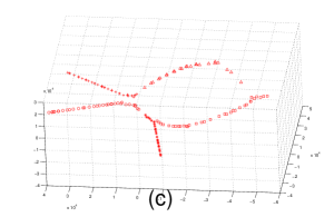
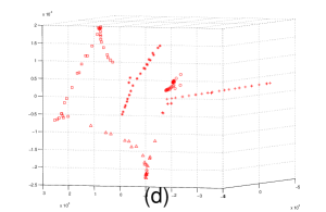
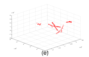
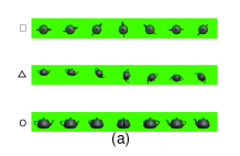
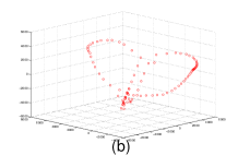
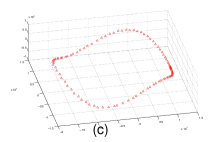
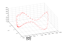
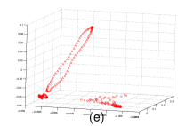
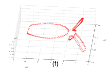
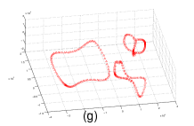
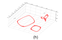
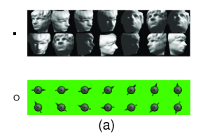
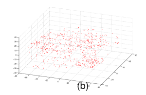
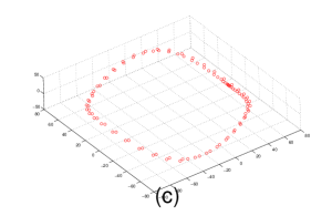
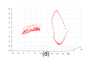
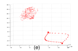
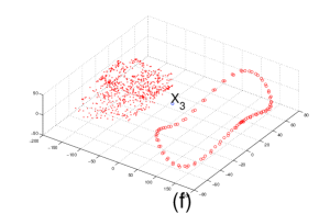
Fig. 6(a) shows some samples of the faces data [38] which contains face images of five persons . The data set consists of 153 images and has 34, 35, 26, 24, 34 images corresponding to each face. These images are gray scale with resolution of 112$\times$92. They are transformed into vectors in 10304-dimensional Euclidean space. In order to show the inter-manifolds relationship with more details, we embed the data into 3-dimensional space. Fig. 6(b) is the three dimensional embedding by PCA method. It can be observed that data manifolds of faces are mixed up, and the intra-face information is also not preserved. Fig. 6(c) is the result got by k-CC Isomap method with $k=3$. As it can be seen, although the data points are clustered, their inter-face distances are not well preserved. The five lines mix up at one of their endings. Fig. 6(d) shows the result got by M-Isomap method with $k=3$. Due to the limitation of k-NN method in clustering, only two data manifolds are identified. Although the data set is not well clustered, the result of M-Ismap shows that the low dimensional embedding can be separated up easily. Fig. 6(e) is the result got by the original D-C Isomap method, where the faces are spit up beforehand. The circumcenters are used as their centers. However, as it can be seen, two faces are mixed up.

Fig. 7(a) shows some samples of the teapot data set with 300 data points, where ’$\boxempty$’ stands for the teapot bird-view images, ’$\Delta$’ stands for the teapot back-forth rotation images and ’$\bigcirc$’ stands for the teapot side-view images. Each of the images is an 80$\times$60$\times$3 RGB colored picture, i.e. a vector in 14400 dimensional input space. Because the data points do not distribute on a single global manifold, this problem will poses a great challenge to classical manifold learning methods. The experiment shows that the three data manifolds can be identified by k-CC method. In order to show their exact embedding, Fig. 7(b)-(d) present the embedding of each data manifold by classical Isomap with neighborhood size $k=3$. Fig. 7(e) shows the result got by PCA method. It can be seen that the data set is clustered, but the shape of each embedding is deformed because of the linear characteristic of the PCA method. Fig. 7(f) is the result got by k-CC Isomap method with neighborhood size $k=3$. The bad approximations of inter-manifolds geodesics lead to the deformation of the embedding in low dimensional space. Fig. 7(g) shows the result by M-Isomap method with neighborhood size $k=3$. The data set is clearly clustered and intra-manifolds relationships are exactly preserved. Fig. 7(h) shows the result got by revised D-C Isomap method with neighborhood size $k=3$. It can be seen that the revised algorithm produces a satisfying result.

Fig. 8(a) shows samples of the IsoFACE and teapot rotation bird-view data. IsoFACE data consists of 698 images and each image is a 64$\times$64 (4096-dimensional) gray scale picture. As the input dimension of IsoFACE data set is different from the input dimension of teapot data set, we increase the dimension of IsoFACE set by adding zeros to the bottom of these vectors. The scale of the teapot data set should also be changed such that the scales of two embedding can be comparable. Teapot data vectors are divided by 100, i.e. the scale of teapot data points shrink to $\frac{1}{100}$ of its original ones. Fig. 8(b) is the 3-D embedding of IsoFACE by classical Isomap with neighborhood size k=5. Fig. 8(c) is the scaled teapot 3-D embedding got by classical Isomap with neighborhood size $k=5$. Fig. 8(d) is the result got by 5-CC Isomap method. We can see that the shape of IsoFACE data is distorted badly. Fig. 8(e) is the result got by M-Isomap method with neighborhood size k=5. The performance is significantly improved compared with k-CC Isomap. Fig. 8(f) is the result got by the revised D-C Isomap method.

V-C Discussion

TABLE III: The generalization performance of classical Isomap, k-CC Isomap, Original D-C Isomap, revised D-C Isomap and M-Isomap for multi-manifolds learning.

method	density	dimensionality	Isometric	generalization
classical	$\Delta$	$\Delta$	$\Delta$	$\Delta$
k-CC	$\bigcirc$	$\bigcirc$	$\Delta$	$\boxempty$
Original D-C	$\bigcirc$	$\bigcirc$	$\bigcirc$	$\boxempty$
revised D-C	$\bigcirc$	$\bigcirc$	$\bigcirc$	$\bigcirc$
Multi-	$\bigcirc$	$\bigcirc$	$\bigcirc$	$\bigcirc$

In our experiments, there are several important properties which should be considered:

1. As k-CC Isomap tries to preserve poor and good approximations of geodesics simultaneously, its low dimensional embedding is usually deformed. This method works well if each data manifold has comparable number of data points and the data manifolds can not be very far from each other, and the algorithm does not work well otherwise.

2. The revised D-C Isomap overcomes its original limitations, meanwhile, the robustness of the algorithm is also enhanced by adding a new cluster.

3. M-Isomap connects data manifolds with multiple edges, which can control the rotation of the low dimensional embedding, and at the same time, better preserve inter-manifolds distance. Like the D-C Isomap algorithm, it can also isometrically preserve intra-manifold geodesics and inter-manifolds distances.

To sum up, Table III shows the comparison of the general performance of the five versions of Isomap algorithms: classical Isomap, k-CC Isomap , Original D-C Isomap, revised D-C Isomap and M-Isomap. The labels ”$\Delta$” stands for poor performance, ”$\boxempty$” stands for not bad and ”$\bigcirc$” stands for good. Density means the generalize ability on manifolds with different density, i.e. different neighborhood sizes; dimensionality means the generalization ability on manifolds with different intrinsic dimensionality; isometric means the property of isometry in preserving the inter and intra-manifold relationship; finally the generalization means the overall generalization ability to learn data from multiple manifolds.

VI Conclusion

In this paper, the problem of multi-manifolds learning is presented and defined for the first time. A general procedure for isometric multi-manifolds learning is proposed. The procedure can be used to build multi-manifolds learning algorithms which are not only able to faithfully preserve intra-manifold geodesic distances, but also the inter-manifolds geodesic distances. M-Isomap is an implementation of the procedure and shows promising results in multi-manifolds learning. Compared with k-CC Isomap, it has the advantage of low computational complexity. With the procedure, the revised D-C Isomap becomes more effective in learning multi-manifolds data sets. Future work will be conducted on the applications of the multi-manifolds learning algorithms.

References

- [1] I. T. Jolliffe, “Principal Component Analysis,” Springer-Varlag, New York, 1989. ISBN 0-387-96269-7
- [2] T. F. Cox, M. A. Cox, “Multidimensional Scaling,” Chapman & Hall, London, 2001. ISBN 1-58488-094-5.
- [3] Eric Mjolsness, Dennis DeCoste, “Machine Learning for Science: State of the Art and Future Prospects,” Science, vol. 293, pp. 2051-2055, Sep. 2001.
- [4] J.B. Tenenbaum, V. de Sliva, and J. C. Landford, “A global geometric framework for nonlinear dimensionality reduction,” Science, vol. 290, pp. 2319-2323, Dec. 2000.
- [5] S. T. Roweis and L. K. Saul, “Nonlinear dimensionality reduction by local linear embedding,” Science, vol. 290, pp. 2323-2326, Dec. 2000.
- [6] H. S. Seung, D. D. Lee, “The manifold ways of perception,” Science, vol. 290, pp. 2268-2269, Dec. 2000.
- [7] M. Belkin and P. Niyogi, “Laplacian Eigenmaps for Dimensionality Reduction and Data Representation,” Neural Computation, vol. 15, no 6, pp. 1373-1396, June 2003.
- [8] D. Donoho, C. Grimes, “Hessian Eigenmaps: New Locally Linear Embedding Techniques for High-Dimensional Data,” Proc. National Academy of Sciences, vol. 100, no. 10, pp. 5591-5596, 2003.
- [9] Zhenyue Zhang, Hongyuan Zha, “Principal Manifolds and Nonlinear Dimensionality Reduction via Tangent Space Alignment,” SIAM Journal on Scientific Computing , vol. 26, issue. 1, pp. 313-338, 2005.
- [10] R. R. Coifman, S. Lafon, A. B. Lee, M. Maggoni, B. Nadler, F. Warner, S. W. Zuck, “Geometric diffusions as a tool for harmonic analysis and structure definition of data: Diffusion maps,” Proc. National Academy of Sciences, vol. 102, no. 21, pp. 7426-7431, May. 2005.
- [11] Tong Lin, Hongyuan Zha, “Riemannian Manifold Learning,” IEEE Trans. Pattern Analysis and Machine Intelligence, vol. 30, no5, pp. 796-809, May. 2008.
- [12] Hongyuan Zha, Zhenyue Zhang, “Continuum Isomap for manifold learning,” Computational Statistics & Data Analysis, vol. 52, issue. 1, pp. 184-200, Sep. 2007.
- [13] Martin H. C. Law, A. K. Jain, “Incremental Nonlinear Dimensionality Reduction by Manifold Learning,” IEEE Trans. Pattern Analysis and Machine Intelligence, vol. 28, no. 3, pp. 377-391, March. 2006.
- [14] M. Bernstein, V. de Silva, J. C. Langford, J. B. Tenenbaum, “Graph approximations to geodesics on embedded manifolds,” Technical report, Dept. of Psychology, Stanford Univ., Dec. 2000.
- [15] Maurizio Filippone, Francesco Camastra, Francesco Masulli, Stefano Rovetta, “A survey of kernel and spectral methods for clustering,” Pattern Recognition, vol. 41, pp. 176-190, May. 2007.
- [16] Ming-Hsuan Yang, “Extended Isomap for Pattern Classification,” ICPR 2002: Proceedings - International Conference on Pattern Recognition, vol. 3, pp. 30615, Aug. 2002
- [17] Xiaofei He, Shuicheng Yan, Tuxiao Hu, P. Niyogi, Hong-jiang Zhang, “Face recognition using Laplacianfaces,” IEEE Trans. Pattern Analysis and Machine Intelligence, vol. 27, issue:3, pp. 328-340, March. 2005.
- [18] M. Belkin, V. Sindhwani, and P. Niyogi, “Manifold Regularization: a Geometric Framework for Learning from Examples,” Journal of Machine Learning Research, vol. 7, pp. 2399-2434, Dec. 2006.
- [19] Xin Geng, De-Chuan Zhang, Zhi-hua Zhou, “Supervised nonlinear dimensionality reduction for visualization and classification,” IEEE Trans on Systems, Man, and Cybernetics Part B, vol. 35, no. 6, pp. 1098-1107, Dec 2005.
- [20] O. C. Jenkins, Maja J. Mataric, “A Spatio-temporal Extension to Isomap Nonlinear Dimension Reduction,” ACM. Proc. 21st Int’l Conf. on Machine learning, vol. 69, pp. 56-66, 2004
- [21] A. Rahimi, B. Recht, T. Darrell, “Learning to Transform Time Series with a Few Examples ,” IEEE Trans. Pattern Analysis and Machine Intelligence, vol. 29, no. 10, pp. 1759-1775, Oct. 2007.
- [22] J.B. Tenenbaum, V. de Sliva, and J. C. Landford “Respond to Comments on the Isomap Algorithm and Topological Stability,” Sciences, vol. 295, no. 5552, pp. 7, Jan. 2002.
- [23] Yiming Wu, Kap Luk Chan “An Extended Isomap Algorithm for Learning Multi-Class Manifold,” Proceedings of 2004 International Conference on Machine Learning and Cybernetics, vol. 6, pp. 3429-3433, Aug. 2004.
- [24] Deyu Meng, Yee Leung, Tung Fung, Zongben Xu “Nonlinear Dimensionality Reduction of Data Lying on the Multicluster Manifold,” IEEE Trans on Systems, Man, and Cybernetics Part B, vol. 38, issue. 4, pp. 1111-1122. Aug. 2008.
- [25] Bo Li, De-Shuang Huang, Chao Wang, Kun-Hong Liu “Feature extraction using constrained maximum variance mapping,” Pattern Recognition, vol. 41, pp. 3287-3294. May. 2008.
- [26] Li Yang, “K-Edge Connected Neighborhood Graph for Geodesic Distance Estimation and Nonlinear Projection,” Proceedings of the Pattern Recognition, 17th International Conference on (ICPR’04), vol. 1, pp. 196-199. 2004.
- [27] Li Yang, “Building k Edge-Disjoint Spanning Trees of Minimum Total Length for Isometric Data Embedding,” IEEE Trans. Pattern Analysis and Machine Intelligence, vol. 27, no. 10, pp. 1680-1683, Oct. 2005.
- [28] Li Yang, “Building k Edge-connected neighborhood graph for distance-based data projection,” Pattern Recognition Letters, vol. 26, issue. 13, pp. 2015-2021, Oct. 2005.
- [29] Li Yang, “Building k-Connected Neighborhood Graphs for Isometric Data Embedding,” IEEE Trans. Pattern Analysis and Machine Intelligence, vol. 28, issue. 5, pp. 827-831, May. 2006.
- [30] Dongfang Zhao, Li Yang, “Incremental Construction of Neighborhood Graphs for Nonlinear Dimensionality Reduction,” International Conference on Pattern Recognition, vol. 28, issue. 5, pp. 827-831, May. 2006.
- [31] Dongfang Zhao, Li Yang, “Incremental Isometric Embedding of High-Dimensional Data Using Connected Neighborhood Graphs,” IEEE Trans. Pattern Analysis and Machine Intelligence, vol. 31, no. 1, pp. 86-98, Jan. 2009.
- [32] O. Samko, A. D. Marshall, P. L. Rosin “ Selection of the optimal parameter value for the Isomap algorithm,” Pattern Recognition Letters vol. 27, issue. 9, pp. 968-979, Feb. 2006.
- [33] R. Xu, D. Wunsch II, ”Survey of clustering algorithms,” IEEE Trans on Neural Networks, vol. 16, no. 3, pp. 645-678, May. 2005.
- [34] F. Camastra and A. Vinciarelli, ”Estimating the intrinsic dimension of data with a fractal-based approach,” IEEE Trans. Pattern Analysis and Machine Intelligence vol. 24, no. 10, pp. 1404-1407, Oct. 2002.
- [35] E. Levina and P. J. Bickel “Maximum likelihood estimation of intrinsic dimension,” NIPS 04: Neural Information Processing Systems
- [36] D.J.C. MacKay and Z. Ghahramani, ”Comments on ’Maximum likelihood estimation of intrinsic dimension’ by E. Levina and P. Bickel (2005),” in: http://www.inference.phy.cam.ac.uk/mackay/dimension/
- [37] Mingyu Fan, Hong Qiao, Bo Zhang, ”Intrinsic dimension estimation of manifolds by incising balls,” Pattern Recognition vol. 42, issue. 5, pp. 780-787, May. 2009.
- [38] B Graham and Nigel M Allinson, ”Characterizing Virtual Eigensignatures for General Purpose Face Recognition”, In H. Wechsler, P. J. Phillips, V. Bruce, and F. Fogelman-Soulie and T. S. Huang (eds): ”Face Recognition: From Theory to Applications;” NATO ASI Series F, Computer and Systems Sciences, Vol. 163; pp 446-456, 1998.
- [39] D. Kushnir, M. Galun, A. Brandt “Fast multiscale clustering and manifold identification,” Pattern Recognition vol. 28, issue. 10, pp. 1876-1891, Oct. 2006.