A new approach to
the Baker-Campbell-Hausdorff expansion
A.V.Bratchikov
Abstract
For noncommutative variables x , y 𝑥 𝑦
x,y log ( e x e y ) superscript 𝑒 𝑥 superscript 𝑒 𝑦 \log(e^{x}e^{y}) x + y 𝑥 𝑦 x+y x − y . 𝑥 𝑦 x-y.
Let L 𝐿 L f ( x , y ) 𝑓 𝑥 𝑦 f(x,y)
f ( x , y ) = log ( e x e y ) . 𝑓 𝑥 𝑦 superscript 𝑒 𝑥 superscript 𝑒 𝑦 f(x,y)=\log(e^{x}e^{y}).
The expansion of f ( x , y ) 𝑓 𝑥 𝑦 f(x,y) x , y 𝑥 𝑦
x,y
f ( x , y ) = ∑ m = 1 ∞ p m ( x , y ) , 𝑓 𝑥 𝑦 superscript subscript 𝑚 1 subscript 𝑝 𝑚 𝑥 𝑦 \displaystyle f(x,y)=\sum_{m=1}^{\infty}p_{m}(x,y), (1)
where p m ( x , y ) subscript 𝑝 𝑚 𝑥 𝑦 p_{m}(x,y) m 𝑚 m x 𝑥 x y . 𝑦 y. p m ( x , y ) subscript 𝑝 𝑚 𝑥 𝑦 p_{m}(x,y) x , y 𝑥 𝑦
x,y x 𝑥 x y . 𝑦 y. 1 p m ( x , y ) subscript 𝑝 𝑚 𝑥 𝑦 p_{m}(x,y) [1 ] .
The BCH series plays an important role in theoretical physics (see e.g.
[2 ] ,
[3 ] ). Recent applications are connected with deformation quantization of Poisson manifolds [4 ] , [5 ] .
For x + y = 0 𝑥 𝑦 0 x+y=0 f ( x , y ) = 0 , 𝑓 𝑥 𝑦 0 f(x,y)=0, f ( x , y ) 𝑓 𝑥 𝑦 f(x,y)
f ( x , y ) = ∑ m = 1 ∞ q m ( x − y , x + y ) , 𝑓 𝑥 𝑦 superscript subscript 𝑚 1 subscript 𝑞 𝑚 𝑥 𝑦 𝑥 𝑦 \displaystyle f(x,y)=\sum_{m=1}^{\infty}q_{m}(x-y,x+y), (2)
where q m ( x − y , x + y ) subscript 𝑞 𝑚 𝑥 𝑦 𝑥 𝑦 q_{m}(x-y,x+y) m 𝑚 m x + y . 𝑥 𝑦 x+y.
f ( ( x + y ) / 2 , ( x − y ) / 2 ) = ∑ m = 1 ∞ q m ( y , x ) . 𝑓 𝑥 𝑦 2 𝑥 𝑦 2 superscript subscript 𝑚 1 subscript 𝑞 𝑚 𝑦 𝑥 \displaystyle f((x+y)/2,(x-y)/2)=\sum_{m=1}^{\infty}q_{m}(y,x).
The aim of this paper is to find an expression for q m subscript 𝑞 𝑚 q_{m}
For x , y ∈ L 𝑥 𝑦
𝐿 x,y\in L
ψ ( t , x , y ) = log ( e t x e t y ) , t ∈ ℝ . formulae-sequence 𝜓 𝑡 𝑥 𝑦 superscript 𝑒 𝑡 𝑥 superscript 𝑒 𝑡 𝑦 𝑡 ℝ \psi(t,x,y)=\log(e^{tx}e^{ty}),\qquad t\in\mathbb{R}.
Let k ( z ) 𝑘 𝑧 k(z) ℂ ℂ \mathbb{C} k ( z ) = z / ( 1 − e − z ) − z / 2 . 𝑘 𝑧 𝑧 1 superscript 𝑒 𝑧 𝑧 2 k(z)=z/(1-e^{-z})-z/2. [6 ] that
k ( z ) = 1 + ∑ p = 1 ∞ k 2 p z 2 p , 𝑘 𝑧 1 superscript subscript 𝑝 1 subscript 𝑘 2 𝑝 superscript 𝑧 2 𝑝 \displaystyle k(z)=1+\sum_{p=1}^{\infty}k_{2p}z^{2p}, (3)
where k 2 p = B 2 p / ( 2 p ) ! , subscript 𝑘 2 𝑝 subscript 𝐵 2 𝑝 2 𝑝 k_{2p}=B_{2p}/(2p)!, B 2 p subscript 𝐵 2 𝑝 B_{2p}
B 2 = 1 6 , B 4 = − 1 30 , B 6 = 1 42 , … . formulae-sequence subscript 𝐵 2 1 6 formulae-sequence subscript 𝐵 4 1 30 subscript 𝐵 6 1 42 …
B_{2}=\frac{1}{6},\quad B_{4}=-\frac{1}{30},\quad B_{6}=\frac{1}{42},\ldots.
Then ψ ( t , x , y ) 𝜓 𝑡 𝑥 𝑦 \psi(t,x,y) [7 ]
d ψ d t = k ( a d ψ ) ( x + y ) + 1 2 [ x − y , ψ ] 𝑑 𝜓 𝑑 𝑡 𝑘 𝑎 𝑑 𝜓 𝑥 𝑦 1 2 𝑥 𝑦 𝜓 \displaystyle\frac{d\psi}{dt}=k(ad\psi)(x+y)+\frac{1}{2}[x-y,\psi] (4)
with the initial condition
ψ ( 0 , x , y ) = 0 . 𝜓 0 𝑥 𝑦 0 \psi(0,x,y)=0.
Equation (4
ψ ( t ) = e t 2 a d ( x − y ) ∫ 0 t e − τ 2 a d ( x − y ) k ( a d ψ ( τ ) ) ( x + y ) 𝑑 τ . 𝜓 𝑡 superscript 𝑒 𝑡 2 𝑎 𝑑 𝑥 𝑦 superscript subscript 0 𝑡 superscript 𝑒 𝜏 2 𝑎 𝑑 𝑥 𝑦 𝑘 𝑎 𝑑 𝜓 𝜏 𝑥 𝑦 differential-d 𝜏 \displaystyle\psi(t)=e^{\frac{t}{2}ad(x-y)}\int_{0}^{t}e^{-\frac{\tau}{2}ad(x-y)}k(ad\psi(\tau))(x+y)d\tau. (5)
This can be written in the form
ψ = ψ 0 + ∑ n = 1 ∞ g 2 n ( ψ ) , 𝜓 subscript 𝜓 0 superscript subscript 𝑛 1 subscript 𝑔 2 𝑛 𝜓 \displaystyle\psi=\psi_{0}+\sum_{n=1}^{\infty}g_{2n}(\psi), (6)
where
ψ 0 = e t 2 a d ( x − y ) ∫ 0 t e − τ 2 a d ( x − y ) ( x + y ) 𝑑 τ = ∑ n = 0 ∞ t n + 1 ( n + 1 ) ! 2 n ( a d ( x − y ) ) n ( x + y ) , subscript 𝜓 0 superscript 𝑒 𝑡 2 𝑎 𝑑 𝑥 𝑦 superscript subscript 0 𝑡 superscript 𝑒 𝜏 2 𝑎 𝑑 𝑥 𝑦 𝑥 𝑦 differential-d 𝜏 superscript subscript 𝑛 0 superscript 𝑡 𝑛 1 𝑛 1 superscript 2 𝑛 superscript 𝑎 𝑑 𝑥 𝑦 𝑛 𝑥 𝑦 \displaystyle\psi_{0}=e^{\frac{t}{2}ad(x-y)}\int_{0}^{t}e^{-\frac{\tau}{2}ad(x-y)}(x+y)d\tau=\sum_{n=0}^{\infty}\frac{t^{n+1}}{(n+1)!2^{n}}\left(ad(x-y)\right)^{n}(x+y),
g 2 n ( ψ ) = k 2 n e t 2 a d ( x − y ) ∫ 0 t e − τ 2 a d ( x − y ) ( a d ψ ( τ ) ) 2 n ( x + y ) 𝑑 τ . subscript 𝑔 2 𝑛 𝜓 subscript 𝑘 2 𝑛 superscript 𝑒 𝑡 2 𝑎 𝑑 𝑥 𝑦 superscript subscript 0 𝑡 superscript 𝑒 𝜏 2 𝑎 𝑑 𝑥 𝑦 superscript 𝑎 𝑑 𝜓 𝜏 2 𝑛 𝑥 𝑦 differential-d 𝜏 g_{2n}(\psi)=k_{2n}e^{\frac{t}{2}ad(x-y)}\int_{0}^{t}e^{-\frac{\tau}{2}ad(x-y)}\left(ad\psi(\tau)\right)^{2n}(x+y)d\tau.
Let us introduce the
functions
⟨ … . ⟩ 2 n : L 2 n → L , n = 1 , 2 , … , \displaystyle\langle\ldots.\rangle_{2n}:{L}^{2n}\to L,\quad n=1,2,\ldots,
defined for v 1 , … , v 2 n ∈ L subscript 𝑣 1 … subscript 𝑣 2 𝑛
𝐿 v_{1},\ldots,v_{2n}\in L
⟨ v 1 , … , v 2 n ⟩ 2 n = ∂ ∂ α 1 … ∂ ∂ α 2 n g 2 n ( α 1 v 1 + … + α 2 n v 2 n ) . subscript subscript 𝑣 1 … subscript 𝑣 2 𝑛
2 𝑛 subscript 𝛼 1 … subscript 𝛼 2 𝑛 subscript 𝑔 2 𝑛 subscript 𝛼 1 subscript 𝑣 1 … subscript 𝛼 2 𝑛 subscript 𝑣 2 𝑛 \displaystyle\langle v_{1},\ldots,v_{2n}\rangle_{2n}=\frac{\partial}{\partial\alpha_{1}}\ldots\frac{\partial}{\partial\alpha_{2n}}g_{2n}(\alpha_{1}v_{1}+\ldots+\alpha_{2n}v_{2n}). (7)
The function ⟨ v 1 , … , v 2 n ⟩ 2 n subscript subscript 𝑣 1 … subscript 𝑣 2 𝑛
2 𝑛 \langle v_{1},\ldots,v_{2n}\rangle_{2n} v i , subscript 𝑣 𝑖 v_{i}, 7
⟨ v , … , v ⟩ 2 n = ( 2 n ) ! g 2 n ( v ) . subscript 𝑣 … 𝑣
2 𝑛 2 𝑛 subscript 𝑔 2 𝑛 𝑣 \displaystyle\langle v,\ldots,v\rangle_{2n}={(2n)!}g_{2n}(v).
Then equation (6
ψ = k ψ 0 + k ∑ n = 1 ∞ 1 ( 2 n ) ! ⟨ ψ , … , ψ ⟩ 2 n . 𝜓 𝑘 subscript 𝜓 0 𝑘 superscript subscript 𝑛 1 1 2 𝑛 subscript 𝜓 … 𝜓
2 𝑛 \displaystyle\psi=k\psi_{0}+k\sum_{n=1}^{\infty}\frac{1}{(2n)!}\langle\psi,\ldots,\psi\rangle_{2n}. (8)
Here we introduced an auxiliary parameter k 𝑘 k x + y . 𝑥 𝑦 x+y. 1 . 1 1.
To describe a solution of equation (8
P i 1 … i 2 n m : L m → L m − 2 n + 1 , : subscript superscript 𝑃 𝑚 subscript 𝑖 1 … subscript 𝑖 2 𝑛 → superscript 𝐿 𝑚 superscript 𝐿 𝑚 2 𝑛 1 P^{m}_{i_{1}\ldots i_{2n}}:L^{m}\to L^{m-2n+1},
m ≥ 2 , 1 ≤ i 1 < … < i 2 n ≤ m , formulae-sequence 𝑚 2 1 subscript 𝑖 1 … subscript 𝑖 2 𝑛 𝑚 m\geq 2,1\leq i_{1}<\ldots<i_{2n}\leq m,
P i 1 … i 2 n m ( v 1 , … , v m ) = ( h ⟨ v i 1 , … , v i 2 n ⟩ 2 n , v 1 , … , v ^ i 1 , … , v ^ i 2 n , … , v m ) , subscript superscript 𝑃 𝑚 subscript 𝑖 1 … subscript 𝑖 2 𝑛 subscript 𝑣 1 … subscript 𝑣 𝑚 ℎ subscript subscript 𝑣 subscript 𝑖 1 … subscript 𝑣 subscript 𝑖 2 𝑛
2 𝑛 subscript 𝑣 1 … subscript ^ 𝑣 subscript 𝑖 1 … subscript ^ 𝑣 subscript 𝑖 2 𝑛 … subscript 𝑣 𝑚 \displaystyle P^{m}_{i_{1}\ldots i_{2n}}(v_{1},\ldots,v_{m})=(h\langle v_{i_{1}},\ldots,{v}_{i_{2n}}\rangle_{2n},v_{1},\ldots,\widehat{v}_{i_{1}},\ldots,\widehat{v}_{i_{2n}},\ldots,v_{m}),
where v ^ ^ 𝑣 \widehat{v} v 𝑣 {v} v ∈ L 𝑣 𝐿 v\in L
v = P I s n s … P I 2 m − n 1 + 1 P I 1 m ( v 1 , … , v m ) 𝑣 subscript superscript 𝑃 subscript 𝑛 𝑠 subscript 𝐼 𝑠 … subscript superscript 𝑃 𝑚 subscript 𝑛 1 1 subscript 𝐼 2 subscript superscript 𝑃 𝑚 subscript 𝐼 1 subscript 𝑣 1 … subscript 𝑣 𝑚 \displaystyle v=P^{n_{s}}_{I_{s}}\ldots P^{m-n_{1}+1}_{I_{2}}P^{m}_{I_{1}}(v_{1},\ldots,v_{m}) (9)
for some I 1 = ( i 1 1 , … , i n 1 1 ) , I 2 = ( i 1 2 , … , i n 2 2 ) , … , I s = ( i 1 s , … , i n s s ) , n 1 + … + n s − s + 1 = m , formulae-sequence subscript 𝐼 1 superscript subscript 𝑖 1 1 … subscript superscript 𝑖 1 subscript 𝑛 1 formulae-sequence subscript 𝐼 2 subscript superscript 𝑖 2 1 … subscript superscript 𝑖 2 subscript 𝑛 2 …
formulae-sequence subscript 𝐼 𝑠 subscript superscript 𝑖 𝑠 1 … subscript superscript 𝑖 𝑠 subscript 𝑛 𝑠 subscript 𝑛 1 … subscript 𝑛 𝑠 𝑠 1 𝑚 I_{1}=(i_{1}^{1},\ldots,i^{1}_{n_{1}}),I_{2}=(i^{2}_{1},\ldots,i^{2}_{n_{2}}),\ldots,I_{s}=(i^{s}_{1},\ldots,i^{s}_{n_{s}}),n_{1}+\ldots+n_{s}-s+1=m, v 𝑣 v ( v 1 , … , v m ) . subscript 𝑣 1 … subscript 𝑣 𝑚 (v_{1},\ldots,v_{m}). v 𝑣 v v . 𝑣 v.
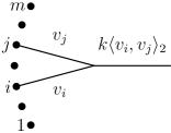
Each descendant can be represented by a diagram.
In this diagram an element of L 𝐿 L . A product
( v 1 , … , v 2 n ) → k ⟨ v 1 , … , v 2 n ⟩ 2 n → subscript 𝑣 1 … subscript 𝑣 2 𝑛 𝑘 subscript subscript 𝑣 1 … subscript 𝑣 2 𝑛
2 𝑛 (v_{1},\ldots,v_{2n})\to k\langle v_{1},\ldots,v_{2n}\rangle_{2n}
is represented by the vertex joining the line segments for v 1 , … , v 2 n , subscript 𝑣 1 … subscript 𝑣 2 𝑛
v_{1},\ldots,v_{2n}, k ⟨ v 1 , … , v 2 n ⟩ 2 n . 𝑘 subscript subscript 𝑣 1 … subscript 𝑣 2 𝑛
2 𝑛 k\langle v_{1},\ldots,v_{2n}\rangle_{2n}. v 1 , … , v m subscript 𝑣 1 … subscript 𝑣 𝑚
v_{1},\ldots,v_{m} k ⟨ v 1 , … , v 2 n ⟩ 2 n 𝑘 subscript subscript 𝑣 1 … subscript 𝑣 2 𝑛
2 𝑛 k\langle v_{1},\ldots,v_{2n}\rangle_{2n} P I m ( v 1 , … , v m ) subscript superscript 𝑃 𝑚 𝐼 subscript 𝑣 1 … subscript 𝑣 𝑚 P^{m}_{I}(v_{1},\ldots,v_{m})
P i j m ( v 1 , … , v m ) = ( k ⟨ v i , v j ⟩ 2 , v 1 , … , v ^ i , … , v ^ j , … , v m ) . subscript superscript 𝑃 𝑚 𝑖 𝑗 subscript 𝑣 1 … subscript 𝑣 𝑚 𝑘 subscript subscript 𝑣 𝑖 subscript 𝑣 𝑗
2 subscript 𝑣 1 … subscript ^ 𝑣 𝑖 … subscript ^ 𝑣 𝑗 … subscript 𝑣 𝑚 P^{m}_{ij}(v_{1},\ldots,v_{m})=(k\langle v_{i},v_{j}\rangle_{2},v_{1},\ldots,\widehat{v}_{i},\ldots,\widehat{v}_{j},\ldots,v_{m}).
The points labeled by 1 , … , m 1 … 𝑚
1,\ldots,m v 1 , … , v m . subscript 𝑣 1 … subscript 𝑣 𝑚
v_{1},\ldots,v_{m}. P i 1 … i 2 n m ( v 1 , … , v m ) subscript superscript 𝑃 𝑚 subscript 𝑖 1 … subscript 𝑖 2 𝑛 subscript 𝑣 1 … subscript 𝑣 𝑚 P^{m}_{i_{1}\ldots i_{2n}}(v_{1},\ldots,v_{m}) P I 1 n 1 ( v 1 , … , v m ) , P I 2 n 2 P I 1 n 1 ( v 1 , … , v m ) , … , v subscript superscript 𝑃 subscript 𝑛 1 subscript 𝐼 1 subscript 𝑣 1 … subscript 𝑣 𝑚 subscript superscript 𝑃 subscript 𝑛 2 subscript 𝐼 2 subscript superscript 𝑃 subscript 𝑛 1 subscript 𝐼 1 subscript 𝑣 1 … subscript 𝑣 𝑚 … 𝑣
P^{n_{1}}_{I_{1}}(v_{1},\ldots,v_{m}),P^{n_{2}}_{I_{2}}P^{n_{1}}_{I_{1}}(v_{1},\ldots,v_{m}),\ldots,v 9 v 𝑣 v
Figure 1: Diagram for P i j m ( v 1 , … , v m ) . subscript superscript 𝑃 𝑚 𝑖 𝑗 subscript 𝑣 1 … subscript 𝑣 𝑚 P^{m}_{ij}(v_{1},\ldots,v_{m}).
Let us introduce a family of functions
⟨ … ⟩ : L m → L , m = 1 , 2 , … , : delimited-⟨⟩ … formulae-sequence → superscript 𝐿 𝑚 𝐿 𝑚 1 2 …
\langle\ldots\rangle:{L}^{m}\to L,\qquad m=1,2,\ldots,
such that for v 1 , … , v m ∈ V subscript 𝑣 1 … subscript 𝑣 𝑚
𝑉 v_{1},\ldots,v_{m}\in V ⟨ v 1 , … , v m ⟩ subscript 𝑣 1 … subscript 𝑣 𝑚
\langle v_{1},\ldots,v_{m}\rangle
⟨ v 1 , v 2 ⟩ = k ⟨ v 1 , v 2 ⟩ 2 , subscript 𝑣 1 subscript 𝑣 2
𝑘 subscript subscript 𝑣 1 subscript 𝑣 2
2 \displaystyle\langle v_{1},v_{2}\rangle=k\langle v_{1},v_{2}\rangle_{2},
⟨ v 1 , v 2 , v 3 ⟩ = k 2 ( ⟨ ⟨ v 1 , v 2 ⟩ 2 , v 3 ⟩ 2 + ⟨ ⟨ v 1 , v 3 ⟩ 2 , v 2 ⟩ 2 + ⟨ ⟨ v 2 , v 3 ⟩ 2 , v 1 ⟩ 2 ) . subscript 𝑣 1 subscript 𝑣 2 subscript 𝑣 3
superscript 𝑘 2 subscript subscript subscript 𝑣 1 subscript 𝑣 2
2 subscript 𝑣 3
2 subscript subscript subscript 𝑣 1 subscript 𝑣 3
2 subscript 𝑣 2
2 subscript subscript subscript 𝑣 2 subscript 𝑣 3
2 subscript 𝑣 1
2 \displaystyle\langle v_{1},v_{2},v_{3}\rangle=k^{2}\left(\langle\langle v_{1},v_{2}\rangle_{2},v_{3}\rangle_{2}+\langle\langle v_{1},v_{3}\rangle_{2},v_{2}\rangle_{2}+\langle\langle v_{2},v_{3}\rangle_{2},v_{1}\rangle_{2}\right).
A solution of equation (8 [8 ]
ψ = ⟨ e k ψ 0 ⟩ , 𝜓 delimited-⟨⟩ superscript 𝑒 𝑘 subscript 𝜓 0 \displaystyle\psi=\langle e^{k\psi_{0}}\rangle, (10)
where
⟨ e k ψ 0 ⟩ = ∑ n = 0 ∞ k n n ! ⟨ ψ 0 n ⟩ , delimited-⟨⟩ superscript 𝑒 𝑘 subscript 𝜓 0 superscript subscript 𝑛 0 superscript 𝑘 𝑛 𝑛 delimited-⟨⟩ superscript subscript 𝜓 0 𝑛 \displaystyle\langle e^{k\psi_{0}}\rangle=\sum_{n=0}^{\infty}\frac{k^{n}}{n!}\langle\psi_{0}^{n}\rangle,
⟨ ψ 0 n ⟩ delimited-⟨⟩ superscript subscript 𝜓 0 𝑛 \langle\psi_{0}^{n}\rangle 0 0 n = 0 , 𝑛 0 n=0,
⟨ ψ 0 n ⟩ = ⟨ ψ 0 , … , ψ 0 ⏟ n times ⟩ . delimited-⟨⟩ superscript subscript 𝜓 0 𝑛 delimited-⟨⟩ subscript ⏟ subscript 𝜓 0 … subscript 𝜓 0
n times \langle\psi_{0}^{n}\rangle=\langle\underbrace{\psi_{0},\ldots,\psi_{0}}_{\text{n times}}\rangle.
We write
ψ = ∑ n = 1 ∞ π n ( t , x − y , x + y ) . 𝜓 superscript subscript 𝑛 1 subscript 𝜋 𝑛 𝑡 𝑥 𝑦 𝑥 𝑦 \displaystyle\psi=\sum_{n=1}^{\infty}\pi_{n}(t,x-y,x+y). (11)
Here π n subscript 𝜋 𝑛 \pi_{n} n 𝑛 n x + y . 𝑥 𝑦 x+y. q m subscript 𝑞 𝑚 q_{m} 2
q m ( x − y , x + y ) = π m ( 1 , x − y , x + y ) . subscript 𝑞 𝑚 𝑥 𝑦 𝑥 𝑦 subscript 𝜋 𝑚 1 𝑥 𝑦 𝑥 𝑦 q_{m}(x-y,x+y)=\pi_{m}(1,x-y,x+y).
Using (10
π 1 = k ψ 0 , π 3 = k 3 24 e t 2 a d ( x − y ) ∫ 0 t e − τ 2 a d ( x − y ) ( a d ψ 0 ( τ ) ) 2 ( x + y ) 𝑑 τ , π 2 = π 4 = 0 . formulae-sequence subscript 𝜋 1 𝑘 subscript 𝜓 0 formulae-sequence subscript 𝜋 3 superscript 𝑘 3 24 superscript 𝑒 𝑡 2 𝑎 𝑑 𝑥 𝑦 superscript subscript 0 𝑡 superscript 𝑒 𝜏 2 𝑎 𝑑 𝑥 𝑦 superscript 𝑎 𝑑 subscript 𝜓 0 𝜏 2 𝑥 𝑦 differential-d 𝜏 subscript 𝜋 2 subscript 𝜋 4 0 \displaystyle\pi_{1}=k\psi_{0},\quad\pi_{3}=\frac{k^{3}}{24}e^{\frac{t}{2}ad(x-y)}\int_{0}^{t}e^{-\frac{\tau}{2}ad(x-y)}\left(ad\psi_{0}(\tau)\right)^{2}(x+y)d\tau,\quad\pi_{2}=\pi_{4}=0.
The function π n ( x − y , x + y ) subscript 𝜋 𝑛 𝑥 𝑦 𝑥 𝑦 \pi_{n}(x-y,x+y) 10 k 𝑘 k π n subscript 𝜋 𝑛 \pi_{n} r 𝑟 r s 𝑠 s r + s = n . 𝑟 𝑠 𝑛 r+s=n.
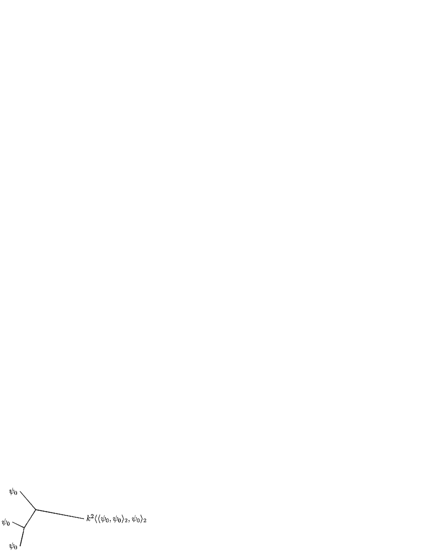
For example, the O ( k 5 ) 𝑂 superscript 𝑘 5 O(k^{5}) ψ 𝜓 \psi
π 5 = k 5 2 ⟨ ⟨ ψ 0 , ψ 0 ⟩ 2 , ψ 0 ⟩ 2 + k 5 24 ⟨ ψ 0 , ψ 0 , ψ 0 , ψ 0 ⟩ 4 . subscript 𝜋 5 superscript 𝑘 5 2 subscript subscript subscript 𝜓 0 subscript 𝜓 0
2 subscript 𝜓 0
2 superscript 𝑘 5 24 subscript subscript 𝜓 0 subscript 𝜓 0 subscript 𝜓 0 subscript 𝜓 0
4 \displaystyle\pi_{5}=\frac{k^{5}}{2}\langle\langle\psi_{0},\psi_{0}\rangle_{2},\psi_{0}\rangle_{2}+\frac{k^{5}}{24}\langle\psi_{0},\psi_{0},\psi_{0},\psi_{0}\rangle_{4}.
The diagram for k 2 ⟨ ⟨ ψ 0 , ψ 0 ⟩ 2 , ψ 0 ⟩ 2 superscript 𝑘 2 subscript subscript subscript 𝜓 0 subscript 𝜓 0
2 subscript 𝜓 0
2 k^{2}\langle\langle\psi_{0},\psi_{0}\rangle_{2},\psi_{0}\rangle_{2}
Figure 2: Diagram for k 2 ⟨ ⟨ ψ 0 , ψ 0 ⟩ 2 , ψ 0 ⟩ 2 . superscript 𝑘 2 subscript subscript subscript 𝜓 0 subscript 𝜓 0
2 subscript 𝜓 0
2 k^{2}\langle\langle\psi_{0},\psi_{0}\rangle_{2},\psi_{0}\rangle_{2}.
References
[1]
E.V.Dynkin,
Dokl.Akad.Nauk.SSSR, 57 (1947) 323-326.
[2]
L.C.Biedenharn and J.D.Louck, Angular momentum in quantum physics, Addison-Wesley, Reading (1981).
[3]
J.Zinn-Justin, Quantum field theory and critical phenomena, Clarendon Press, Oxford (1996).
[4]
V.Kathotia, Kontsevich’s universal formula for
deformation quantization and the Campbell-Baker-Hausdorff formula, Internat.J.Math. 11 (2000) 523-551.
[5]
A.V.Bratchikov, Deformation quantization of
Poisson manifolds in the derivative expansion, Int.J.Geom.Meth.Mod.Phys. 6 (2009) 219-224.
[6]
A.I.Markushevich, Theory of functions of a complex variable, Chelsea (1977).
[7]
V.S.Varadarajan, Lie groups, Lie algebras and their representations, Springer (1984).
[8]
A.V.Bratchikov, Perturbation theory for nonlinear equations, arXiv 0910.3924 [hep-th].