Exact modeling method for discrete finite metamaterial lens

Abstract

We describe an efficient rigorous model suitable for calculating the properties of finite metamaterial samples, which takes into account the discrete structure of metamaterials based on capacitively loaded ring resonators. We illustrate how this model applies specifically to a metamaterial lens employed in magnetic-resonant imaging. We show that the discrete model reveals the effects which can be missed by a continuous model based on effective parameters, and that the results are in close agreement with the experimental data.

I Introduction

For the last decade, metamaterials SolSha ; MarMarSor are in the focus of research attention in theoretical and applied electrodynamics. Even though no commonly accepted definition is available ML7 ; Sih07 , this research direction experiences a boom encompassing a wide span of areas ranging from microwave engineering to nonlinear optics. One of the well-known suggestions for applications was formulated as a “perfect lens” Pen00 , making use of negative effective material parameters and providing imaging with subwavelength resolution. The idea of super-resolution was subsequently analysed and developed in a number of ways SKR1 ; MTA4 ; MFM5 , and even realized in practice (speaking about three-dimensional systems) using split-ring resonators (SRRs) Fre5 ; FreMarJel08 , or transmission-line networks Grb5 ; AliTre07 .

Arguably the closest approach to practice offered by metamaterials, is related to magnetic resonance imaging (MRI). For example, rotational resonance of magnetoinductive waves SolZhuSyd06 was suggested for parametric amplification of MRI signals SymSolYou07 or enhanced detection with flexible ring resonators SymYouSol10 . Alternatively, applications based on ‘swiss-rolls’ WHP3 or wire media IkoBelSim06 channelling were put forward WHP3 ; RadGarCra09 . Naturally, superlens concept is also promising in this area: specifically for MRI, an isotropic lens based on capacitively loaded single ring resonators was designed and experimentally tested FreMarJel08 .

Such a metamaterial lens is intended to operate at the value of effective permeability $\mu=-1$. In theory, for modelling such metamaterials (based on SRRs), one can exploit an effective medium approach, taking care of numerous limitations related to general restrictions of homogenization Agr09 as well as to specific peculiarities caused by resonant nature of the structural elements Sim08 . Universally, all the structure details (size of the elements and lattice constants) must be much smaller than the wavelength; while the total number of elements in metamaterial should be sufficiently large to make homogenization meaningful. In addition, spatial dispersion effects can be rather remarkable in metamaterials, and impose further restrictions on effective medium treatment, prohibiting that in certain frequency bands Sim08 .

Unless one opts for a completely numerical homogenization method Sil07 , generally applicable to almost arbitrary structures, a model have to be developed to describe adequately the effective medium properties. Quite general approach Sim08 for homogenization of resonant metamaterials can be applied to a variety of metamaterials including those which combine different element types. However, this relies on the dipole approximation for the interaction of elements in the lattice, which may not be always valid. For example, mutual interaction of the circular currents close to each other significantly differs from dipole interaction, which becomes relevant for dense metamaterials. The first rigorous analysis of such metamaterials was given early in Ref. GLS2 , where the effective permeability has been derived given the properties of individual elements and lattice parameters, through the classical procedure of averaging the microscopic fields. In that approach, mutual inductances between a large number of neighbours are taken into account, revealing the importance of lattice effects. This approach, however, is limited to quasi-static conditions, and requires wavelength to be much larger than any structural details. Later on, a rigorous method was elaborated for isotropic lattices of resonant rings BaeJelMar08 , which accounts for spatial dispersion. On the other hand, the latter approach employs a nearest neighbour approximation as otherwise full analytical treatment becomes impractical.

The above theoretical methods provide the effective parameters for “infinite” structures (which in practice implies the structures sufficiently large in all three dimensions). The lens of Ref. FreMarJel08 , however, contains just a few elements across the slab. Specifically for this case, a method was developed to calculate the transmission properties for a thin infinite slab JelMarFre09 ; furthermore, it was shown that similar results can be obtain by considering an equivalent slab with the effective medium parameters as obtained in Ref. BaeJelMar08 .

Nevertheless, it is clear that a number of peculiar effects caused by the discrete structure of the lens as well as its finite size, cannot be reliably assessed with the above models, as the lens is too small for an effective medium treatment. On the other hand, it is large enough to make an analysis with full-wave commercial software practically impossible. For this reason, here we develop a finite model to calculate lens properties, which explicitly takes all the structural details into account. The goal of this paper is to describe this modelling approach in detail, and to illustrate that indeed it does reveal some features which are missed by the continuous modelling. We should note, though, that while the model is described in connection to one particular structure, the approach applied here is generally applicable to any realistic SRR-based metamaterial, and therefore is useful for a wide range of applications.

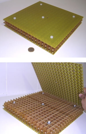
Figure 1: Photograph of the quasi-magnetostatic metamaterial lens analysed in this paper.

II Geometry of the problem

The metamaterial lens described in Ref. FreMarJel08 is composed of capacitively loaded rings (CLRs) periodically arranged in an isotropic three-dimensional lattice with the lattice constant $a=1.5$ cm. The lens features three planes of 18 by 18 CLRs interlayered with orthogonal segments providing two mutually orthogonal sets of two layers 17 by 18 CLRs each (see Fig. 1 for clarity), which makes it up to roughly 2200 CLRs. This lens can be optionally extended by an extra 3D-layer, resulting in having four $18\times 18$ layers interlaced with the two orthogonal subsystems of 3 by 17 by 18 CLRs, amounting to about 3130 elements. Overall dimensions of the (non-extended) lens are thus $27\times 27\times 3$ cm.

The CLRs themselves (Fig. 2a) are made of copper through etching metallic strips on a dielectric board. The mean radius $r_{0}$ of the CLRs is 0.49 cm ($r_{0}/a=0.33$) and the strip width $w$ is 0.22 cm ($w/a=0.15$). The CLRs are loaded with lumped non-magnetic 470 pF capacitors. The self-inductance of the CLRs, $L=\omega^{2}_{0}/C=13.5$ nH, has been obtained from the measured value of the frequency of resonance in free space, equal to 63.28 MHz ($k_{0}a=0.02$). By measurement of the quality factor of the resonator the resistance has been estimated as $R=0.0465$ Ohm, which includes the effects of both the ring and the capacitor.

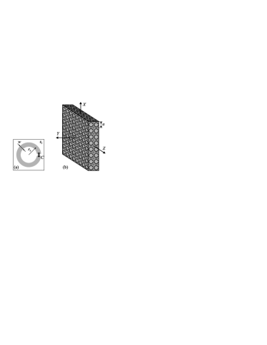
Figure 2: (a) Sketch of the CLR resonator; (b) Scheme of the lens with the corresponding coordinate system.

We reserve the standard coordinate system ($x$, $y$, $z$) for discussions on the level of geometry of one ring and their mutual interactions, as relevant for the next section. When referring the overall lens geometry, we define supplementary coordinate system ($X$, $Y$, $Z$) so that the lens geometrical centre is placed at the coordinate origin, and the $Y$ axis is perpendicular to the lens as slab (“lens axis”), while the long edges of the lens are parallel to $X$ and $Z$ axes (Fig. 2b). Note that the coordinate origin is between the rings, and thus the lens is completely symmetric with respect to the coordinate origin, all the axes and all the coordinate planes (in the analysis, we neglect minor asymmetry occurring in the real lens caused by specific assembly details, e.g. resulting from substrate thickness, as these deviations are of the same order as unavoidable production inaccuracy). For the three mutually orthogonal sets of CLRs, we will refer to as X-rings, Y-rings or Z-rings, depending on whether the rings’ normals are along $X$, $Y$ or $Z$ axes. The lens, therefore, contains 612 of either X-rings and Z-rings, and 972 Y-rings. We will also introduce a consecutive numbering of all the CLRs with a single index. The so called input and output surfaces of the lens correspond to $Y=\mp 1.5$ cm, while the theoretical source and image planes are at $Y=\mp 3.0$ cm.

III Theoretical model

For the analysis of the lens response to the external field, we consider an ideal cubic lattice of L–C circuits supporting current. With the time convention as $I\propto\exp({\mathrm{j}}\omega t)$, each of the currents is governed by equation

$$Z_{0}I_{n}=-{\mathrm{j}}\omega\Phi_{n},$$ (1)

where the self-impedance $Z_{0}=\left(R+{\mathrm{j}}\omega L+1/\left({\mathrm{j}}\omega C\right)\right)$ is determined by the resistance $R$, self-inductance $L$ and self-capacitance $C$ of the single CLR, while $\Phi_{n}$ represents the total magnetic flux through the considered ring which can be written as

$$\Phi_{n}=\Phi_{n}^{\text{ext}}+\sum\limits_{m\neq n}{\Phi_{nm}}=\Phi_{n}^{\mathrm{ext}}+\sum\limits_{m\neq n}{M_{nm}I_{m}}$$ (2)

where $\Phi_{n}^{\rm{ext}}$ is the magnetic flux from external sources and $M_{nm}$ are the mutual inductances between the rings $n$ and $m$. Combining Eq. (1) and Eq. (2) we obtain

$$\mathbf{\overline{Z}}\cdot\mathbf{I}=-{\mathrm{j}}\omega{\mathbf{\Phi}}^{\mathrm{ext}}$$ (3)

with $Z_{nn}=Z_{0}$, $Z_{nm}=\mathrm{j}\omega M_{nm}$, which is a system of linear equations for unknown currents, provided that the external sources are known.

Mutual inductance between the flat rings (which is the case under consideration) carrying the currents $I_{n}$ and $I_{m}$ uniform along the ring contour is, most generally Landau ,

$$M_{nm}=\frac{\mu}{4\pi I_{n}I_{m}}\int\limits_{S}\!\int\limits_{S^{\prime}}\frac{\mathbf{K}_{n}(\mathbf{r})\cdot\mathbf{K}_{m}(\mathbf{r^{\prime}})}{\left|\mathbf{r}-\mathbf{r^{\prime}}\right|}\>\mathrm{d}S\,\mathrm{d}S^{\prime}$$ (4)

where $\mathbf{K}$ represent surface current densities; we assume that these follow Maxwellian distribution across the strip,

$$K_{\varphi}(\rho)=\frac{2I}{w\pi\sqrt{1-\left(\dfrac{\rho-r_{0}}{w/2}\right)^{2}}},\quad\int\limits_{r_{0}-w/2}^{r_{0}+w/2}{K_{\varphi}\>\mathrm{d}\rho}=I.$$ (5)

Clearly, such integration is not ideally suited for numerical calculation. In the first approximation, mutual inductance between CLRs can be estimated with the one between linear currents (double linear integration along the equivalent ring contour), but for close CLRs this does not give a good precision.

However, a trick is that the result of surface integration according to Eq. (4) can be approximated with a good precision through an average mutual inductance between two pairs of circular currents RosaGrover . This way, each flat ring can be represented by a pair of coaxial circular currents of radii $r_{0}\pm\gamma w/2$, and the sought mutual inductance is calculated as an average between the four corresponding linear ones:

$$M_{nm}=\left(L^{++}_{nm}+L^{--}_{nm}+L^{+-}_{nm}+L^{-+}_{nm}\right)/4,$$ (6)

which essentially decreases calculation time. The value of particular parameter $\gamma$ depends on the ring geometry, but does not depend remarkably on the relative orientation and distance between the CLRs (within the limits of lens structure). For the particular parameters considered here, $\gamma\approx 0.7$ was numerically found to give a good match to the precise integration (4) (while $\gamma=1$ would correspond to the edges of the strip).

Figure 3: Geometry of the linear currents for parallel or orthogonal ring orientations, as relevant for mutual inductance calculations.

To achieve a faster calculation for the “linear” mutual inductance itself, we further note that it can be easily evaluated Landau by integrating the vector potential $\mathbf{A}$ along the current contour $l$:

$$L_{nm}=\frac{1}{I_{n}}\int\limits_{l_{m}}\mathbf{A_{\mathit{n}}}\cdot\mathbf{dl_{\mathit{m}}},$$ (7)

with vector potential itself having only $A_{\varphi}$ component (assuming that the source ring is placed at the coordinate origin with the normal along $z$ axis, see Fig. 3), which can be obtained with the help of elliptic integrals as Landau

$$A_{\varphi}=I\frac{\mu_{0}}{4\pi}\sqrt{\frac{r_{0}}{\rho}}\left(\frac{\left(2-\kappa^{2}\right)\mathcal{K}(\varkappa)-2\mathcal{E}(\varkappa)}{\varkappa}\right),$$ (8)

with

$$\varkappa=\sqrt{\frac{4r_{0}\rho}{(\rho+r_{0})^{2}+z^{2}}}$$

being the argument of complete elliptic integrals

$$\mathcal{E}=\int\limits_{0}^{\pi/2}\sqrt{1-\varkappa^{2}\sin^{2}\theta}\;\mathrm{d}\theta,\qquad\mathcal{K}=\int\limits_{0}^{\pi/2}\frac{\mathrm{d}\theta}{\sqrt{1-\varkappa^{2}\sin^{2}\theta}}.$$

Given the fact that the fast pre-defined routines for elliptic integrals are available in a number of computational platforms (e.g. Matlab^®), this effectively reduces double integration to a single one. Thus, finally, only four linear integrals like (7) are required to approximate the exact value of a double integration like (4).

IV Numerical implementation

To analyse the response of the lens to an external field source, the key step lies in solving system (3). To do so, we need to know the matrix of mutual inductances $\mathbf{\overline{M}}$. This matrix is only determined by the geometry of the rings arrangement inside the lens and can be calculated once for a given lens geometry, while the impedance matrix $\mathbf{\overline{Z}}$ can be then obtained for all frequencies as shown after (3).

For such a lens as described above, having 2196 rings, the matrix contains almost 5 million values, and filling those with a direct calculation would be rather time-consuming even with a simplified integration described in the previous section. However, obvious reciprocity ($M_{nm}=M_{mn}$) and symmetry properties of the lens allow for a great simplification of matrix filling. Indeed, the lens is symmetric with respect to $X$, $Y$ and $Z$ axes as well as to $XY$, $YZ$ and $ZX$ planes. This implies, in particular, that the mutual inductances between X-rings and Y-rings are all the same as between Z-rings and Y-rings. Furthermore, as all the rings are identical, inductance between them is only determined by their mutual orientation and spatial offsets $\Delta x$, $\Delta y$, $\Delta z$ (see Fig. 3), and for parallel rings even $\Delta x$ is equivalent to $\Delta y$. Explicitly, integration for the mutual inductances between the parallel rings is performed according to

$$L^{\text{P}}(\Delta b,\Delta z)=\int\limits_{0}^{2\pi}A_{\varphi}\frac{r_{2}(r_{2}+\Delta b\cos\alpha)}{\Delta\rho}\;\mathrm{d}\alpha,$$ (9)

$$\Delta\rho=\sqrt{r_{2}^{2}+(\Delta b)^{2}+2r_{2}\Delta b\cos\alpha},$$

$$\varkappa^{2}={\frac{4r_{1}\Delta\rho}{(\Delta\rho+r_{1})^{2}+(\Delta z)^{2}}}$$

where $\Delta b=\sqrt{(\Delta x)^{2}+(\Delta y)^{2}}$; and for the rings with orthogonal mutual orientation

$$L^{\text{O}}(\Delta x,\Delta y,\Delta z)=\int\limits_{0}^{2\pi}A_{\varphi}\frac{r_{2}\Delta y\cos\alpha}{\Delta\rho}\;\mathrm{d}\alpha,$$ (10)

$$\Delta\rho=\sqrt{(\Delta x-r_{2}\sin\alpha)^{2}+(\Delta y)^{2}},$$

$$\varkappa^{2}={\frac{4r_{1}\Delta\rho}{(\Delta\rho+r_{1})^{2}+(\Delta z-r_{2}\cos\alpha)^{2}}}.$$

In the above equations, we imply a general case that the radii of the two rings ($r_{1}$ and $r_{2}$) can be different.

Thus, a number of ring pairs within the lens share the same value of mutual inductance, so it is only necessary to calculate a full set of non-equivalent mutuals and then assign those values depending on the mutual offsets. With the particular lens considered here, there are only 1924 independent inductances for the parallel ring orientation, and 1668 for the orthogonal one, so the total number of calculations (6) is 3592 — orders of magnitude smaller than the number of matrix elements. This way, the entire matrix can be filled in a matter of seconds on an ordinary PC.

Another preliminary step is to determine the external flux $\mathbf{\Phi}^{\text{ext}}$ imposed to each ring by a given source. For a homogeneous field or a plane wave excitation, calculation is straightforward with the known coordinates of each ring:

$$\Phi_{n}^{\text{ext}}=\pi r_{0}^{2}\,\mathbf{B}_{n}\cdot\mathbf{n},$$ (11)

where $\mathbf{n}$ is a ring normal while magnetic field $\mathbf{B}_{n}$ can be evaluated at the ring centre as the field variation across the ring is negligible.

Figure 4: Frequency dependence of the real (a) and imaginary (b) parts of the impedance measured by a 3-inch coil placed at the image plane ($Y=-3$ cm).

In practice, the lens is typically used along with excitation / measuring coils employed in MRI practice. In that case, instead of calculating the field produced by a coil over each ring (which is further complicated as this field is not uniform across the ring), it is much easier to obtain the flux directly

$$\Phi_{n}^{\text{ext}}=M^{\text{c}}_{n}I^{\text{c}}$$ (12)

in terms of mutual inductance $M^{\text{c}}_{n}$ between the coil and each ring, which can be calculated with the same method as the one between the rings. Above, $I^{\text{c}}\equiv I_{\text{N+1}}$ is the total current induced in the coil by the external voltage source as well as by the lens. Imposing a given voltage $V_{\text{c}}$ to the coil with the self-impedance $Z_{\text{c}}$, we can include the coil mutual impedances into system (3), modified as

$$\mathbf{\overline{Z}}\cdot\mathbf{I}=\mathbf{V}$$ (13)

$$Z_{nn}=\begin{cases}Z_{0}\\ Z_{\text{c}}\end{cases}Z_{nm}=\begin{cases}\mathrm{j}\omega M_{nm}&\text{for}\quad 1\leqslant n\leqslant N\\ \mathrm{j}\omega M^{\text{c}}_{n}&\text{for}\quad n=N+1\end{cases}$$

with $V_{n}=V_{\text{c}}\,\delta_{n,N}$ and $N$ being the total number of rings in the lens. Clearly, additional coils, if necessary, can be included by extending the matrix system in an analogous way.

After the above procedures, it is finally possible to solve the systems (3) or (13) obtaining currents $I_{n}$ in each ring for any given excitation. With these known, it is further possible to calculate any desired response of the lens, such as magnetic field produced by the lens (using standard Biot-Savart expressions) or impedance as measured by the MRI coil,

$$Z^{\text{coil}}=\sum\limits_{n=1}^{N}\mathrm{j}\omega M^{\text{c}}_{n}\>\frac{I_{n}}{I^{\text{c}}}.$$ (14)

V Results and discussion

Armed with the above precise method, we can have a detailed look into lens features and response to various external field sources. In previous work JelMarFre09 it was concluded that the accurate model, developed for an 2D-infinite slab with the same structure and thickness as the real lens, is capable of predicting the observations made in connection to lens use in MRI practice. In a typical setup, a coil of 3 inch in diameter is placed parallel to the lens interface at the source plane, $Y=-3$ cm (that is, at a distance 1.5 cm, equal to one half of the lens thickness from the lens surface). The super-lens behaviour implies that the magnetic field produced by the coil, is then reproduced in the space behind the image plane ($Y=3$ cm), as if the coil itself were present in place of the image.

Figure 5: Axial component $H_{Y}$ of the total magnetic field observed behind the lens surface along the lens axis (1) or along the parallel line (2) slightly displaced in $X$ and $Z$ direction so that it passes through the centre of one ring (see the inset for the labels of the axes). Comparison between the two models when the lens is excited by 3-inch coil, centred with respect to the lens axis and placed at $Y=-1.5$ cm.

A straightforward example to test the developed model and to compare it with practice as well as with earlier models, is to evaluate the impedance as measured by a coil in front of the lens, depending on frequency. In the discrete model, it is given by Eq. (14), while with the continuous model (for an infinite homogeneous slab with an appropriate effective permeability BaeJelMar08 ) it can be numerically calculated as

$$Z^{\text{coil}}=-\dfrac{1}{I^{\text{c}}}\>\mathsf{Re}\int\limits_{\text{coil}}\mathbf{E}^{\text{r}}\cdot\mathbf{dl}^{\text{c}},$$ (15)

where $\mathbf{E}^{\text{r}}$ is electric field reflected by the lens. The two modelling results are compared in Fig. 4 along with the experimental data. Although there is no exact quantitative matching to the measured data, it is clear that the frequency dependence provided by the discrete model is closer to experiment than that of the continuous calculation. On the other hand, we can conclude that the latter already provides qualitatively suitable picture, predicting an overall pattern of the impedance frequency dependence.

With both the continuous model JelMarFre09 and the model developed above, it is easy to obtain the axial magnetic field $H_{Y}$ behind the lens for a given excitation. Comparison between the predictions of the two models is shown in Fig. 5. One can see that at distances smaller than about one lattice constant ($a=1.5$ cm), $H_{Y}$ is essentially inhomogeneous as the near-field of the individual rings dominates, so that the total field is quite different whether traced along the lens axis (which passes between the rings) or along a line that passes through a ring centre, while both are remarkably different from the continuous model. This is an obvious consequence of the discrete lens structure, which cannot be revealed by a homogenized model but is apparent in practice. At distances larger than approximately one lattice constant ($1.5$ cm), the field observed along the two axes converge, and are qualitatively similar to the continuous model with a fair numerical agreement (see Fig. 5).

Figure 6: Axial component $H_{Y}$ of the magnetic field observed behind the lens surface. Horizontal axis corresponds to the lens surface (parallel to $X$–$Z$ plane), while the vertical one is normal to the lens ($Y$). Only one half of the symmetrical field spatial distribution is presented; normalized magnitudes are shown in logarithmic scale between 10 (white) and 0.1 (black) A/m. Excitation with coils of different radii (0.5 cm, 1.5 cm, 3 cm and 4.5 cm), centred with respect to the lens axis and positioned at $Y=-1.5$ cm.

Another peculiarity arising from the discrete structure is related to the spatial resolution of the lens in the $X$–$Z$ plane. Evidently, a lens cannot resolve any details which are separated by distances of the order of lattice constant. To identify the actual limitation, we test the magnetic field distributions originating from using the coils of various small radii (Fig. 6). For excitations with a coil of the ring size, the entire lens is dominated by standing magnetoinductive waves SKR2b , and the field pattern does not suggest any hints for resolving the source (Fig. 6a). Indeed, practically the same field pattern is observed with a three times larger coil, two lattice constants in diameter (Fig. 6b). With a still larger coil, encompassing four lattice constants, one may argue that the pattern starts to clarify (Fig. 6c), though still it cannot be reliably used to assess the source location and size. A reasonable picture is obtained for a 4.5 cm coil radius, where the field farther than the image plane looks as expected with super-lens performance (Fig. 6d). We can therefore conclude that spatial resolution of the discrete lens can be assumed to be of the order of 5 lattice constants. This observation is in good agreement with the general concerns regarding the lattice effects in metamaterials GLS2 .

With the above examples, we clearly demonstrate that the exact model described in this paper, is suitable for a reliable description of the metamaterial lens, and makes it possible to predict specific observations which might be missed by a continuous model.

Certainly, the above methodology is not restricted to the particular lens geometry and can be perfectly used for any metamaterials designed with CLRs or SRRs, whether isotropic or anisotropic, and also arbitrarily small in size. The only limitation is that for very large number of elements, numerical evaluation on conventional computers may fail, specifically as far as allocating space for huge impedance matrices, and inverting these, is concerned. However, in metamaterial research it rarely comes to samples that large, and, on the other hand, when it comes, then there are good reasons to expect that continuous models will work sufficiently fine.

In contrary, for small metamaterials typically considered for practical use, modelling this way provides an invaluable insight into their properties and leads to reliable predictions.

- (1) Solymar, L., and Shamonina, E., ‘Waves in Metamaterials’ (Oxford University Press, 2009).
- (2) Marqués, R., Martín, F., and Sorolla, M., ‘Metamaterials with negative parameters’ (Wiley, 2008).
- (3) Lapine M., and Tretyakov, S., ‘Contemporary notes on metamaterials’, IET Microwaves Antennas & Propagation, 2007, 1, pp. 3–11.
- (4) Sihvola, A., ‘Metamaterials in electromagnetics’, Metamaterials, 2007, 1, pp. 2–11.
- (5) Pendry, J.B.: ‘Negative refraction makes a perfect lens’, Phys. Rev. Lett., 2000, 85, pp. 3966–3969.
- (6) Shamonina, E., Kalinin, V.A., Ringhofer, K.H., and Solymar, L.: ‘Imaging, compression and Poynting vector streamlines for negative permittivity materials’, Electron. Lett., 2001, 37 (20), pp. 1243–1244.
- (7) Maslovski, S., Tretyakov, S., and Alitalo, P.: ‘Near-field enhancement and imaging in double planar polariton-resonant structures’, J. Appl. Phys., 2004, 96 (3), pp. 1293–1300.
- (8) Mesa, F., Freire, M.J., Marqués, R., and Baena, J.D.: ‘Three-dimensional superresolution in metamaterial slab lenses: Experiment and theory’, Phys. Rev. B, 2005, 72, 235117.
- (9) Freire, M.J., and Marqués, R.: ‘Planar magnetoinductive lens for three-dimensional subwavelength imaging’, Appl. Phys. Lett., 2005, 86, 182505.
- (10) Freire, M. J., R. Marqués, and L. Jelinek, “Experimental demonstration of a metamaterial lens for magnetic resonance imaging”, Appl. Phys. Lett., 2008, 93, 231108.
- (11) Grbic, A., and Eleftheriades, G.V.: ‘An isotropic three-dimensional negative-refractive-index transmission-line metamaterial’, J. Appl. Phys., 2005, 98, 043106.
- (12) Alitalo, P., and Tretyakov, S., ‘Subwavelength resolution with three-dimensional isotropic transmission-line lenses’, Metamaterials, 2007, 1, pp. 81–88.
- (13) Solymar, L., Zhuromskyy, O., Sydoruk, O., Shamonina, E., Young I.R. and Syms R.R.A.: ‘Rotational resonance of magnetoinductive waves: basic concept and application to nuclear magnetic resonance’, J. Appl. Phys., 2006, 99, 123908.
- (14) Syms, R.R.A., Solymar, L., and Young, I.R., ‘Three-frequency parametric amplification in magneto-inductive ring resonators’ Metamaterials, 2007, 2, pp. 122–134.
- (15) Syms, R.R.A., Young, I.R., and Solymar, L., ‘Flexible magnetoinductive ring resonators: Design for invariant nearest neighbour coupling’ Metamaterials, 2010, 4 (in press).
- (16) Wiltshire, M.C.K., Hajnal, J.V., Pendry, J.B., Edwards, D.J., and Stevens, C.J.: ‘Metamaterial endoscope for magnetic field transfer: Near field imaging with magnetic wires’, Opt. Express, 2003, 11, pp. 709–715.
- (17) Ikonen, P., Belov, P.A., Simovski, C.R., and Maslovski, S.I.: ‘Experimental demonstration of subwavelength field channeling at microwave frequencies using a capacitively loaded wire medium’, Phys. Rev. B, 2006, 73, 073102.
- (18) Radu, X., Garray, D., Craeye, C., ‘Toward a wire medium endoscope for MRI imaging’, Metamaterials, 2009, 3, pp. 90–99.
- (19) Agranovich, V. M., and Gartstein, Yu. N., ‘Electrodynamics of metamaterials and the Landau-Lifshitz approach to the magnetic permeability’, Metamaterials, 2009, 3, pp. 1–9.
- (20) Simovski, C., ‘Analytical modelling of double-negative composites’ Metamaterials, 2008, 2, pp. 169–185.
- (21) Silveirinha, M. G., ‘Metamaterial homogenization approach with application to the characterization of microstructured composites with negative parameters’, Phys. Rev. B, 2007, 75, 115104.
- (22) Gorkunov, M., Lapine, M., Shamonina, E., and Ringhofer, K.H.: ‘Effective magnetic properties of a composite material with circular conductive elements’, Eur. Phys. J. B, 2002, 28, pp. 263–269.
- (23) Baena, J. D., L. Jelinek, R. Marqués, and M. Silveirinha, ‘Unified homogenization theory for magnetoinductive and electromagnetic waves in split-ring metamaterials’, Phys. Rev. A, 2008, 78, 013842.
- (24) Jelinek L., R. Marqués, and M. J. Freire, ‘Accurate modelling of split ring metamaterial lenses for magnetic resonance imaging applications’, J. Appl. Phys., 2009, 105, 024907.
- (25) Landau, L.D., and Lifschitz, E.M.: ‘Electrodynamics of Continuous Media’ (Pergamon Press, Oxford, 1984).
- (26) Rosa, E. B., and Grover, F. W., ‘Formulas and tables for the calculation of mutual and self induction’, Bulletin of the Bureau of Standards, 1916, 8 I (Washington, 1948).
- (27) Shamonina, E., Kalinin, V.A., Ringhofer, K.H., and Solymar, L.: ‘Magnetoinductive waves in one, two, and three dimensions’, J. Appl. Phys., 2002, 92, pp. 6252–6261.