Fit;o) - A Mössbauer spectrum fitting program

Abstract

Fit;o) is a Mössbauer fitting and analysis program written in Borland Delphi. It has a complete graphical user interface that allows all actions to be carried out via mouse clicks or key shortcut operations in a WYSIWYG fashion. The program does not perform complete transmission integrals, and will therefore not be suited for a complete analysis of all types of Mössbauer spectra and e.g. low temperature spectra of ferrous silicates. Instead, the program is intended for application on complex spectra resulting from typical mineral samples, in which many phases and different crystallite sizes are often present at the same time. The program provides the opportunity to fit the spectra with Gaussian, Lorentzian, Split-Lorentzian, Pseudo-Voigt, Pseudo-Lorentz and Pearson-VII line profiles for individual components of the spectra. This feature is particularly useful when the sample contains components, that are affected by effects of either relaxation or interaction among particles. Fitted spectra may be printed, fits saved, data files exported for graph creation in other programs, and analysis tables and reports may be exported as plain text or LaTeX files. With Fit;o) even an inexperienced user will soon be able to analyze and fit relatively complex Mössbauer spectra of mineralogical samples quickly without programming knowledge.

PACS: 33.45.+x , 82.80.Ej , 61.18.Fs

, ,

1 Introduction

During work with analysis of Mössbauer spectra we found that existing analysis software packages however competent (i.e. Mfit [1], Recoil [2], MacFit [3], MossWinn[4]) could not fulfill our needs of being simple and yet very flexible. For fitting of spectra with many components, as is typical for samples with complex mineral assemblies, advanced programs are in many cases too detailed to be really useful.

We therefore developed this program package which attempts to mitigate these issues, and thus provides a powerful tool for rapid fitting of complex Mössbauer spectra.

The program has been downloaded around 100 times in several versions, and an estimate of regular users is around 20. The program package has been used in the preparation of several articles or talks [5, 6, 7, 8, 9].

2 Program summary

Fit;o) is a program for fitting and analyzing transmission and scattering geometry ⁵⁷Fe Mössbauer spectra of metals, alloys and mixtures of ferric oxides, oxyhydrates and silicates. The program can be expanded to handle other Mössbauer isotopes as well. It has a complete graphical user interface, which allows all actions to be performed via mouse clicks or key shortcuts. The program accepts currently both particular plain text files (.exp-files, see [10, 11] for a definition) and comma-separated files e.g. counts vs. velocity (velocity;counts) as data input. It is the intention to release the source code under an open license.

Mössbauer spectra can be fitted using singlets, doublets and sextets (all with a selection of line profiles of which Lorentzian is default) and the fit model can be saved for later reloading for example for further refinement of the fit. Fitted and unfitted spectra can be saved as reports and saved as both plain text and in customizable LaTeXformat, and spectra can be printed with a fit report.

The program contains a precompiled list of Mössbauer data of many common iron compounds with an option for the user to edit or add new compounds.

Calibration data for Mössbauer experimental setups can be extracted from calibration spectra, and saved in separate calibration .cal-files (see [10, 11] for a description).

The settings window contains a wide range of customizable settings through which the user may customize the appearance and behavior of the program. Backwards compatibility is ensured, as file formats are kept unchanged and user-changed files are not overwritten.

The web update option provides an easy and automated way to keep the software updated with the latest program version.

The program does not perform complete transmission integrals, and will therefore not be suited for a complete analysis of all types of Mössbauer spectra. Also the fitting does not use the complete spin-Hamiltonian (but approximations) so for example magnetic (low-temperature) spectra of silicates cannot be analyzed by the programme.

Some of Fit;o)’s main features are:

• Microsoft Windows 2000/XP compatible.

• Easy to install, no external dependencies, and safe uninstallation/removal.

• Complete point-and-click graphical user interface.

• Easy saving and loading of fit models.

• Most program parameters as customizable.

• Working with several spectra (MDI) at a time is possible.

• Created with object-oriented programming.

3 Description

3.1 Prerequisites

As noted in the introduction, execution of Fit;o) requires an updated Microsoft Windows 2000, Microsoft Windows XP operating system. A screen resolution of a least 1024x768 with a 16 bit color depth is recommended.

3.2 Installation and execution

The program is available at http://hjollum.com/jari/zzbug/fit/. After installation and execution the main options are:

• Open the selected type spectrum by selecting an appropriate icon in File menu.

• To open a file in text mode, use the Open text file option and to view the application log, use the Open log option.

A more detailed description of the program interface can be found in the manual [10] or the web site [11].

3.3 The layout of the graphical user interface

After the first execution of the program the user is presented to the graphical user interface shown in figure 1. The main window of Fit;o) is divided into five areas (listed from top down), the menu bar, the tool bar, the work area, the window panel and the status panel.

3.4 Fitting

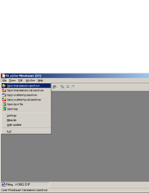
Figure 1: Opening a spectrum file.

When choosing to open a spectrum for fitting, the open spectrum form (figure 2) appears, in which the spectrum to be loaded is chosen. After choosing a spectrum the fit form (figure 3) is opened and the spectrum is loaded.

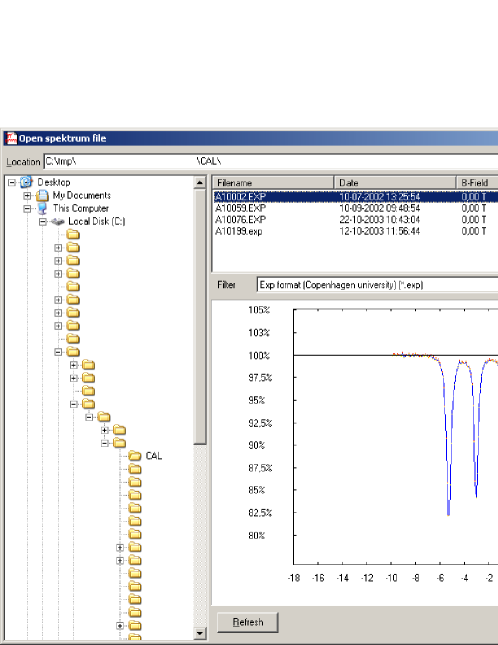
Figure 2: Choosing the spectrum to open.

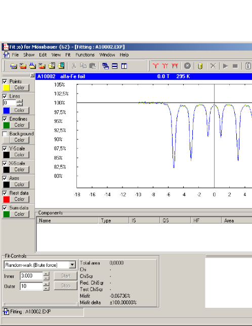
Figure 3: The fit form with a loaded spectrum.

As fitting components, it is possible to insert either simple (fundamental) components (singlets, doublets, sextets), or to insert predefined mineral components.

Simple components are inserted by clicking one of the spectrum icons in the toolbar, and then marking, position, intensity and width of the components on the graph. The parameter that the user is expected to mark is indicated at the cursor.

Predefined (but editable) mineral components are inserted by clicking the cylinder icon in the toolbar, and choosing the mineral. After choosing, one has to mark the intensity of the component on the graph using the mouse cursor.

Figure 4: The fit form with an inserted component.

The fitting algorithm is chosen in the Fit Controls combobox in the lower left corner of the form. The fitting process is started and aborted by using the adjacent start and stop.

3.5 Calibration

Fitting components are inserted by clicking the button in the toolbar with the sextet icon (see figure 5).

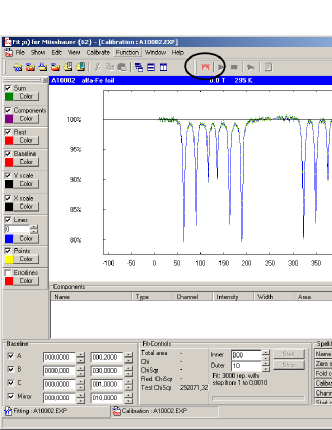
Figure 5: The calibration form before inserting the calibration fit components. The insert button is marked.

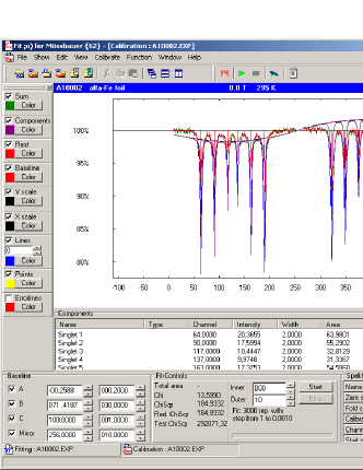
Figure 6: The calibration form after insertion of the calibration fit components.

When the components have been inserted, either a single fitting run or a series of repetitive fitting runs can be started, through the start icons. The result can be saved and exported by clicking the ’notepad’ icon.

3.6 Minerals

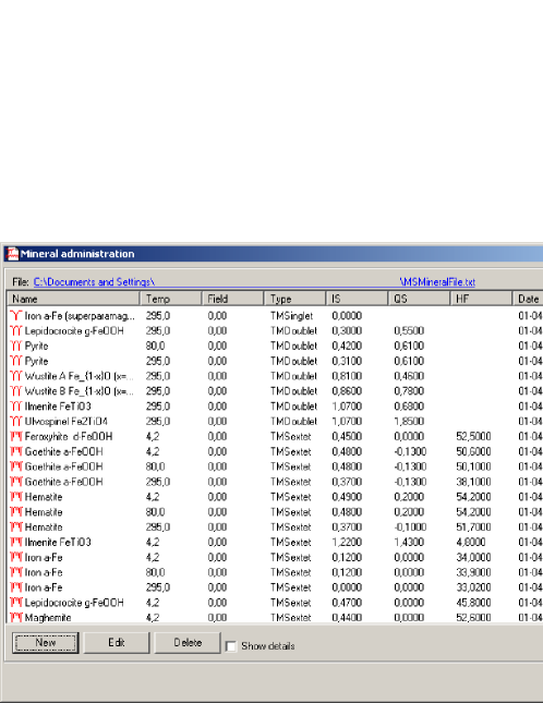
Figure 7: The minerals administration window.

The program contains a list of common and well-known minerals (figure 7), which can be used for as starting point fitting. The mineral data are from [12]. It is possible to edit the listed minerals and save these modifications, and to enter new minerals. This can be done either through the New, Edit or Delete options, or by editing the minerals file manually. The name and location of the minerals file is displayed in top of the window.

4 Project planning

In the following we discuss the properties of the program as used for analysis of a transmission/absorption spectrum. However, the discussion is completely valid also for scattering/emission spectroscopy, since there will be only few details differentiating these.

4.1 Line shapes

Ideally each Mössbauer absorption line has a Lorentzian line shape, (see table 1). However, there are physical effects that might disrupt or distort the ideal case. For these cases other line shapes are necessary.

In practice most absorbtion lines are Lorentzians, which may be sligthly smeared by a Gaussian due to for instance temperature fluctuations, leading to the Voigt line shape. The Voigt line shape is a convolution of a Lorentzian and a Gaussian and can be expressed as [13]

$$L_{Voigt}(v)=\int^{\infty}_{-\infty}L_{Gau}(v^{\prime})L_{Lor}(v-v^{\prime})dv^{\prime}.$$ (1)

However, this can not be solved analytically, and therefore several approximations to this profile exist. We have implemented three of these: Pseudo-Voigt, Pseudo-Lorentz and Pearson-VII, which are listed in table 1. Especially the Pearson-VII line shape is difficult to implement, since it involves the implementation of the Gamma function [14], which was implemented using Stirlings approximation [15]

$$\Gamma_{Stirling}(z)\cong\sqrt{\frac{2\pi}{z}}\Bigg{(}\frac{z}{e}\sqrt{z\sinh\frac{1}{z}+\frac{1}{810z^{6}}}\Bigg{)}^{z},$$ (2)

which is accurate to a least 5 digits for z>1.

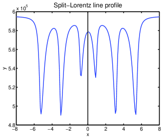
Figure 8: An example of a spectrum with Split-Lorentzian line profiles. The outer slope of an absorption line is defined as the slope farthest from the center of the component. This of course only applies to doublets and sextets.

The Split-Lorentzian (see figure 8) line shape is commonly used for samples in which small-particle effects or interactions distort the line shapes in such a way that the outer slope is steeper than the inner slope. The Split-Lorentzian line shape is made up of the outer side using one Lorentzian line shape, and the inner side using another shape. The amplitude and center of the two line shapes are kept equal, but the widths vary. The relationship between the widths is usually controlled by defining a width parameter and an asymmetry parameter. The asymmetry parameter is usually known as $b$.

When using the Split-Lorentzian line shape in doublets and sextet (see section 4.2) the line shapes are mirrored with respect to the center of the component, and the left side of a line shape is identical to the right side of its mirrored twin.

The line shapes implemented for the Mössbauer analysis and the properties of these are presented in table 1.

Name	Formula	Area	Additional
			parameters
Lorentzian	$L_{Lor}(v)=I_{0}\big{(}1+\big{(}\frac{2(v-v_{0})}{W}\big{)}^{2}\big{)}^{-1}$	$A_{Lor}=\frac{I_{0}W\pi}{2}$	-
Gaussian	$L_{Gau}(v)=I_{0}\exp\big{(}-\big{(}\frac{2(v-v_{0})}{W}\big{)}^{2}\big{)}$	$A_{Gau}=\frac{I_{0}W\sqrt{\pi}}{2}$	-
Split-Lorentzian	$L_{S-L}(v)=\bigg{\{}\begin{array}[]{cc}L_{Lor}(W_{1})&,\quad v<v_{0}\\ L_{Lor}(W_{2})&,\quad v\geq v_{0}\end{array}$	$A_{S-L}=\frac{1}{2}\sum_{i=1}^{2}A_{Lor}(W_{i})$	$\begin{array}[]{c}b\equiv\frac{W_{1}}{W_{2}}-1\\ W_{1}\geq W_{2}\end{array}$
Pseudo-Voigt	$L_{Pseu}(v)=\eta\cdot L_{Lor}+(1-\eta)\cdot L_{Gau}$	$A_{Pseu}=\eta\cdot A_{Lor}+(1-\eta)\cdot A_{Gau}$	$\eta\in[0;1]$
Pseudo-Lorentz	$L_{PLor}(v)=I_{0}\big{(}1+\big{|}\frac{2(v-v_{0})}{W}\big{|}^{2+\alpha}\big{)}^{-1}$	$A_{PLor}=\frac{I_{0}W\pi}{2}\frac{2sin(\frac{\pi}{2+\alpha})}{2+\alpha}$	$\begin{array}[]{c}\alpha\in[0;1.45]\\ \alpha=0\quad Lorentz\end{array}$
Pearson-VII	$L_{PVII}(v)=I_{0}\big{(}1+\big{(}\frac{2(v-v_{0})}{W}\big{)}^{2}\frac{1}{m}\big{)}^{-m}$	$A_{PVII}=\frac{I_{0}W\sqrt{m\pi}}{2}\frac{\Gamma(m-\frac{1}{2})}{\Gamma(m}$	$\begin{array}[]{c}m\geq 1\\ m=1\quad Lorentz\\ m\rightarrow\infty\quad Gauss\end{array}$

Table 1: Line shapes used for Mössbauer analysis. Reproduced from [16].

4.2 Fit components

The three fundamental Mössbauer fitting components are the singlet, the doublet and the sextet with 1, 2 and 6 absorption lines, respectively. All of these components are characterized by their isomer shift (IS).

The splitting of the doublet depend on the quadrupole interaction, and is in the doublet quadrupole splitting (QS).

The singlet, doublet and the sextet have furthermore the line shape a parameter ($b$, $\eta$, $\alpha$ and $m$ in table 1) in common. The Split-Lorentzian, Pseudo-Voigt, Pseudo-Lorentz and Pearson-VII line shapes use this property.

The magnetic Zeeman interaction, the magnetic hyperfine field (HF), is only used in the sextet, and needs only to be implemented in the sextet. For sextets this software - presently - can handle only spectra in which the magnetic Zeeman interaction is dominant, so that the quadrupole interaction can be treated as a small perturbation on the magnetic interaction. In the case of the sextet QS indicates the quadrupole shift in contrast to the doublet quadrupole split.

However, since the properties HF, and QS, are the only properties which do not apply to all components, we have provided an interface to them in all components, but disabled them where they are not needed. As mentioned, we do not use the complete spin-Hamiltonian for calculations of the line positions in the, but rather approximate expressions, which however, have been quite sufficient in most all cases.

The singlet consists of a single line, and the position of the single line is the same as the isomer shift. The expression for the singlet is given by

$$y_{i}=L(v_{i}-v_{0}),$$ (3)

where $L$ is the line shape function providing the value of $y_{i}$ as a function of $v_{i}$, and $v_{0}$ is the value of the isomer shift.

The doublet consists of two lines, and the centers of the lines are placed at a distance of QS apart, around the isomer shift. The expression for the doublet is given by

$$y_{i}=L(v_{i}-v_{0}-\frac{v_{0}}{2})+L(v_{i}-v_{0}+\frac{v_{QS}}{2}),$$ (4)

where $v_{QS}$ is the value of the quadrupole splitting.

The sextet consists of six lines, and the centers of the lines are placed at positions dictated by the isomer shift, quadrupole shift and hyperfine field.

The expression for the sextet is given by

$$y_{i}=\sum_{i=1}^{6}L(v_{i}-v_{0}+(-1)^{(1+\delta_{2345})}\frac{v_{QS}}{2}+(-1)^{(1+\delta_{456})}k_{q,w}\cdot B_{HF}),$$ (5)

where $\delta_{mnkl}$ is a delta function, which is 1 when $i$ has one of its values. $k_{q,w}$ is a Mössbauer proportionality factor, composed of several physical constants. The three values that apply are $k_{1,6}$, $k_{2,5}$, $k_{3,4}$ for the paired lines. $B_{HF}$ is the hyperfine field. The $k_{i,j}$ values are calculated from the general expression for the sextet energy levels, which is given by

$$E_{m}=-g\beta_{n}mB,$$ (6)

where $g$ is the Landé factor, $\beta_{n}$ is the nuclear magneton, and $m$ is the m-quantum number. The energy splitting is calculated by

$$|\Delta E_{(i,j)}|=|\Delta E_{i}|+|\Delta E_{j}|=2|\Delta E_{i}|,$$ (7)

where $(i,j)=(1,6),(2,5),(3,4)$. Applied to the line pairs (1,6), (2,5), (3,4) then energy splitting is calculated from

$$|\Delta E_{(i,j)}| = -2(\beta_{n}B(g_{e}\frac{3}{2}-g_{g}\frac{1}{2}))=\beta_{n}B\cdot g_{ij},$$ (8)

where $g_{g}=0.181208$ and $g_{e}=-0.10355$ are the g-factors for the ground state and the excited state respectively, values from [12], and the $g_{ij}$ factors,

$$g_{16} = -2(g_{e}\frac{3}{2}-g_{g}\frac{1}{2})=0.491858,$$ (9)

$$g_{25} = -2(g_{e}\frac{1}{2}-g_{g}\frac{1}{2})=0.284758,$$ (10)

$$g_{34} = -2(g_{e}\frac{-1}{2}-g_{g}\frac{1}{2})=0.077658,$$ (11)

are g-factors extracted from the g-factor for the excited and ground state and $E_{0}$ is the transition energy from $I=\frac{3}{2}$ to $I=\frac{1}{2}$ for ⁵⁷Fe Mössbauer spectroscopy.

The actual calculation being performed is

$$v_{HF}=g_{ij}\beta_{n}B_{HF}\cdot\frac{c}{2E_{0}},$$ (13)

using unit conversion this becomes

$$v_{HF} = g_{ij}B_{HF}\frac{\beta_{n}\cdot c\cdot k}{2E_{0}e}$$ (14)

$$= g_{ij}B_{HF}\frac{5.0505\cdot 10^{-27}\,{\rm J/T}\cdot 3.0\,\cdot 10^{11}\,{\rm mm/s}}{2\cdot 14.41\,{\rm keV}\cdot 1.6022\cdot 10^{-19}{\rm J/eV}}$$ (15)

$$= g_{ij}B_{HF}\cdot 0.32794\,{\rm mm/sT},$$ (16)

where $e$ is the elementary charge. Now the $k_{q,w}$’s can be calculated as

$$k_{1,6} = 1.61299\cdot 10^{-1}\,{\rm mm/sT},$$ (17)

$$k_{2,5} = 9.33835\cdot 10^{-2}\,{\rm mm/sT},$$ (18)

$$k_{3,4} = 2.54672\cdot 10^{-2}\,{\rm mm/sT}.$$ (19)

4.3 Fitting spectra

The program will analyze Mössbauer spectra by fitting a model set by the user, and it will report the result of the fit.

Before any analysis can commence, a background level has to be established/calculated. The background level is calculated as the mean of the value of the outermost 8 channels on each side of the spectrum. Transmission spectra contain absorption lines, which have fewer counts than the background level. The expression for components provided above has to be subtracted from the background to produce a model data series.

The program can also be used for analysis of reflection spectra. Reflection spectra also contain a background level, to which the reflection lines are added. To produce a fitting model, the fitting components are added to the background level.

4.4 Calibration spectra

The program derives the calibration parameters of the spectrometer from automatic analysis of calibration spectra. The found calibration parameters are then used in the analysis of spectra obtained under circumstances identical to those of the calibration spectrum. In this program version (1.0.0.63) only calibration of linear velocity profiles are implemented. We are well aware that sinusoidal velocity profiles are common in the Mössbauer community, and a later version may be adapted for spectra obtained in the mode.

Contrary to a normal spectrum for Mössbauer analysis, a calibration spectrum is analyzed unfolded with the channel numbers used as reference.

The calibration spectrum usually consists of the spectrum of a thin iron ($\alpha$-Fe) foil (12.5 $\mu$m) at 295 K. But other calibration materials can also be used, such as stainless steel and other well characterized iron compounds.

The unfolded calibration spectrum consists of a background level, and 12 absorption lines on the background level figure 5. The calibration is used for finding 3 unknown parameters of the experimental setup, and to provide information on any imperfections of the source/drive system i.e. increased line widths, nonlinearity etc. The three unknown parameters are listed below:

The folding channel

is the channel (integer) around which the data channels are folded. Operationally (for historic reasons and backwards compatibility) it is defined as the channel number, which is added to channel number 1, e.g. it is the double of the actual folding channel. In a 512 channel setup, it has typically a value of 510-514. It is found by calculating the mean of positions of the lines (1,12), (2,11), etc.

The zero velocity channel

is defined as the detector channel position (decimal, 5 digits), of the symmetry center of the 295 K spectrum of a thin foil of $\alpha$-Fe. It is found in each of the spectrum halves separately. It is found by locating the mean center of the lines (1,6), (2,5) and (3,4) pairwise, and correspondingly for the second half of the spectrum, and then finding the common center.

The calibration constant

is the link between the channel number and the source velocity. It is found as the mean value of the known hyperfine field of the absorber material ($B_{HF}=33.02$ T for $\alpha$-Fe at 295 K) divided by the distances between the transition pairs, $(i,j)={(1,6),(2,5),(3,4)}$, and scaled by the Mössbauer constants (17). The exact formula is

$$c_{cal}=\frac{1}{6}\sum\frac{g_{ij}\beta_{n}B_{HF}}{E_{0}\cdot c}\bigg{(}\frac{1}{P_{j}-P_{i}}+\frac{1}{P_{j+6}-P_{i+6}}\bigg{)},$$ (20)

where $P_{i}$ is the channel position of the i’th absorption line.

The background line has a shape that is dependent on the mode of operation of the spectrometer (e.g. frequency and velocity range) and geometry of the experimental setup. The radioactive source is placed inside a collimator, and since the source is oscillating with near constant acceleration, the solid angle seen by the source will vary as a function of position. The radiation detected is proportional to the angular area. The baseline shape is approx. that of two parabolas in succession with positive and negative $a$ values:

$$A = +a\cdot(v-c_{M})^{2}-b(v-c_{M})+c,\quad 1\leq v\leq c_{M},$$ (21)

$$A = -a\cdot(v-c_{M})^{2}-b(v-c_{M})+c,\quad c_{M}\leq v\leq N,$$ (22)

where $A$ is the angular area, $c_{M}$ is the mirror channel, $v$ is the channel number, $N$ is the number of channels, and $a$, $b$ and $c$ are the parabola parameters.

Besides the above calculations, the calibration is able to find the 12 absorption lines (⁵⁷Fe), and fit these and the baseline to find the calibration constants.

As the equipments available during the development only used a linear velocity drives, only this case has been implemented in the program, but this is easily expanded, when the apparatus data are available.

5 The program structure

The program is built entirely on object oriented technology (OOT). There are several advantages in using OOT:

• Inheritance makes it easy to create a child class, which inherits most of its properties and methods from its ancestor, but introduces some new, or changes the internal behavior in some areas.

• Isolation makes it easy to correct errors or undesirable behavior, without affecting other parts of the program, thereby minimizing program errors. Furthermore it makes it easy to extend functionality.

There are also disadvantages in choosing OOT:

• Processing speed will in most cases be lower than that of a procedural program since the overhead will be larger, and the amounts of data manipulated in most cases will be larger.

• The implementation process will take longer and the source code will be larger, since similar behavior may have to be implemented several times in order to avoid code shared between classes.

The program was implemented using Borland Delphi 5, 6 and 7, and should be executed on a PC running Microsoft Windows 2000 or Microsoft Windows XP. During implementation the built-in classes of Delphi have been used as programming base. For increased flexibility the program is designed to be a multiple document interface (MDI) program, meaning that it would be possible to work with several ’documents’ (spectra) simultaneously.

5.1 The fitting form

The Mössbauer fitting form is implemented as the class TdfmFitForm (see figure 9). It is the graphic user interface, through which the user makes input to and receives output from the spectrum analysis. It contains two very important classes TGraph and TFitGraph.

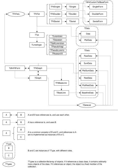
Figure 9: The logical/workflow diagram of the TdfmFitForm class, used for fitting Mössbauer spectra. The upper part is the logical/workflow diagram, and the symbol explanations are shown in the lower part.

After the FitForm has been created and initialized, it loads a data-file (which the user has chosen), and calculates the Mössbauer spectrum background level. The spectrum is folded during loading.

Whenever a change has been made to one of the fitting components, or a new fitting component has been inserted, several calculations have to be performed:

• The sum data, SumData, which contains the sum of the fitting components is calculated as

  $$S_{i}=\sum_{j=1}^{N_{tet^{\prime}s}}T_{j,i},$$ (23)

  where $S_{i}$ is the sum at the i’th point, $T_{j,i}$ is the value of the j’th fit component (singlet, doublet, sextet), at the i’th point.

• The rest data, RestData, which contains the difference between the spectrum data and the sum is calculated as

  $$R_{i} = D_{i}-(B_{i}-S_{i})=D_{i}-M_{i}\quad{\rm for\ transmission\ spectra,}$$ (24)

  $$R_{i} = D_{i}-(B_{i}+S_{i})=D_{i}-M_{i}\quad{\rm for\ scattering\ spectra,}$$ (25)

  where $R_{i}$ is the rest at the i’th point, $D_{i}$ is the i’th data point of the spectrum data, $B_{i}$ is the i’th point in the baseline and $M_{i}$ is the model data at the i’th point.

• The $\chi^{2}$, ChiSqr, and $\tilde{\chi^{2}}$ which are indicators for difference between the model and the data, and used for fitting, is calculated. The misfit is also given as an output parameter. It can be summarized mathematically to

  $$\chi^{2}=\frac{1}{n_{valid}}\sum_{i=1}^{n_{valid}}\frac{R_{i}^{2}}{D_{i}}=\frac{1}{n_{valid}}\sum_{i=1}^{n_{valid}}\frac{(D_{i}-M_{i})^{2}}{E_{i}^{2}},$$ (26)

  since $E_{i}=\sqrt{D_{i}}$ and $n_{valid}$ is the number of valid channels in the spectrum. Furthermore we calculate the reduced chi-squared $\tilde{\chi}^{2}$ by

  $$\tilde{\chi}^{2}=\frac{1}{n_{valid}-n_{free}}\sum_{i=1}^{n_{valid}}\frac{R_{i}^{2}}{D_{i}},$$ (27)

  where $n_{free}$ is the number of free fit parameters. As a goodness of fit parameter we use the misfit $m$ [17] defined by

  $$m=\frac{n(\chi^{2}-1)}{\sum_{i=1}^{n_{valid}}\frac{(B_{i}-D_{i})^{2}}{D_{i}}}.$$ (28)

Two fitting algorithms, random walk [16] and amoebe [18], have been implemented in the fitting form. First we will go through the random walk algorithm.

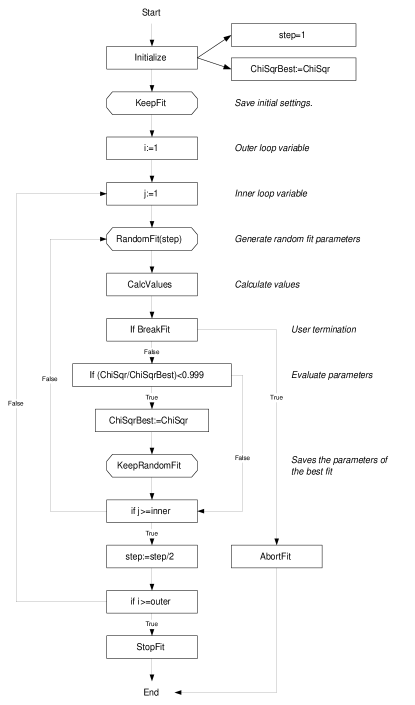
Figure 10: A graphical illustration of the RandomFit fitting algorithm. The steps marked with octagonal boxes indicate that this step iterates through all TFitTet’s in the fit.

The random walk algorithm is a variant of the "simulated annealing"-algorithm used in many areas of physics. It differs however, in that the tunneling possibility has been eliminated. The RandomFit algorithm is presented graphically in figure 10. The algorithm is based on two loops, the outer and the inner. The core of the algorithm is thus run

$$N=n_{outer}\cdot n_{inner}$$ (29)

times. The algorithm starts with setting the variable step to 1. Each time the outer loop is traversed once, step is set to one half of its previous value. The philosophy is to find the hitherto best fit for each time the outer loop has been traversed, and thereafter to narrow the interval in which the parameters are allowed to vary, before traversing to the outer loop again.

The algorithm is based on the assumption that the best fit after $n_{inner}$ guesses, lies in the vicinity of the best fit. The fitting parameters all have an interval to which they are restricted during fitting. Using the result of the sum

$$\sum_{i=0}^{\infty}2^{-i}=2,$$ (30)

this can be maintained/fulfilled. If $\Delta$ is the fitting variation interval of a fitting parameter, the following formula

$$\sum_{i=0}^{n_{outer}-1}\Delta\cdot 2^{-i}<2\cdot\Delta$$ (31)

provides a way to implement our version of the random walk algorithm without violating the restrictions:

$$\sum_{i=0}^{n_{outer}-1}1/2\cdot\Delta\cdot 2^{-i}<1/2\cdot 2\cdot\Delta=\Delta.$$ (32)

Before the first traversation of the inner loop, the variation intervals are therefore set to half of the original, corresponding to the formula above. This guarantees that the fit parameters are kept within the allowed fit interval.

The amoebe algorithm [18] works in many areas much like the random-walk algorithm. It has an outer loop, which repeats $n_{outer}$ times, or until the improvements are no longer significant. The inner loop basically works same way as in random walk.

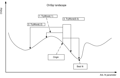
Figure 11: A graphical illustration of the preprogrammed steps in the amoebe fitting algorithm.

Besides the evaluation of the improvements mentioned, the difference between the random walk and amoebe is that after the best fit has been found using the inner loop, some preprogrammed variations of the best fit are tried. For all paramters the following is tried individually: Try to the fit parameter value in the opposite direction, with the same amount. If this gives a better fit, it tries to shift the parameter value a step further in the same direction, to see if it should give an even better fit. This tests if the point of origin was a local maximum, and if the fit has found the worst local minimum. If so, the algorithms tries if a further step in the same direction gives a better fit.

If the opposite step did not yield a better result, the algorithm tests to see if it has stepped too far to find the currently best fit, and tries to see if there is a better point halfway between the origin and the currently best fit. If all of these attempt do not result in a better fit the step variable is divided by 2, and the content of the outer loop is traversed again. If a better fit is found step is not changed. The preprogrammed steps are illustrated in figure 11.

The outer loop will terminate when it has been traversed 20 times, terminated by the user or when the rtol variable is larger than the ftol. ftol is a measure of the minimum relative improvement required, for improvements to be considered significant. rtol is a measure of the improvement of the best fit compared to the worst fit in the current traversation of outer loop. rtol is calculated from:

$$r_{tol}=2\frac{|\chi^{2}_{worst}-\chi^{2}_{best}|}{|\chi^{2}_{worst}|+|\chi^{2}_{best}|}.$$ (33)

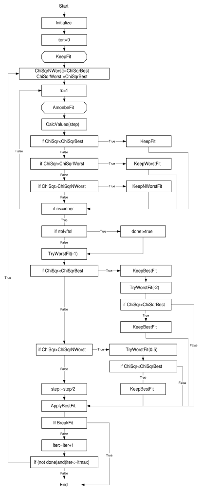
Figure 12: A graphical illustration of the AmoebeFit fitting algorithm. The steps marked with octagonal boxes indicate that this step iterates through all TFitTet’s in the fit.

The source code is presented graphically in figure 12.

5.2 The calibration form

Figure 13: The logical/workflow diagram of the TdfmCalForm class, used for fitting Mössbauer spectra. The upper part is the logical/workflow diagram, and the symbol explanations are shown in the lower part.

The Mössbauer calibration form is the graphic user interface, through which the user makes input to and receives output from the calibration process. Generally it resembles the fitting form in many points, and the description of common features will not be repeated. The data files are, however, loaded unfolded.

Whenever a change has been made to one of the fitting parameters, the same calculations as in the fitting form have to be performed. SumData, PlotSumData, RestData and PlotRestData, are calculated in the same way. The only difference with regards to the fitting form is the variable baseline in the calibrations form, which has to be taken into account.

Before the calibration process can commence, the fitting components have to be inserted, and the baseline parameters defined. The baseline is initially fixed, but is allowed to vary during the calibration. The 12 components are inserted at the 12 local extrema with the largest ’magnitude’.

The local minima are found by traversing through the data points of the data, and for each data point it checks whether the current point is a local extremum by comparing it to its neighboring points. If the point is a local extremum the magnitude is calculated as

$$M_{pivot}=\frac{y_{i+2}+y_{i+1}+y_{i-1}+y_{i-2}}{4}-y_{i},$$ (34)

where $y_{i}$ is the i’th point. After finding the all local extrema, the list of extrema is sorted, so the local extrema with the largest magnitude are placed first in the list, and the predefined number of largest local extrema are returned, and used for inserting the fitting components.

The random walk in the calibration form is very similar to that of the fitting form. The only difference lies in that the inner loop fits the components parameters when the inner loop counter j is even and the baseline parameters when it is odd. This is done since experiments during programming shows that this improves the intelligence and speed of the calibration procedure.

6 Conclusion

We have presented the functionality and the basic principles behind the Fit;o) program. We believe that by the program we have made available a valuable tool for general simple Mössbauer analysis of complex samples.

7 Acknowledgements

We would like to thank Preben Bertelsen and Kristoffer Leer of the Mars/Mössbauer group at The Niels Bohr Institute at Copenhagen University for testing and suggestions. From Risø National Laboratory, Roskilde, Denmark we would like to thank Peter Kjær Willendrup, Kim Lefmann for comments, and Luise Theil Kuhn for comments, suggestions and testing.

8 Additional information

The program is available from the Fit;o) homepage at [11]. There is a forum section, a FAQ, as well as a short manual available.

Appendix A Examples

There are a few .exp-files included in the installation package. These are test spectra, which can be used for practicing. A description of the contents of the files is given below:

• A10000.exp, A10000el.exp, A10000er.exp are simulated/generated testing spectra. They contain a perfect $\alpha$-Fe sextet on both, right and left side respectively.

• A10001.exp is a spectrum of soil from Salten Skov, Århus, Denmark.

• A10002.exp is an $\alpha$-Fe transmission calibration spectrum from a Fe foil.

• B10001.exp is an $\alpha$-Fe scattering calibration spectrum from a Fe foil.

• B10105A.exp B10001.exp is an $\alpha$-Fe scattering calibration spectrum from a 25 $\mu$ Fe foil, with an perpendicularly applied magnetic field.

• B10106a.exp is an $\alpha$-Fe scattering calibration spectrum from a 25 $\mu$ Fe foil.

• HA668.exp, HA679.exp, HA869.exp, HA900.exp, HB300.exp, HB506.exp, HB522.exp and HE0195.exp are real spectra of various samples, both natural and synthesized.

References

-
[1]
K. J nsson, Mfit : A program for fitting Mössbauer spectra,
Website, http://www.raunvis.hi.is/~kj/mfit/. -
[2]
I. S. A. Inc., Recoil,
Website, http://www.isapps.ca/recoil/index.html. - [3] A. R. Dinesen, C. T. Pedersen, CanArd MacFit.
-
[4]
Z. Klencs´ar, Mosswinn 3.0i,
Website, http://www.mosswinn.com/english/index.html. - [5] E. Carpenter, J. Long, D. Rolison, M. Logan, K. Pettigrew, R. Stroud, L. T. Kuhn, B. R. Hansen, S. Mørup, Magnetic and Mössbauer spectroscopy studies of nanocrystalline iron oxide aerogels, Journal of Applied Physics.
- [6] H. I. Duprat, P. M. Holm, M. B. Madsen, K. Leer, Ferric iron in clinopyroxene as a redox-meter for primitive magmas, In preparation.
- [7] J. í Hjøllum, L. Kuhn, M. B. Madsen, E. E. Carpenter, E. Johnson, K. Bechgaard, Magnetic Properties of Magnetite Nano-Particles Manufactured by Reverse Micelles, To be submitted to Journal of Applied Physics.
- [8] W. Goetz, M. Madsen, S. Hviid, R. Gellert, H. Gunnlaugsson, K. Kinch, G. Klingelh fer, K. Leer, M. Olsen, and the Athena Science Team, The nature of Martian airborne dust. Indication of long-lasting dry periods on the surface of Mars, Seventh International Mars Conference, 2007, website, http://www.lpi.usra.edu/meetings/7thmars2007/pdf/3104.pdf.
- [9] M. B. Madsen, P. Bertelsen, C. S. Binau, F. Folkmann, W. Goetz, H. P. Gunnlaugsson, J. i. Hj llum, S. F. Hviid, J. Jensen, K. M. Kinch, K. Leer, D. E. Madsen, J. Merrison, M. Olsen, H. M. Arneson, J. F. B. III, R. Gellert, K. E. Herkenhoff, J. R. Johnson, M. J. Johnson, G. Klingelh fer, E. McCartney, D. W. Ming, R. V. Morris, J. B. Proton, D. Rodionov, M. Sims, S. W. Squyres, T. Wdowiak, A. S. Yen, and the Athena Science Team, Overview of the Magnetic Properties Experiments on the Mars Exploration Rovers, Journal of Geophysical Research (to be submitted 2007).
- [10] J. í Hjøllum, A Mössbauer Spectra Fitting program, Internal Report, Niels Bohr Institute, University of Copenhagen (2004).
-
[11]
J. í Hjøllum, Web Page of Fit ;o),
Website, http://www.hjollum.com/jari/zzbug/fit/. - [12] S. Mørup, Mössbauer spectroscopy and its applications in materials science, Physics dep. DTU, 1994.
-
[13]
Wikipedia, Voigt profile,
Website, http://en.wikipedia.org/wiki/Voigt_profile. -
[14]
Wikipedia, Gamma function,
Website, http://en.wikipedia.org/wiki/Gamma_function. -
[15]
Wikipedia, Stirling’s approximation,
Website, http://en.wikipedia.org/wiki/Stirling%27s_approximation (March 2006). - [16] M. F. Hansen, Superparamagnetism in Martian dust-analogies (In Danish), Master’s thesis, HCØ, Niels Bohr Institute, University of Copenhagen (August 1995).
- [17] G. A. Waychunas, American Mineralogist 71 (1986) 1261–1265.
- [18] W. H. Press, S. A. Teukolsky, W. T. Vetterling, B. P. Flannery, Numerical Recipes in Fortran 77, Cambridge University Press, 1996.