1]Forschungszentrum Jülich, Germany

2]University of Bonn, Germany

FZJ-IKP-TH-2009-36, HISKP-TH-09-38
Exotic open and hidden charm states

1 General remarks

To achieve a quantitative understanding of the theory of strong interactions, QCD, at low energies, where the theory is non–perturbative, is one of the toughest challenges of todays particle physics. On the theoretical side in the last decades tremendous progress was achieved by two developments, namely effective field theories (EFTs) as well as lattice gauge theory. In the former the symmetries of the fundamental theory are mapped on an effective theory formulated in terms of physical degrees of freedom (here $\pi$, $K$, $\eta$, $D$, $D^{*}$, $J/\psi$, …) in a systematic and well-defined way based on a power counting in pertinent small parameter(s). In the latter the theory is solved on a discretized space–time. Both approaches have a clear connection to QCD, but they also have their drawbacks: Calculations within lattice QCD are numerically very demanding and therefore a significant amount of expensive computing time is necessary. For EFT calculations on the other hand need, when pushed to higher and higher accuracy, an increasing number of parameters — the so–called low energy constants (LECs) — needs to be determined, either by direct experimental input or using dispersion theory. In recent years it became more and more clear that the future of the field lies in the combination of both these approaches, see e.g. [1]. On the one hand, the LECs of the effective field theory related to the explicit symmetry breaking can be determined from varying the quark masses on the lattice - provided one is close enough to the chiral regime. In this way from a few lattice simulations in principle a large number of observables can be deduced, since the LECs typically contribute to various observables. Recent simulations allow to pin down the LECs related to the quark mass dependence of the pion mass and the pion decay constant to good precision, see e.g. [2] (and references therein). Here, one can use the chiral perturbation theory expressions for these quantities to extract the LECs from the measured quark mass dependence. Another example of this interplay will be discussed below. On the other hand, in general lattice calculations are performed, at unphysically high quark masses, where computations are a lot cheaper. These can be connected to the physical parameter space using extrapolation formulas derived using an appropriately tailored EFT. This strategy is illustrated in Fig. 1. EFTs also allow one to systematically explore the volume and the lattice spacing dependences that arise naturally in any simulation. For a pedagogical introduction, see [3].

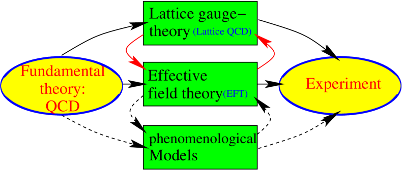
Figure 1: Illustration of different methods to compare properties of QCD to experiment.

In addition to the main lines from EFTs and lattice QCD, there is also shown the path of phenomenological models. The large number of existing quark models fall into this class. The dashed arrows indicate that for those models there is some connection to QCD — often the phrase “QCD inspired models” is used — and observables can be extracted, however, neither is the connection to QCD as rigorous as in the previous two examples nor is it normally possible to systematically improve the calculations. Still, phenomenological models like the non–relativistic quark model, can give important insights and are sometimes even used to estimate the free parameters of the EFTs.

In addition to lattice QCD and EFTs, that allow one to calculate observables from first principles, in special cases also general theorems help to analyze data or to interpret results of calculations. One example of such a theorem applies, if the resonance of interest is located close to an $s$–wave threshold. Then the molecular admixture of this resonance by the corresponding continuum channel can be quantified model-independently. The resulting analysis method is outlined in the next section and applied to various states below. It should be clear that any field theoretical approach has to be consistent with such a general theorem. This holds especially for EFTs as well as lattice QCD. In this case one may use the mentioned theorem to interpret the results of some given calculation. An example of this is given below.

In recent years a large number of narrow states was found in the charm–sector that do not fit into the conventional quark–antiquark picture. An equally large number of non–conventional explanations was proposed for those, including hybrids, glueballs, tetraquarks as well as hadronic molecules (for reviews, see e.g. Refs. [4, 5, 6, 7, 8]), the last ones sometimes appearing as hadro–charmonia — bound systems of $c\bar{c}$ mesons and a light cloud [9]. At present there are no model-independent methods available to disentangle the various scenarios mentioned, besides for the hadronic molecules as outlined in the previous paragraph. Thus, we will focus here on this kind of exotic states.

2 Identifying molecular states

Already 40 years ago Weinberg showed how the molecular content of the deuteron can be quantified [10]. In Ref. [11] it was shown that this result can be generalized even to unstable states as long as their width is narrow and the inelastic thresholds are sufficiently far away. The central result of these studies is that the effective coupling constant of a resonance to a continuum channel in the $s$–wave can be written as

$${\frac{g^{2}_{\rm eff}}{4\pi}} = {4(m_{1}+m_{2})^{2}{\lambda^{2}}\sqrt{2\epsilon/\mu}}+{\cal O}\left(\frac{\sqrt{2\mu\epsilon}}{\beta}\right)$$ (1)

$$\leq 4(m_{1}+m_{2})^{2}\sqrt{2\epsilon/\mu}+{\cal O}\left(\frac{\sqrt{2\mu\epsilon}}{\beta}\right)$$

where $\epsilon=m_{1}+m_{2}-M_{R}$ denotes the binding energy of the resonance $R$, measured relative to the continuum threshold of particle $1$ and $2$, characterized here by their masses $m_{1}$ and $m_{2}$. Further $\mu=m_{1}m_{2}/(m_{1}+m_{2})$ is the reduced mass and $\beta$ denotes the range of forces. Clearly, the formulas given are useful only if the resonance pole is located very near a threshold, for only then the model-dependent corrections that involve the range of forces can safely be neglected. It should also be stressed that for all those states, where the nearby continuum channel is not in an $s$–wave, the scheme can not be applied. The most important parameter in Eq. (1) is $\lambda^{2}$. It gives the probability to find the molecular state in the physical state. Since the effective coupling is an observable, as will also be illustrated in the next paragraph, with Eq. (1) one is in the position to “measure” the amount of the molecular admixture in some physical state. Note, this implies especially that the structure information is hidden in the effective coupling constant, independent of the phenomenology used to introduce the pole(s). Therefore, a successful description of data using some model does not necessarily mean that it is based on correct assumptions. For example, if certain spectra can be described using some isobar model — a model where all dynamics is parameterized by pole terms — it does not mean that all poles deduced are indeed genuine. The poles can as well parameterize singularities of the $S$–matrix generated by hadron–hadron dynamics. A nice illustration of this fact is that one can very well study low energy nuclear physics in an effective theory with an explicit deuteron field [12]. Also in this case, the information on the true nature of the deuteron is hidden in the effective coupling constants in the sense discussed above.

3 The $Y(4660)$ and $Y_{\eta}(4616)$

In order to illustrate how the method described in the previous paragraph works, in this section we will apply it to the $Y(4660)$. This state, discovered using ISR — fixing the quantum numbers to those of the photon, namely $J^{PC}=1^{--}$ — in the $\psi^{\prime}\pi\pi$ final state  [13], is located very near the $f_{0}(980)\psi^{\prime}$ threshold. It is therefore natural to ask, if it is an $f_{0}\psi^{\prime}$ molecule. An important feature of the $Y(4660)$ is that it was neither observed in $e^{+}e^{-}\to\gamma_{ISR}\pi^{+}\pi^{-}J/\psi$ [14], nor in the exclusive $e^{+}e^{-}\to D{\bar{D}},D{\bar{D}}^{*},D^{*}{\bar{D}}^{*},D{\bar{D}}\pi$ cross sections [15], nor in the process $e^{+}e^{-}\to J/\psi D^{(*)}{\bar{D}}^{(*)}$ [16]. In the $f_{0}\psi^{\prime}$ molecular picture, these facts are easy to understand since the molecule would decay mainly through the decays of the unstable $f_{0}(980)$. However, they would severely challenge other models which try to explain the $Y(4660)$ as, for instance, a canonical $5^{3}S_{1}$ $c{\bar{c}}$ charmonium [17] or a baryonium [18].

As outlined above, for a given binding energy and given masses for the constituents, the effective coupling constant of a molecule can be calculated. Thus, it does no longer appear as a parameter in the fit. For the analysis we developed an improved Flatté parameterization that allowed for a consistent inclusion of the spectral function of the $f_{0}$ via a dispersion integral — for details see Ref. [19]. As parameters in the fit to the data now only the mass of the $Y$ and the overall normalization appeared. The fit gave

$$M_{Y}=\left(4665^{+3}_{-5}\right)\ \mbox{MeV}\ .$$ (2)

Clearly, by construction the mass of the $Y(4660)$ is forced to stay below the $f_{0}\psi^{\prime}$ threshold. The result of the fit, shown as the grey band, is compared to the data of Ref. [13] in Fig. 2. The fit is very good. Even the slight asymmetry visible in the data comes out naturally. To confirm that we were not misled by the fitting strategy we performed a second fit, where the effective coupling constant was allowed to float as well. Also this fit called for values of the couplings very near those extracted previously based on the molecular assumption, however, this more relaxed fit allowed for a larger range of masses for the $Y$.

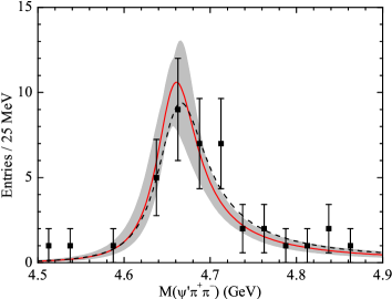
Figure 2: Line shape for the $Y(4660)$ under the assumption of a predominantly molecular nature. The best fit is shown as the solid line, the grey band reflects the 1-$\sigma$ uncertainty of the fit. The dashed line emerges as best fit, if also $g_{\rm eff}$ is allowed to float.

In Ref. [20] it was argued that, if the $Y(4660)$ were an $f_{0}\psi^{\prime}$ molecule, heavy quark spin symmetry predicts a pseudoscalar partner at $M_{Y_{\eta}}=M_{Y}-(M_{\psi^{\prime}}-M_{\eta_{c}^{\prime}})$ being an $f_{0}\eta_{c}^{\prime}$ molecule with very similar properties. Especially the line shape in the $\eta_{c}^{\prime}\pi\pi$ channel should be nearly identical to that shown in Fig. 2. The mass prediction, $M_{Y_{\eta}}=4616^{+5}_{-6}\,$MeV, should hold with very high accuracy, since the spin symmetry breaking terms in case of hadronic molecules with a $c\bar{c}$ constituent are suppressed by an additional factor $1/m_{c}^{2}$ — this emerges since those interactions need to be spin-dependent, connect colour neutral objects, and quark exchange is not possible. The width of the $Y_{\eta}$ into $\eta_{c}^{\prime}\pi\pi$ is predicted to be $\Gamma(\eta_{c}^{\prime}\pi\pi)=(60\pm 30)\,$MeV. An experimental confirmation of this prediction would be very desirable for it would provide further evidence for the picture sketched here.

4 $D_{s0}^{*}(2317)$

So far a method was described that allows one, under certain conditions, to spot molecules under the many states observed. However, the whole scheme was based on non–relativistic quantum mechanics. What we learn from the above is only additional information which states QCD forms, but no direct connection to QCD was employed. As outlined in the introduction, this is possible systematically only using either lattice QCD or effective field theories — more precisely chiral perturbation theory to control the dynamics of mesons formed of light quarks as well as heavy quark effective field theory to construct the interactions amongst heavy fields and, of course, suitable combinations thereof for heavy-light systems.

In this section we will study resonances formed of a light and a heavy meson. However, no perturbative treatment is able to produce poles. Thus we need to leave the ground of rigorous effective field theories and add on top a resummation scheme. The power counting is done of the level of the effective potential so that the convergence of the series has to be checked carefully for the resulting scattering amplitudes and bound state properties, much in the sense outlined by Lepage more than a decade ago [21]. This resummation scheme at the same time has the beneficial side effect that all scattering amplitudes are unitary. Note, this procedure is completely analogous to what is routinely done in case of few–nucleon scattering — for a recent review see Ref. [22].

More precisely, we focus on the scattering of $\pi$, $K$, and $\eta$ off $D$–mesons — see Refs. [23, 24]. Our method is very similar to that of Ref. [25], however, for the first time higher order operators are studied completely and a comparison to lattice data is performed. In addition the poles in the complex plane were identified revealing similar patterns in the heavy-light systems as observed previously for light resonances in Ref. [26].

\psfrag{Vorhersage}{{}}\psfrag{mp}{$m_{\pi}$}\psfrag{c1}{$D\pi\ (I=3/2)$}\psfrag{c2}{$D\bar{K}\ (I=1)$}\psfrag{c3}{$D_{s}K\ (I=1/2)$}\psfrag{c4}{$DK\ (I=0)$}\includegraphics*[width=412.56496pt]{extrapol.eps}

Figure 3: Goldstone boson scattering off $D,D_{s}$-mesons in unitarized chiral perturbation theory. The dashed line shows the result of leading order chiral perturbation theory, while the grey band denotes the results of the full calculation. The lattice data are from Ref. [29].

It is especially important that a complete next–to–leading order calculation was performed which allowed for the first time for a reliable uncertainty estimate, which is, as we will see, especially important in case of the strong width of the $D_{s0}^{*}(2317)$, for here the quark model prediction is significantly lower [31, 32] than that derived within the molecular picture. The scalar charmed–strange meson $D_{s0}^{*}(2317)$ is of particular interest since its observed mass is much lower than the expected value from the non-relativistic quark model [37]. Some ideas were proposed to shift the scalar charmed-strange meson mass down to the mass range of the $D_{s0}^{*}(2317)$. In [38], one loop corrections to the spin-dependent one-gluon exchange potential were considered. Another kind of modification is the mixing of the $c{\bar{s}}$ with the $cq{\bar{s}}{\bar{q}}$ tetraquark [39], or considering the coupling of the $c{\bar{s}}$ to hadronic channels, such as $DK$ [40]. However, such kind of mass shift calculations are model-dependent as pointed out in Refs. [41, 42]. A $KD$ molecular interpretation was proposed by Barnes et al. [43], which agrees with a lot of dynamical calculations [44, 27]. Other exotic explanations were also proposed, such as tetraquark state [45], and $D\pi$ atom [46]. Thus, in order to decide if an experiment can be decisive on the nature of this state, it is necessary that some measure is found to quantify the reliability of the results.

Since the isoscalar $D_{s0}^{*}(2317)$ is located below the $DK$ threshold, the only open strong decay channel is $D_{s}\pi^{0}$, which calls for isospin violation. In QCD there are two sources of isospin violation, namely quark mass differences and electromagnetism. Typically both contribute with similar strength, thus a scheme is necessary for the decays of the $D_{s0}^{*}(2317)$ that allows for a consistent inclusion of both type of effects. This framework is given by chiral perturbation theory. We performed a calculation up to next-to-leading order (NLO). It turned out, although essential for a quantitative understanding of the $D^{0}$, $D^{+}$ mass difference, electromagnetic effects played a minor role in the strong decay of the $D_{s0}^{*}(2317)$ — thus the decay was dominated by $\pi^{0}-\eta$ mixing, first shown in Ref. [27] to give a width of 8 keV, as well as the $D$–meson mass differences in the loops, studied previously in Refs. [28, 25], which, when added in, give a width of 180 keV. On the contrary in case of a pure quark state the meson loop contribution is absent and thus a width of about 8 keV is predicted [32]. Similar values are expected for all other non–molecular scenarios. Thus, there is a direct experimental test available for the conjecture that the $D_{s0}^{*}(2317)$ is a hadronic molecule.

Unfortunately, the uncertainty of 110 keV turns out to be quite large. However, this uncertainty originates solely form the poorly determined isospin conserving interactions — to the order we are working all isospin breaking terms could be fixed from other sources. However, there are other tools to reduce the uncertainty on the isospin conserving part, namely by comparing to lattice QCD. For this comparison scattering lengths (i.e the scattering amplitudes at threshold) are ideal: on the one hand they can be calculated on the lattice by systematic studies of the volume dependence of correlators [30] and on the other hand they can be straightforwardly calculated on the basis of (unitarized) chiral perturbation theory. The predictions of our calculation are shown in Fig. 3 as a function of the pion mass. The dashed line shows the result of leading order chiral perturbation theory, while the grey band denotes the results of the full calculation. The lattice data are from Ref. [29]. Note that in the lattice calculations only the light quark mass was varied while the strange quark mass was kept fixed close to its physical value — this is why for vanishing $m_{\pi}$ only the scattering length for $\pi D$ scattering vanishes, as demanded by the Goldstone theorem. As can be seen, in all channels our calculation agrees very well with the lattice results. The expansion appears to converge very well for $\pi D$ scattering, while in case of $D\bar{K}$ and $D_{s}K$ scattering in the $I=1$ and $I=1/2$ channels, respectively, up to 50% corrections emerged from higher orders. Although quite sizable, even this change is within the expectations from the power counting as a result of the relatively large kaon mass. However, in case of $KD$ scattering in the isoscalar channel the change is truely dramatic — the scattering length even changes its sign. This change in sign, clearly a non–perturbative effect, is a consequence of the appearance of the $D_{s0}^{*}(2317)$ as a $KD$ bound state. In this context it is important to remember the theorem stated above that for bound states the effective coupling constant can be calculated directly from masses, the binding energy and $\lambda^{2}$, the probability to find the molecular state in the physical state — c.f. Eq. (1). This property translates directly into a prediction for the scattering length, if the binding energy of the bound state is small. In this case the scattering length may be written as

$$a\simeq\frac{-2\lambda^{2}/(1+\lambda^{2})}{\sqrt{2m_{K}\epsilon}}\ .$$ (3)

And indeed, the value we predict for the $KD$ scattering length exactly agrees with the prediction from the general theorem in case of a purely molecular nature of the $D_{s0}^{*}(2317)$ ($\lambda^{2}=0$). This opens the opportunity to extract the nature of the $D_{s0}^{*}(2317)$ directly from a lattice study: if this study were to find a scattering length in this channel of about $-1$ fm, it would prove the nature of the $D_{s0}^{*}(2317)$ as a $KD$ molecule. A larger absolute value of the scattering length is not allowed, while any smaller value would immediately quantify a non–molecular admixture — see Eq. (3). This equation also embodies the concept of universality for large scattering length, for a lucid review see [47].

Above we argued that lattice data can be used to determine the LECs of chiral perturbation theory. How this could work in the future can also be read off Fig. 3. At present both the theoretical predictions as well as the lattice data show a significant scatter. In addition, so far the lattice studies were performed only for one lattice spacing. Further investigations are necessary to quantify the systematics of the analysis and also adding more points for pion masses below 300 MeV. However, we hope that soon the lattice data/analysis will improve and then the parameters of our theoretical study can be constrained by a fit to those data (this calls for a complete theoretical calculation to NNLO, however, which still needs to be done). Once this is done, one can expect that the theoretical uncertainty of the prediction for the width of the $D_{s}(2317)$ is reduced significantly as well.

5 Discussion

If mesonic bound states exist at all, shouldn’t one expect a large number of those in the spectrum? First of all one should stress that hadron dynamics normally produces sufficient attraction only in very few channels. This can also be seen, e.g., in Fig. 3: in all channels displayed, besides the $KD$ $I=0$ channel, where the $D_{s0}^{*}(2317)$ can be found, the interaction is repulsive. In addition, there may already exist various molecules in both, the light sector (here, e.g., the $f_{0}(980)$ is a prominent candidate for a $\bar{K}K$ molecule [33], not only because of its mass close to the $\bar{K}K$ threshold but also because of its properties [11, 34]) as well as in the charm sector. Here the most prominent candidate not discussed in this contribution is the $X(3872)$ as a prime candidate for a $D^{*}\bar{D}+h.c.$ molecule (see Ref. [35] and references therein) or virtual state, possibly with some $c\bar{c}$ admixture (see Refs. [36] and references therein). In this contribution we outlined under what circumstances it is possible to get model-independent statements about the molecular nature of states — this is especially possible for states located very close to an $s$–wave threshold. However, models predict many more states. E.g. a brother of the $Y(4660)$ discussed above as a candidate for a $f_{0}\psi^{\prime}$ bound state, could be the $Y(4260)$ in Ref. [48] claimed to the a resonance of $f_{0}(980)$ and $J/\psi$. In Refs. [49, 50] similar conclusions are drawn based on QCD sum rules.

On the long run we will be able to address these issues, namely through the mentioned interplay of general theorems, lattice QCD as well as effective field theories. As was shown in Ref. [26], there are cases where it is possible to move a resonance, by changing a QCD parameter — here the quark mass — from a position deep in the complex plane to a kinematic situation where the bound state analysis sketched above can be applied. The precondition for this is clearly to have a formalism which allows for a controlled quark mass dependence. The parametric dependence of resonances on QCD parameters can also be checked in a study of the corresponding form factors [52]. This investigation provides an additional check of the systematics of the approaches. In this sense we can hope to get a deeper understanding of QCD in the non–perturbative regime, once improved experimental data are available to check and refine the theoretical approaches.

References

- [1] U.-G. Meißner and G. Schierholz, arXiv:hep-ph/0611072.
- [2] D. Kadoh et al. [PACS-CS Collaboration], arXiv:0810.0351 [hep-lat].
- [3] S. R. Sharpe, arXiv:hep-lat/0607016.
- [4] E. S. Swanson, Phys. Rept. 429 (2006) 243 [arXiv:hep-ph/0601110].
- [5] E. Klempt and A. Zaitsev, Phys. Rept. 454 (2007) 1 [arXiv:0708.4016 [hep-ph]].
- [6] M. B. Voloshin, Prog. Part. Nucl. Phys. 61 (2008) 455 [arXiv:0711.4556 [hep-ph]].
- [7] S. Godfrey and S. L. Olsen, Ann. Rev. Nucl. Part. Sci. 58 (2008) 51 [arXiv:0801.3867 [hep-ph]].
- [8] E. Braaten, arXiv:0808.2948 [hep-ph].
- [9] S. Dubynskiy and M. B. Voloshin, Phys. Lett. B 666 (2008) 344 [arXiv:0803.2224 [hep-ph]].
- [10] S. Weinberg, Phys. Rev. 130 (1963) 776; 131 (1963) 440; 137 (1965) B672.
- [11] V. Baru et al., Phys. Lett. B 586 (2004) 53.
- [12] D. B. Kaplan, Nucl. Phys. B 494 (1997) 471 [arXiv:nucl-th/9610052].
- [13] X. L. Wang et al. [Belle Collaboration], Phys. Rev. Lett. 99 (2007) 142002 [arXiv:0707.3699 [hep-ex]].
- [14] C. Z. Yuan et al. [Belle Collaboration], Phys. Rev. Lett. 99 (2007) 182004 [arXiv:0707.2541 [hep-ex]].
- [15] K. Abe et al. [Belle Collaboration], Phys. Rev. Lett. 98 (2007) 092001 [arXiv:hep-ex/0608018]; G. Pakhlova et al. [Belle Collaboration], Phys. Rev. Lett. 100 (2008) 062001 [arXiv:0708.3313 [hep-ex]]; G. Pakhlova et al. [Belle Collaboration], Phys. Rev. D 77 (2008) 011103 [arXiv:0708.0082 [hep-ex]]; B. Aubert et al. [BABAR Collaboration], arXiv:0710.1371 [hep-ex].
- [16] P. Pakhlov et al. [Belle Collaboration], Phys. Rev. Lett. 100 (2008) 202001 [arXiv:0708.3812 [hep-ex]].
- [17] G. J. Ding, J. J. Zhu and M. L. Yan, Phys. Rev. D 77, 014033 (2008) [arXiv:0708.3712 [hep-ph]].
- [18] C. F. Qiao, J. Phys. G 35 (2008) 075008 [arXiv:0709.4066 [hep-ph]].
- [19] F. K. Guo, C. Hanhart and U.-G. Meißner, Phys. Lett. B 665 (2008) 26 [arXiv:0803.1392 [hep-ph]].
- [20] F. K. Guo, C. Hanhart and U.-G. Meißner, Phys. Rev. Lett. 102 (2009) 242004 [arXiv:0904.3338 [hep-ph]].
- [21] G. P. Lepage, arXiv:nucl-th/9706029.
- [22] E. Epelbaum, H. W. Hammer and U.-G. Meißner, arXiv:0811.1338 [nucl-th], Rev. Mod. Phys., in print.
- [23] F. K. Guo, C. Hanhart and U.-G. Meißner, Eur. Phys. J. A 40 (2009) 171 [arXiv:0901.1597 [hep-ph]].
- [24] F. K. Guo, C. Hanhart, S. Krewald and U.-G. Meißner, Phys. Lett. B 666 (2008) 251 [arXiv:0806.3374 [hep-ph]].
- [25] M. F. M. Lutz and M. Soyeur, Nucl. Phys. A 813 (2008) 14 [arXiv:0710.1545 [hep-ph]].
- [26] C. Hanhart, J. R. Pelaez and G. Rios, Phys. Rev. Lett. 100 (2008) 152001 [arXiv:0801.2871 [hep-ph]].
- [27] F. K. Guo, P. N. Shen, H. C. Chiang and R. G. Ping, Phys. Lett. B 641 (2006) 278 [arXiv:hep-ph/0603072].
- [28] A. Faessler, T. Gutsche, V. E. Lyubovitskij and Y. L. Ma, Phys. Rev. D 76 (2007) 014005 [arXiv:0705.0254 [hep-ph]].
- [29] L. Liu, H. W. Lin and K. Orginos, PoS LATTICE 2008 (2008) 112 [arXiv:0810.5412 [hep-lat]].
- [30] M. Luscher, Commun. Math. Phys. 105 (1986) 153.
- [31] S. Godfrey, Phys. Lett. B 568 (2003) 254 [arXiv:hep-ph/0305122].
- [32] F. de Fazio, talk presented at this conference.
- [33] J. D. Weinstein and N. Isgur, Phys. Rev. D 41 (1990) 2236.
- [34] Yu. S. Kalashnikova, A. E. Kudryavtsev, A. V. Nefediev, C. Hanhart and J. Haidenbauer, Eur. Phys. J. A 24 (2005) 437 [arXiv:hep-ph/0412340]; C. Hanhart, Yu. S. Kalashnikova, A. E. Kudryavtsev and A. V. Nefediev, Phys. Rev. D 75 (2007) 074015 [arXiv:hep-ph/0701214].
- [35] E. Braaten and M. Lu, Phys. Rev. D 76 (2007) 094028 [arXiv:0709.2697 [hep-ph]].
- [36] C. Hanhart, Yu. S. Kalashnikova, A. E. Kudryavtsev and A. V. Nefediev, Phys. Rev. D 76 (2007) 034007 [arXiv:0704.0605 [hep-ph]]; Yu. S. Kalashnikova and A. V. Nefediev, arXiv:0907.4901 [hep-ph].
- [37] S. Godfrey and N. Isgur, Phys. Rev. D 32 (1985) 189.
- [38] O. Lakhina and E. S. Swanson, Phys. Lett. B 650 (2007) 159 [arXiv:hep-ph/0608011].
- [39] T. E. Browder, S. Pakvasa and A. A. Petrov, Phys. Lett. B 578 (2004) 365 [arXiv:hep-ph/0307054]; J. Vijande, F. Fernandez and A. Valcarce, Phys. Rev. D 73 (2006) 034002 [Erratum-ibid. D 74 (2006) 059903] [arXiv:hep-ph/0601143].
- [40] E. van Beveren and G. Rupp, Phys. Rev. Lett. 91 (2003) 012003 [arXiv:hep-ph/0305035]; Phys. Rev. Lett. 97 (2006) 202001 [arXiv:hep-ph/0606110]; D. S. Hwang and D. W. Kim, Phys. Lett. B 601 (2004) 137 [arXiv:hep-ph/0408154]; Yu. A. Simonov and J. A. Tjon, Phys. Rev. D 70 (2004) 114013 [arXiv:hep-ph/0409361].
- [41] S. Capstick et al., Eur. Phys. J. A 35 (2008) 253 [arXiv:0711.1982 [hep-ph]].
- [42] F. K. Guo, S. Krewald and U.-G. Meißner, Phys. Lett. B 665 (2008) 157 [arXiv:0712.2953 [hep-ph]].
- [43] T. Barnes, F. E. Close and H. J. Lipkin, Phys. Rev. D 68 (2003) 054006 [arXiv:hep-ph/0305025].
- [44] E. E. Kolomeitsev and M. F. M. Lutz, Phys. Lett. B 582 (2004) 39 [arXiv:hep-ph/0307133]; J. Hofmann and M. F. M. Lutz, Nucl. Phys. A 733 (2004) 142 [arXiv:hep-ph/0308263]; Y. J. Zhang, H. C. Chiang, P. N. Shen and B. S. Zou, Phys. Rev. D 74 (2006) 014013 [arXiv:hep-ph/0604271]; D. Gamermann, E. Oset, D. Strottman and M. J. Vicente Vacas, Phys. Rev. D 76 (2007) 074016 [arXiv:hep-ph/0612179].
- [45] H. Y. Cheng and W. S. Hou, Phys. Lett. B 566 (2003) 193 [arXiv:hep-ph/0305038]; K. Terasaki, Phys. Rev. D 68 (2003) 011501 [arXiv:hep-ph/0305213]; Y. Q. Chen and X. Q. Li, Phys. Rev. Lett. 93 (2004) 232001 [arXiv:hep-ph/0407062]; L. Maiani, F. Piccinini, A. D. Polosa and V. Riquer, Phys. Rev. D 71 (2005) 014028 [arXiv:hep-ph/0412098]; U. Dmitrasinovic, Phys. Rev. Lett. 94 (2005) 162002; H. Kim and Y. Oh, Phys. Rev. D 72 (2005) 074012 [arXiv:hep-ph/0508251]; M. Nielsen, R. D. Matheus, F. S. Navarra, M. E. Bracco and A. Lozea, Nucl. Phys. Proc. Suppl. 161 (2006) 193 [arXiv:hep-ph/0509131]; Z. G. Wang and S. L. Wan, Nucl. Phys. A 778 (2006) 22 [arXiv:hep-ph/0602080].
- [46] A. P. Szczepaniak, Phys. Lett. B 567 (2003) 23 [arXiv:hep-ph/0305060].
- [47] E. Braaten and H. W. Hammer, Phys. Rept. 428 (2006) 259 [arXiv:cond-mat/0410417].
- [48] A. Martinez Torres, K. P. Khemchandani, D. Gamermann and E. Oset, arXiv:0906.5333 [nucl-th].
- [49] Z. G. Wang and X. H. Zhang, arXiv:0905.3784 [hep-ph].
- [50] Z. G. Wang and X. H. Zhang, arXiv:0908.2003 [hep-ph].
- [51] P. C. Bruns and U.-G. Meißner, Eur. Phys. J. C 40 (2005) 97 [arXiv:hep-ph/0411223]; P. C. Bruns and U.-G. Meißner, Eur. Phys. J. C 58 (2008) 407 [arXiv:0808.3174 [hep-ph]].
- [52] F. K. Guo, C. Hanhart, F. J. Llanes-Estrada and U.-G. Meißner, Phys. Lett. B 678 (2009) 90 [arXiv:0812.3270 [hep-ph]].