Geometrical foundations of plasticity yield criteria: A unified theory

Abstract

A new model for elucidating the mathematical foundation of plasticity yield criteria is proposed. The proposed ansatz uses differential geometry and group theory concepts in addition to elementary hypotheses based on well-established experimental evidence. Its theoretical development involves the analysis of tensor functions and provides a series expansion which allows the functional stress-dependence of plasticity yield criteria to be predicted. The theoretical framework for the model includes a series of spatial coefficients that provide a more flexible theory for in-depth examination of symmetry and anisotropy in compact solid materials. It describes the classical yield criteria (like those of Tresca, Von Mises, Hosford, Hill, etc) and accurately describes the anomalous behaviour of metals such as aluminium, which was elucidated by Hill (1979). Further, absolutely new instances of stress-dependence are predicted; this makes it highly useful for fitting experimental data with a view to studying the phenomena behind plasticity.

Keywords: geometrical model, analytic functions, manifold, anisotropic material, elastic-plastic material

1 Introduction

An accurate description of the structure, formation and behaviour of a solid elastic-plastic material requires the knowledge, among other facts, of the limiting stress it can withstand before it becomes plastic [32, 33, 15, 18, 2, 22]. In fact, plasticity concepts are widely used in a number of scientific and engineering field applications (in materials science, physics of solids, mechanical engineering, aeronautical engineering, geophysics, biomechanics and chemistry, among others) [4, 8, 1].

Plasticity involves a series of irreversible, history-dependent processes by effect of which a material develops fluency at a micro-, meso- or macroscopic scale in its transition from an elastic behaviour to a plastic behaviour [26]. Plastic processes involve plastic dissipation (i.e., the irreversible release of stress or energy with energy transfer in the material). In fact, plasticity involves a variety of processes at different spatial scales having an also different associated grain size. In addition to its physical reality to plastic processes, grain size defines characteristic spatial scales for macroscopic plasticity in materials [19].

Unlike liquids and gases, solids are highly ordered systems, contain a vast amount of internal information and exhibit a high correlation among its constituent elements. As a result, plastic microscopic processes in solids (movement of dislocations, defect, etc) are usually relatively complex [19]. However, such processes exhibit some macroscopic symmetry by virtue of the solids structure and the physical laws they obey [4, 26, 5, 6]. This facilitates the macroscopic examination of solids by using a combination of differential geometry and group theory [3, 30]. Thus, a plastic process can be interpreted as a series of local transformations that possess some symmetry and provide local information useful with a view to establishing a global statistics for a solid material.

The aim of this paper is to develop a unified approach of plasticity yield criteria that uses elementary hypotheses based on well-established experimental evidence. This study is based on the analysis of the transformation properties of the Cauchy stress tensor under orthogonal mappings, where arguments from the theory of Lie groups are applied. Also, it discusses the physical arguments for application of each criterion in relation to specific properties of the material concerned. This can be useful with a view to developing new criteria to address some special mechanical properties of materials (like anisotropy, hardening-softening, etc).

This paper is organized as follows. Section 2 describes some topics about plasticity in the framework of the internal variables theory. Section 3 presents a short description of classical plasticity criteria. In section 4 we show the postulates and approximations of the unified theory. From section 5 onwards we develop this unified theory. Finally, a set of conclusions is shown.

2 Plasticity function and plastic potential. Flow rule

Within the framework of the Internal Variables Theory (or hidden variables), an inelastic solid is one in which the strain at any point of the solid is completely determined by the current stress and temperature there plus a set of internal variables [26, 28]. The internal variables (scalars or tensors) have physical or mathematical meaning and allow to complete the internal description at any point of the solid (for example: the past history of the stress and temperature at the point, large-deformation plasticity, hardening and softening, structural and induced anisotropy, etc) [26, 29]. Thus $\varepsilon$ is a function of the material state $(\sigma,T,\xi)$ at any point

$$\varepsilon=\varepsilon(\sigma,T,\xi)$$ (1)

where $\varepsilon$ denotes strain variables, $\sigma$ stress variables, $T$ the temperature, and $\xi$ some internal variables. Additionally, the rate of evolution of the internal variables $\dot{\xi}$ is determined by the state

$$\dot{\xi}=\dot{\xi}(\sigma,T,\xi)$$ (2)

known like equations of evolution or rate equation for internal variables.

For inelastic solids it is generally assumed that strain variables can be decomposed additively into elastic strain $\varepsilon^{e}$ and inelastic strain $\varepsilon^{i}$ [8]

$$\varepsilon=\varepsilon^{e}+\varepsilon^{i}$$ (3)

where the inelastic strain occurring in rate-independent plasticity is usually denoted by $\varepsilon^{P}$rather than by $\varepsilon^{i}$, and is called the plastic strain.

In the context of internal variables theory and rate-independent plasticity, a plasticity yield criterion consists of a series of mathematical conditions mutually relating stress, temperature and internal variables, which define the material states $(\sigma,T,\xi)$, where the point of the solid concerned becomes critically plastic. A critical state in this context is a state where the elastic-plastic material starts to yield plasticity. Therefore, these conditions constitute a boundary (plastic limit) between the elastic and plastic state in the solid material (at points). Mathematically, plasticity yield criteria are formulated in the following general form:

$$f(\sigma,T,\xi)=0$$ (4)

where $f$ denotes the plasticity function at a given plastic state $(\sigma,T,\xi)$. Therefore, the plasticity yield criterion of a solid (at points) defines the stress multiaxial states where it will yield critical plasticity; the set of such states describes the criterion surface of the solid (4).

Plasticity can be defined in basic terms by using some approximations that usually hold in practice. Thus, the influence of the temperature $T$ on solids at a constant, ambient level is usually negligible provided they are scarcely sensitive to changes in this variable and far from their melting point (temperature-independent plasticity). The influence of strain is usually negligible if we consider all viscoplastic processes to be “infinitely” slow compared to the material relaxation time (rate-independent plasticity) [26]. Time-independent plasticity needs usually to be considered if the target is not the time-evolution of the solid. In the plastic limit, an index $P$ is used to denote parameters and quantity values in such a limit. The basic plastic unit in a solid is the macroscopic spatial point, which can be equated to the physical concept of grain but need not coincide with it. Also, because a solid usually exhibits high correlation among its elements, characterizing each point in it requires defining its correlation with its neighbourhood. As in the theory of elasticity, this entails describing the stress state at each point in terms of a second-order symmetric tensor (2-tensor) $\sigma\equiv\sigma_{ij}$, called the Cauchy tensor, the symmetry of which arises from the stress equilibrium relation at the point in question [24]. Therefore, in these conditions, the plasticity yield criterion (4) at each point in a solid can be defined as follows:

$$f(\sigma_{ij};\xi)=0$$ (5)

which represents the criterion surface in the stress space.

The plastic potential, $\Phi$, is a measure of smoothness (differentiability) and convexity of $f$. Thus, if the plasticity function $f$ is smooth (differentiable) and convex in stress space, then it will coincide with a specific plastic potential ($f=\Phi$). The plasticity function $f=\Phi$ is convex if for a given stress and strain rate condition $\sigma_{ij}$ and $\dot{\varepsilon}_{ij}^{P}$, any stress $\sigma_{ij}^{*}$ inside or on the criterion surface obeys the following relationship [26]:

$$(\sigma_{ij}-\sigma_{ij}^{*})\dot{\varepsilon}_{ij}^{P}\geq 0$$ (6)

where $\dot{\varepsilon}_{ij}^{P}$ denotes the plastic strain rate. Specifically, if $f=\Phi$ is twice differentiable, then $\Phi$ will be convex if, and only if, its Hessian matrix, defined as

$$H_{ij}=\frac{\partial^{2}\Phi}{\partial\sigma_{i}\partial\sigma_{j}}$$ (7)

is positive semi-definite (i.e. if the eigenvalues of $H_{ij}$ are only positive or zero). When the eigenvalues are only positive non-zero (positive definite matrix), $f=\Phi$ is strictly convex. We have used here —as we have throughout— the Einstein summation convention for repeated indices.

If $f$ is smooth (differentiable) and convex, then $\dot{\varepsilon}_{ij}^{P}$ will be unique in any plastic stress state $\sigma_{ij}$. Under these conditions, the function $f=\Phi$ can be assigned a flow rule that gives the plastic strain rate. Within the framework of the plastic potential theory of Von Mises (1928), each plastic potential $\Phi$ has a flow rule that is associated with the plastic potential. This flow rule is given by

$$\dot{\varepsilon}_{ij}^{P}=\dot{\lambda}\frac{\partial\Phi}{\partial\sigma_{ij}}$$ (8)

where $\sigma_{ij}$ is the Cauchy tensor, $\dot{\varepsilon}_{ij}^{P}$ the plastic strain rate tensor or plastic flow tensor and $\dot{\lambda}$ a positive plastic multiplying factor. Based on eq. (8), if $f=\Phi$, then the plastic strain rate $\dot{\varepsilon}_{ij}^{P}$ at the very start of plasticity will be normal to the criterion surface $f=\Phi$; this constitutes the so-called plastic flow normality rule. Hecker [13] conducted a systematic study of a large amount of experimental data in metals and found that the normality rule was never broken. However, there is evidence that flow normality rule does not hold in soils, granular materials, etc (materials with non-associated flow rules, where $\partial f/\partial\sigma_{ij}$ is not proportional to $\partial\Phi/\partial\sigma_{ij}$) [8, 26].

Defining rate-independent plasticity requires introducing the concept of plastic dissipation, which is expressed as

$$d=\sigma_{ij}\dot{\varepsilon}_{ij}^{P}$$ (9)

The parameter $d$ is a measure of the power per volume that is lost (dissipated), usually as heat, through deformation. The plastic dissipation as defined in eq. (9) for the flow rule associated to $f$ will be maximal if, and only if, the function $f=\Phi$ is convex (9); this is the so-called principle of maximum plastic dissipation [31, 16].

Establishing the total dissipation over a given time interval entails defining in terms of time-dependent plasticity the amount of irreversible work per unit volume due to stress as follows:

$$\chi(t)=W^{P}(t)=\int_{0}^{t}\sigma_{ij}(t)\dot{\varepsilon}_{ij}^{P}(t)dt$$ (10)

$\chi(t)$ is also known as the work-hardening parameter (an internal variable), which is a scalar quantity and dependent on the plastic time-evolution of the particular solid.

For the study of the hardening and softening of the solids materials is necessary the evolution of plasticity function with the internal variables, $\xi=\xi_{\alpha}$, given by [26]

$$\left.\dot{f}\right|_{\sigma=const.,\;T=const.}=\sum_{\alpha}\frac{\partial f}{\partial\xi_{\alpha}}\dot{\xi}_{\alpha}=\lambda\sum_{\alpha}\frac{\partial f}{\partial\xi_{\alpha}}h_{\alpha}\equiv-\lambda H$$ (11)

where $H>0$ for hardening materials, $H<0$ for softening materials, and $H=0$ for perfectly plastic materials (in the latter case $f$ is independent of the $\xi_{\alpha}$). Here $\lambda$ is a positive continuous function of state variables.

Based on the foregoing, for the theory to be properly addressed, the plasticity function $f$ should be convex in the stress-related variables ($f=\Phi$). The dependency of $f$ on $\xi$ describes the anisotropy (structural and induced) of materials, while the dependency of $\dot{f}$ on $\xi$ describes the hardening-softening of materials.

3 Plasticity yield criteria

The following section describes the most relevant plasticity yield criteria, with emphasis on their particularities (see [32, 33, 15, 18, 2, 22]).

The Tresca criterion [32] which is among the earliest plasticity yield criteria, can be expressed as a unique function of the algebraic invariants $(J_{1},J_{2},J_{3})$ of the stress deviation tensor $J$. Based on it, a solid will become plastic when it reaches a multiaxial state where the multiaxial tangent stress equals the critical uniaxial tangent stress, $\sigma_{P}$. This criterion can be expressed as a completely differentiable relation

$$f(\sigma_{ij};\sigma_{P}) =\left[(\sigma_{xx}-\sigma_{yy})^{2}+4\sigma_{xy}^{2}-4\sigma_{P}^{2}\right][\left(\sigma_{yy}-\sigma_{zz})^{2}+4\sigma_{yz}^{2}-4\sigma_{P}^{2}\right]$$ (12)

$$\times[\left(\sigma_{zz}-\sigma_{xx})^{2}+4\sigma_{xz}^{2}-4\sigma_{P}^{2}\right]$$

based on which plasticity can only be reached on independent planes, as revealed by factoring the total (volume) multiaxial state into its partial (surface) multiaxial state. In other words, plasticity develops on planes. This criterion exhibits good agreement with experimental results for certain ductile metals. At microscopic level the movement of dislocations along slip planes is responsible for permanent deformation [4]. Note that $\sigma_{P}$ depends on the internal variables, $\xi$, i.e. $\sigma_{P}=\sigma_{P}(\xi)$.

The Huber–Von Mises criterion [33, 21] is among the most widely rule used in this context. It is also known as the $J_{2}$-criterion since it is formulated as a unique function of the algebraic invariant $J_{2}$ of the stress deviation tensor. Based on existing experimental evidence, this criterion is applicable to ductile materials. Hencky [14] provided an energy-based interpretation by which the critical plasticity state is reached when the distortion energy per volume (i.e., the deformation energy per volume in the absence of volume changes) in the multiaxial tangent stress state equals the distortion energy per volume in the critical uniaxial normal stress state. This criterion is isotropic and can be formulated as follows:

$$f(\sigma{}_{ij};\sigma_{P})=(\sigma_{xx}-\sigma_{yy})^{2}+(\sigma_{yy}-\sigma_{zz})^{2}+(\sigma_{zz}-\sigma_{xx})^{2}+6(\sigma_{xy}^{2}+\sigma_{yz}^{2}+\sigma_{xz}^{2})-2\sigma_{P}^{2}$$ (13)

Stress-wise, the Von Mises criterion indicates that critical plasticity is reached when the modulus of the multiaxial tangent stress equals that of the critical uniaxial normal stress, $\sigma_{P}$. Note that $\sigma_{P}$ depend on the internal variables, $\xi$, i.e. $\sigma_{P}=\sigma_{P}(\xi)$. Unlike the Tresca criterion, the Von Mises criterion does not factor the plasticity function into multiaxial plane stress components; rather, it assumes a mutual dependence among the multiaxial stresses, which leads to a volume plasticity expression. In ductile materials, which meet the Von Mises criterion quite well, plasticity results in distortion by effect of flow processes occurring with virtually no volume change.

The Hill’s anisotropic criterion or Hill’s first criterion [15, 17] provides a general description of materials with anisotropy (whether structural or induced) and orthotropic symmetry (i.e., materials where each point possess three mutually normal planes). Because each plane in an orthotropic material can be defined in terms of only two parameters, Hill’s criterion can be formulated in terms of six independent parameters. This constitutes a generalization of the Von Mises criterion to anisotropic materials of the form

$$A(\sigma_{yy}-\sigma_{zz})^{2}+B(\sigma_{zz}-\sigma_{xx})^{2}+C(\sigma_{xx}-\sigma_{yy})^{2}+2D\sigma_{yz}^{2}+2E\sigma_{xz}^{2}+2F\sigma_{xy}^{2}=1$$ (14)

where $A=A(\xi),B=B(\xi),C=C(\xi),D=D(\xi),E=E(\xi),F=F(\xi)$, depending on the internal variables, are constants defining the degree of anisotropy in each direction and can be expressed in terms of the Lankford coefficient. In addition, the directions $x,y,z$ should be the principal anisotropy directions for the material —otherwise, the Cauchy tensor should be transformed as required in order to have it coincide with the principal directions. In fact, eq. (14) is a particular case [26] of

$$\sigma_{ij}B_{ijkl}\sigma_{kl}=\sigma_{P}^{2}$$ (15)

which is the more general quadratic form for the components of the stress tensor as defined in terms of the 4-tensor $B_{ijkl}$. This tensor fulfils the symmetry conditions for 4-tensors in the theory of elasticity, which are given by

$$\begin{array}[]{l}{B_{ijkl}=B_{klij}}\\ {B_{ijkl}=B_{jikl}}\end{array}$$ (16)

where the first relation defines the symmetry by joint exchange of index pairs $ij\leftrightarrow kl$ and the second the symmetry by exchange between index pairs of the type $i\leftrightarrow j$ and/or $k\leftrightarrow l$. This criterion considers no effects of the mean stress (hydrostatic pressure) on plasticity; therefore, one must introduce the additional condition $B_{ijkk}=0$, which allows the quadratic form of such effects to be neglected.

The Hosford criterion [20] and Logan–Hosford criterion [25] are two generalizations of the Von Mises criterion that ensure convexity by introducing a parameter $m\geq 1$. The Hosford criterion, which is applicable to isotropic materials, is defined as

$$f(\sigma_{ij};\sigma_{P})=\frac{1}{2}\left|\sigma_{1}-\sigma_{2}\right|^{m}+\frac{1}{2}\left|\sigma_{2}-\sigma_{3}\right|^{m}+\frac{1}{2}\left|\sigma_{1}-\sigma_{3}\right|^{m}-\sigma_{P}^{m}$$ (17)

where $\sigma_{1},\sigma_{2},\sigma_{3}$ are the principal stresses of the Cauchy tensor. Note that $\sigma_{P}$ depends on the internal variables,$\sigma_{P}=\sigma_{P}(\xi)$. The Logan–Hosford criterion is a generalization of Hill’s anisotropic criterion (14) that is used to describe anisotropic materials and expressed as

$$A{{}^{\prime}}\left|\sigma_{1}-\sigma_{2}\right|^{m}+B{{}^{\prime}}\left|\sigma_{2}-\sigma_{3}\right|^{m}+C{{}^{\prime}}\left|\sigma_{1}-\sigma_{3}\right|^{m}=1$$ (18)

where the constants $A{{}^{\prime}}=A{{}^{\prime}}(\xi),B{{}^{\prime}}=B{{}^{\prime}}(\xi),C{{}^{\prime}}=C{{}^{\prime}}(\xi)$, depending on the internal variables, constitute measures of anisotropy in each direction and can be expressed as a function of the Lankford coefficient.

Hill’s generalized anisotropic criterion or Hill’s second criterion [18] provides an accurate description of the anomalous behaviour of some metals such as aluminium [37]. The criterion is expressed in terms of principal stresses of the Cauchy tensor:

$$a\left|\sigma_{2}-\sigma_{3}\right|^{m}+b\left|\sigma_{3}-\sigma_{1}\right|^{m}+c\left|\sigma_{1}-\sigma_{2}\right|^{m}+d\left|2\sigma_{1}-\sigma_{2}-\sigma_{3}\right|^{m}+$$

$$e\left|2\sigma_{2}-\sigma_{1}-\sigma_{3}\right|^{m}+f\left|2\sigma_{3}-\sigma_{1}-\sigma_{2}\right|^{m}=\sigma_{P}^{m}$$ (19)

where $m\in\Re$ is a parameter that must fulfil the condition $m\geq 1$ for the criterion surface to be convex. Also the constants $a=a(\xi),b=b(\xi),c=c(\xi),d=d(\xi),e=e(\xi),f=f(\xi),\;\sigma_{P}=\sigma_{P}(\xi)$ depending on the internal variables, $\xi$, and which can be expressed as a function of the Lankford coefficient, measure anisotropy in each principal direction. For example, if the principal directions 1–2 in a material define a symmetry plane with mutual isotropy and are anisotropic with respect to direction 3, then $a=b$ and $d=e$ (planar isotropy). On the other hand, if all three directions are isotropic, then $a=b=c$ and $d=e=f$ (complete isotropy).

In the plastic potential theory of Von Mises [34], each plastic potential $\Phi$ is assigned a flow rule. The plastic potential for the particular case of the Von Mises criterion is $J_{2}$ and its associated flow rule defined by the Levy–Mises equations. Koiter [23] developed a generalization of the previous theory where the plasticity function is defined by a series of plastic potentials $\Phi_{i}$ each having an associated flow rule of the type described by eq. (8) above. If the plasticity function $f$ is expressed as a linear combination with positive coefficients of the potential functions $\Phi_{i}$ (convex), then $f$ will be convex.

The plastic anisotropy description of Barlat et al. [2] originated from an isotropic plasticity function. Structural anisotropy in the material was introduced via a series of linear transformations represented by a 4-tensor acting on the Cauchy tensor, the latter itself acting on the anisotropic material. By effect of the transformations, the stress tensor absorbs structural anisotropy of the material.

The Karafillis–Boyce criterion [22] uses a convex combination of two plastic potentials as plasticity function. The potentials are based on Hosford’s isotropic criterion (17) and their degree of mixing is adjusted via parameter $c\in[0,1]$. Thus, the isotropic criterion is formulated as

$$(1-c)\left[\left|s_{1}-s_{2}\right|^{m}+\left|s_{2}-s_{3}\right|^{m}+\left|s_{3}-s_{1}\right|^{m}\right]+c\frac{3^{m}}{2^{m-1}+1}\left[\left|s_{1}\right|^{m}+\left|s_{2}\right|^{m}+\left|s_{3}\right|^{m}\right]=2\sigma_{P}^{m}$$ (20)

where $m$ is positive and non-zero, and $s_{1},s_{2},s_{3}$ are the principal values (eigenvalues) of the stress deviation tensor. Note that $\sigma_{P},\;c$ depend on the internal variables, $\sigma_{P}=\sigma_{P}(\xi),\;\;c=c(\xi)$. This criterion is a particular case of Hill’s second criterion (3). The plasticity yield criterion (20) represents an isotropic, convex criterion that can be made anisotropic by applying linear transformations representing a 4-tensor acting on the Cauchy 2-tensor, which in turn act on the anisotropic material (Barlat et al., 1991). Introducing appropriate symmetries of a material in the transformation 4-tensor allows all possible states of structural anisotropy in the material to be considered. The Barlat and Karafillis–Boyce criteria rely on the theory of representation of tensor functions [35].

Those criteria that consider hydrostatic pressure dependence assume plasticity in some materials including metallic foams and polymers to be a function of the hydrostatic pressure $\sigma_{M}$ acting on the solid. This effect has been considered by using various general criteria such as those of Drucker–Prager [10, 11], Caddell [7] and Deshpande [9], which are modifications of the Von Mises and Hill criteria including a certain dependence on the hydrostatic pressure ($\sigma_{M}$).

The plasticity yield criterion is established from the set of microscopic and macroscopic properties of the material. As a result, the formulation of each criterion depends on a combination of parameters of the material describing its anisotropy, crystal structure and hydrostatic pressure-dependence, among other properties. There are three general types of models for analysing plasticity, namely: microstructure or macrostructure and mixed. Microstructure models establish plasticity yield criteria from the microstructure of each material. On the other hand, macrostructure models, also referred to as phenomenological models, rely on a phenomenological analysis of the macroscopic behaviour of each material to establish such criteria. Finally, mixed models are combinations of the previous two and usually provide the more accurate descriptions of plasticity.

4 A unified theory of plasticity

The objective of this paper is to develop a new macroscopic theory that unifies the plasticity yield criteria. This theory is based on postulates well-established from experimental data and theoretical considerations. The used method is based on orthogonal Lie Groups to describe the classical isotropic yield criteria; an increase of the symmetry group allows to consider classical and new anisotropy yield criteria in the solid materials (new mechanical properties).

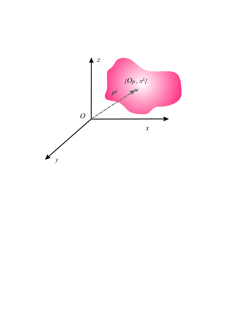
Figure 1: Reference systems for the overall solid $\left\{O,x^{\lambda}\right\}=\left(\left\{{\rm x,\;y,\;z}\right\}\right)\}$ and for each point $p$ in it $\left\{O_{p},x^{\lambda}\right\}=\left(\left\{{\rm x,\;y,\;z}\right\}\right)\}$. Each point has an associated Cauchy tensor acting on it (see Figure 2).

At microscopic level, the plasticity in a solid is produced by a set of slips, generated by the movement of dislocations, defects, etc [19]. The stress acting on the solid is the generator of these slips. We want to take into account all these microscopic dynamical processes at the macroscopic scale. So the theory is based on the decomposition of a solid material into parts as macroscopic points p (Figure 1). These macroscopic points do not need to have any physical reality (grains or others), but points have macroscopic information about microscopic dynamical processes. This macroscopic information is purely statistical, so a macroscopic point is a statistical concept that takes into account all the microscopic information inside it. The set of slips inside a macroscopic point induces the irreversible macroscopic movement of this point (with a well determined spatial directionality). The global movements of the points result in macroscopic plasticity that follow macroscopic laws (theory postulates). So, the proposed unified theory examines plasticity at each macroscopic point p in a solid. The plasticity of the macroscopic points are described by orthogonal transformation groups (directionality of plasticity) acting on Cauchy tensor (generator of plasticity) in a convex manner (measure of plasticity).

The macroscopic anisotropy description by coordinate tensors appears in the infinitesimal orthogonal transformation of Cauchy stress tensor (which acts on the solid point) with respect to a reference system (for the solid point). The directions of these infinitesimal transformations are limited only by the internal structure (microscopic dynamic processes) of macroscopic solid points. These directions of transformation (anisotropy characterization) are described by the coordinate tensors (parameters that depend on the internal variables). A measure (mathematical norm) of the infinitesimal orthogonal transformation of Cauchy tensor gives the macroscopic effect of plasticity (plasticity function). The ensuing point information can be used to obtain a global points statistic for the whole solid.

Certain approaches are considered in this theory. The potential effects of temperature and strain are ignored (temperature-independent and rate-independent plasticity), and so is the time-dependence of all parameters and variables since the only target is critical plasticity in the solid (time-independent plasticity). Our theory relies on the following three postulates:

1. First postulate: the macroscopic units or points that become plastic in a solid are described by second-order Cauchy tensors.

2. Second postulate: hydrostatic-pressure independent plasticity acts at every point in the Tangent Space to the Cauchy Tensor (TSCT). Any type of plasticity at least needs a component in this space TSCT.

3. Third postulate: the plasticity function is convex in the stress space.

Within the framework of the proposed theory, solids are represented in a three-dimensional Euclidean space $E\eqref{GrindEQ__3_}$ where each point or neighbourhood $p\in E\eqref{GrindEQ__3_}$ is defined by the pair $p\equiv\{p^{\lambda},\sigma^{kl}\}\in E\eqref{GrindEQ__3_}$, with indices $\lambda,k,l=x,y,z$. The set of points is referred to $E\eqref{GrindEQ__3_}$ via a coordinate system or reference system $\{O,x^{\lambda}=(x,y,z)\}$ that is shared by the whole solid; the coordinate system has $O$ as its origin and $x^{\lambda}=(x,y,z)$ as its axes. Therefore, a point p in the solid lies at $p^{\lambda}$ in the reference system and has the symmetric second-order stress tensor or Cauchy tensor acting on it, i.e., $\sigma\equiv\sigma^{kl}$ (first postulate); this postulate is valid only for solids with “near-action” internal forces [24]. Since the solid is examined point-wise, each point p possesses its own reference system, $\{O_{p},x^{\lambda}=\left({\rm x,\;y,\;z}\right)\}$, with its origin at $p^{\lambda}$ and $x^{\lambda}=\left({\rm x,\;y,\;z}\right)$ as axes. So the set of stresses acting on the points in the solid define a 2-tensor stress field in the space $E\eqref{GrindEQ__3_}$, which endows the solid with geometric structure (Figure 1).

The reference system for each point, $\{O_{p},x^{\lambda}=\left({\rm x,\;y,\;z}\right)\}$, is arbitrary only when the ensuing equations are invariant under a reference system change (tensor equations), that is, independent of the particular reference system. From the geometric point of view this guarantees that the tensor equations that describe the solid contain, codified as geometric information, all the physical behaviour throughout the directions of reference system changes for the corresponding space.

If the Cauchy tensor is invariant under a change in the origin and axes over the solid, $\{O_{p_{1}},x^{\lambda}=(x,y,z)\}\to\{O_{p_{2}},\bar{x}^{\lambda}={\rm(}\bar{x},\bar{y},\bar{z}{\rm)}\}$, then the solid is stress-homogeneous. If the Cauchy tensor is invariant under a change in the axes directions, $\{O_{p},x^{\lambda}=(x,y,z)\}\to\{O_{p},\bar{x}^{\lambda}={\rm(}\bar{x},\bar{y},\bar{z}{\rm)}\}$, then the stresses at the point p in the solid are isotropic. The degree of homogeneity in the solid can be assessed by examining it point-wise and using the results to develop a global statistics for the entire solid. In this work, we will assume the behaviour of the solid is similar to its individual points or, in other words, that examining a single point will be the same as studying the entire solid.

The intrinsic properties of the solid at each point are examined via a series of transformations with a fixed origin on it. A transformation of the Cauchy tensor, $\sigma^{kl}$, at point p can be interpreted in two completely equivalent ways. In the first one, the reference system ${\rm x}^{\lambda}$ has the Cauchy tensor $\sigma^{kl}$; therefore, a transformation ${\rm x}^{\lambda}\to\bar{{\rm x}}^{\lambda}$ in the reference system will lead to a new reference system $\bar{{\rm x}}^{\lambda}$ with a Cauchy tensor $\bar{\sigma}^{ij}$; this constitutes a reference system transformation or active transformation. In the other interpretation, the reference system ${\rm x}^{\lambda}$ remains unchanged and the Cauchy tensor transformation, $\sigma^{kl}\to\bar{\sigma}^{ij}$, produces a new tensor that is expressed (oriented) in the reference system $\bar{{\rm x}}^{\lambda}$; this is a Cauchy tensor transformation or passive transformation. These two interpretations are mutually related by a negative sign.

The proposed theory relies on a continuous linear transformation of the stress at each point p represented by the tensor $A^{ij}_{kl}$. Such a transformation does not alter the origin of p, which is defined by the coordinates $p^{\lambda}$, but only its coordinate axes, $x^{\lambda}$. Thus, the transformation operator $A^{ij}_{kl}$ acts on the stress tensor $\sigma^{kl}$ to give the transformed tensor $\bar{\sigma}^{ij}$ in accordance with the following expression:

$$A^{ij}_{kl}\sigma^{kl}=\bar{\sigma}^{ij}$$ (21)

where the multilinear transformation $A^{ij}_{kl}$ is a 4-tensor of indices $i,j,k,l=x,y,z$ with two covariant $(k,l)$ and two contravariant$(i,j)$ indices. Mathematically, it follows that this expression is a tensor equation (i.e., that it is invariant under a coordinate system change). Since the resulting transformed tensor, $\bar{\sigma}^{ij}$, has a fixed origin (the same that $\sigma^{kl}$), the transformation can be tangent or normal to the tensor $\sigma^{kl}$. In the former case, it will produce rotations and/or reflections of use for studying anisotropy; in the latter case, it will result in dilatation or dilatation–reflection useful with a view to examining hydrostatic pressure-dependence.

The plasticity at a point p under the influence of an arbitrary initial Cauchy tensor depends on the tangent and normal spaces to the Cauchy tensor. These spaces arise directly from the geometric generalization of the two types of components of the Cauchy tensor. The direct sum of the tangent and normal spaces constitutes the overall stress space at the point concerned. As implied by our second postulate, a solid will yield plasticity at a given point only if a component on the tangent space exists at such a point. As a result, plasticity starts in the associated pure tangent space (hydrostatic-pressure independent plasticity) or, in other words, it never starts in the associated pure normal (hydrostatic-pressure dependent plasticity) space. In fact, there is solid experimental evidence that plasticity never arises under conditions of pure hydrostatic pressure [4, 26]. Thus, some solids exhibit slight elastic (reversible) deformation rather than plasticity, even at very high pure compressive hydrostatic pressures. However, high stress-induced hydrostatic pressures in a solid under tension can lead to an unexpected spatial stress concentration eventually leading to fragile fracture [5, 6].

5 Rotational transformation of the Cauchy tensor

Properly examining plasticity in a solid entails starting in the Tangent Space to the Cauchy Tensor (TSCT) associated to each point p in the solid, and applying a pure orthogonal transformation $R^{ij}_{kl}$ such that

$$R^{ij}_{kl}\sigma^{kl}=\bar{\sigma}^{ij},$$ (22)

where the orthogonality condition is described by means of the matrix equation $R^{T}R=I$. Based on this tensor equation, the Cauchy tensor $\sigma^{kl}$ associated to each point p in the solid is rotated by $R^{ij}_{kl}$ according to a given parameter, which provides the new associated tensor $\bar{\sigma}^{ij}$, which will be the new associated tensor acting on p. Stress rotations according to equation (22) provide a point-wise definition of hydrostatic-pressure independent plasticity in the solid. In this sense, rotations of the Cauchy tensor at p can be interpreted physically as due to some tangential stresses acting on the point. In this respect, the hydrostatic-pressure independent plasticity interaction (i.e., that having no hydrostatic component) is fully defined by the rotations $R^{ij}_{kl}$ and their associated transformation parameters.

The orthogonal rotation transformation $R^{ij}_{kl}$ is a three-dimensional 4-tensor (i.e., one with $3^{4}=81$ components) equivalent to a Mohr transformation if parameterized in Euler angles $\Theta_{E}=\Theta_{E}(\alpha,\beta,\gamma)$ [27]. As noted earlier, the orthogonal rotation transformation is necessary for hydrostatic-pressure independent plasticity to develop at individual points in a solid. However, additional, non-orthogonal transformations (e.g., dilations) can also be applied that will alter the hydrostatic-pressure independent plasticity conditions imposed by a rotation (see Section 11). The remainder of this section, and all subsequent ones up to the eleventh, is devoted to examine hydrostatic-pressure independent plasticity as defined in eq. (22). Section 11 is concerned with hydrostatic pressure-dependence.

The transformation equation (22) connects geometric objects via double indices (i.e., 9 components). However, an equivalent representation connecting objects via single indices (i.e., 3 components) can be obtained by using the following relations:

$$\bar{u}^{i}=R^{i}_{j}u^{j};\quad\quad u^{j}=R^{j}_{i}\bar{u}^{i}$$ (23)

$$u^{j}=T^{jq}v_{q};\quad\quad\bar{u}^{j}=T^{jq}\bar{v}_{q}$$ (24)

where (23) defines the rotational transformations of contravariant vectors and (24) the general contravariant transformations for a vector under coordinate system changes (i.e., the definition of a 1-tensor). From the rotational transformation (23) and general coordinate transformation (24) for each 1-tensor, one can obtain

$$\left.\begin{array}[]{l}{\bar{u}^{i}=R^{i}_{j}u^{j}=R^{i}_{j}T^{jq}v_{q}=R^{i}_{j}T^{jq}R_{q}^{p}\bar{v}_{p}}\\ {\bar{u}^{i}=\bar{T}^{ip}\bar{v}_{p}}\end{array}\right\}\Rightarrow\bar{T}^{ip}=R^{i}_{j}T^{jq}R_{q}^{p}$$ (25)

Since the coordinate system change occurs via the stress 2-tensor (Cauchy tensor) $T^{jq}\equiv\sigma^{jq}$, we can express the transformation by means of a rotational operator

$$\bar{\sigma}^{ij}=R^{i}_{k}\sigma^{kl}R_{l}^{j}\Leftrightarrow\bar{\sigma}=R^{T}\sigma R,$$ (26)

the latter describing the transformation rule for the Cauchy tensor. It is straightforward to verify that this expression is equivalent to (22). The 2-tensor rotations of the types $R^{i}_{k}$ and $R{}_{l}^{j}$can be adequately realized in terms of 3 $\times$ 3 matrices. Relation (26) is invariant under a general change of the coordinate system.

Therefore, the transformations$R^{i}_{k}$, $R{}_{l}^{j}$ lead the plastic process at each point p in the solid. Their study is facilitated by considering the three-dimensional special orthogonal group $SO\eqref{GrindEQ__3_}$ of rotations in the three-dimensional Euclidean space $E\eqref{GrindEQ__3_}$. The main advantage of this approach is that $SO\eqref{GrindEQ__3_}$ possesses both the structure of a group of transformations and a differentiable manifold, which enables us to confer additional invariance properties to the tensor operators defined over it [12].

The elements of the special orthogonal group $SO\eqref{GrindEQ__3_}$ are the orthogonal transformations of the Euclidean space $E\eqref{GrindEQ__3_}$ that describe orientation and length preserving movements. Such rotations are usually represented by orthogonal real 3 $\times$ 3 matrices $R^{T}R=I$ with unit determinant $(\det R=+1)$, and the group product operation is the usual matrix multiplication. Topologically, $SO\eqref{GrindEQ__3_}$ is a compact, non-simply connected group [30]. As Lie group, $SO\eqref{GrindEQ__3_}$ is simple, i.e., the only normal subgroups it contains are the trivial ones: itself and the identity group. In particular, its Lie algebra $so\eqref{GrindEQ__3_}$, which coincides with the tangent space at the identity element, is also a simple Lie algebra. As a consequence of the Lie structure the tangent bundle $TSO\eqref{GrindEQ__3_}\equiv\bigcup_{\rho^{\nu}\in SO\eqref{GrindEQ__3_}}TSO\eqref{GrindEQ__3_}_{\rho^{\nu}}$ inherits special properties that will be useful in our later analysis.

6 Action of the group SO(3) on the Cauchy tensor

Using the adjoint representation of $SO\eqref{GrindEQ__3_}$, the action of the rotations $R^{ij}_{kl}$ in (22) or the equivalent pair $R^{i}_{k}$, $R{}_{l}^{j}$ in (26) can be explicitly expressed in terms of the Euler angles $\Theta_{E}=\Theta_{E}(\alpha,\beta,\gamma)$ as:

$$\left\{\begin{array}[]{l}{\bar{\sigma}^{xx}=\sigma^{xx}\cos^{2}\gamma+\sigma^{yy}sin^{2}\gamma+2\sigma^{xy}sin\gamma\cos\gamma}\\ {\bar{\sigma}^{yy}=\sigma^{yy}\cos^{2}\gamma+\sigma^{xx}sin^{2}\gamma-2\sigma^{xy}sin\gamma\cos\gamma}\\ {\bar{\sigma}^{zz}=\sigma^{zz}}\\ {\bar{\sigma}^{xy}=\sigma^{xy}(\cos^{2}\gamma-sin^{2}\gamma)+(\sigma^{yy}-\sigma^{xx})sin\gamma\cos\gamma}\\ {\bar{\sigma}^{yz}=\sigma^{yz}\cos\gamma-\sigma^{xz}sin\gamma}\\ {\bar{\sigma}^{xz}=\sigma^{yz}sin\gamma+\sigma^{xz}\cos\gamma}\end{array}\right.\begin{array}[]{l}{}\\ {}\end{array}$$ (27)

$$\left\{\begin{array}[]{l}{\bar{\sigma}^{xx}=\sigma^{xx}\cos^{2}\beta+\sigma^{zz}sin^{2}\beta+2\sigma^{xz}sin\beta\cos\beta}\\ {\bar{\sigma}^{yy}=\sigma^{yy}}\\ {\bar{\sigma}^{zz}=\sigma^{zz}\cos^{2}\beta+\sigma^{xx}sin^{2}\beta-2\sigma^{xz}sin\beta\cos\beta}\\ {\bar{\sigma}^{xy}=\sigma^{yz}sin\beta+\sigma^{xy}\cos\beta}\\ {\bar{\sigma}^{yz}=\sigma^{yz}\cos\beta-\sigma^{xy}sin\beta}\\ {\bar{\sigma}^{xz}=\sigma^{xz}(\cos^{2}\beta-sin^{2}\beta)+(\sigma^{zz}-\sigma^{xx})sin\beta\cos\beta}\end{array}\right.\begin{array}[]{l}{}\\ {}\end{array}$$ (28)

$$\left\{\begin{array}[]{l}{\bar{\sigma}^{xx}=\sigma^{xx}}\\ {\bar{\sigma}^{yy}=\sigma^{yy}\cos^{2}\alpha+\sigma^{zz}sin^{2}\alpha-2\sigma^{yz}sin\alpha\cos\alpha}\\ {\bar{\sigma}^{zz}=\sigma^{zz}\cos^{2}\alpha+\sigma^{yy}sin^{2}\alpha+2\sigma^{yz}sin\alpha\cos\alpha}\\ {\bar{\sigma}^{xy}=\sigma^{xy}\cos\alpha-\sigma^{xz}sin\alpha}\\ {\bar{\sigma}^{yz}=\sigma^{yz}(\cos^{2}\alpha-sin^{2}\alpha)+(\sigma^{yy}-\sigma^{zz})sin\alpha\cos\alpha}\\ {\bar{\sigma}^{xz}=\sigma^{xy}sin\alpha+\sigma^{xz}\cos\alpha}\end{array}\right.$$ (29)

A rotation at the point p therefore represents a transformation from the reference system ${\rm\{O}_{{\rm p}}{\rm,x}^{\lambda}\}$, with a tensor $\sigma^{kl}$, to the new reference system ${\rm\{O}_{{\rm p}}{\rm,}\bar{{\rm x}}^{\lambda}\}$, with associated tensor $\bar{\sigma}^{ij}$. The components of the Cauchy tensor in the rotated reference system $\bar{\sigma}^{ij}$ are expressed in terms of $\sigma^{kl}$ by means of equations (27) - (29).

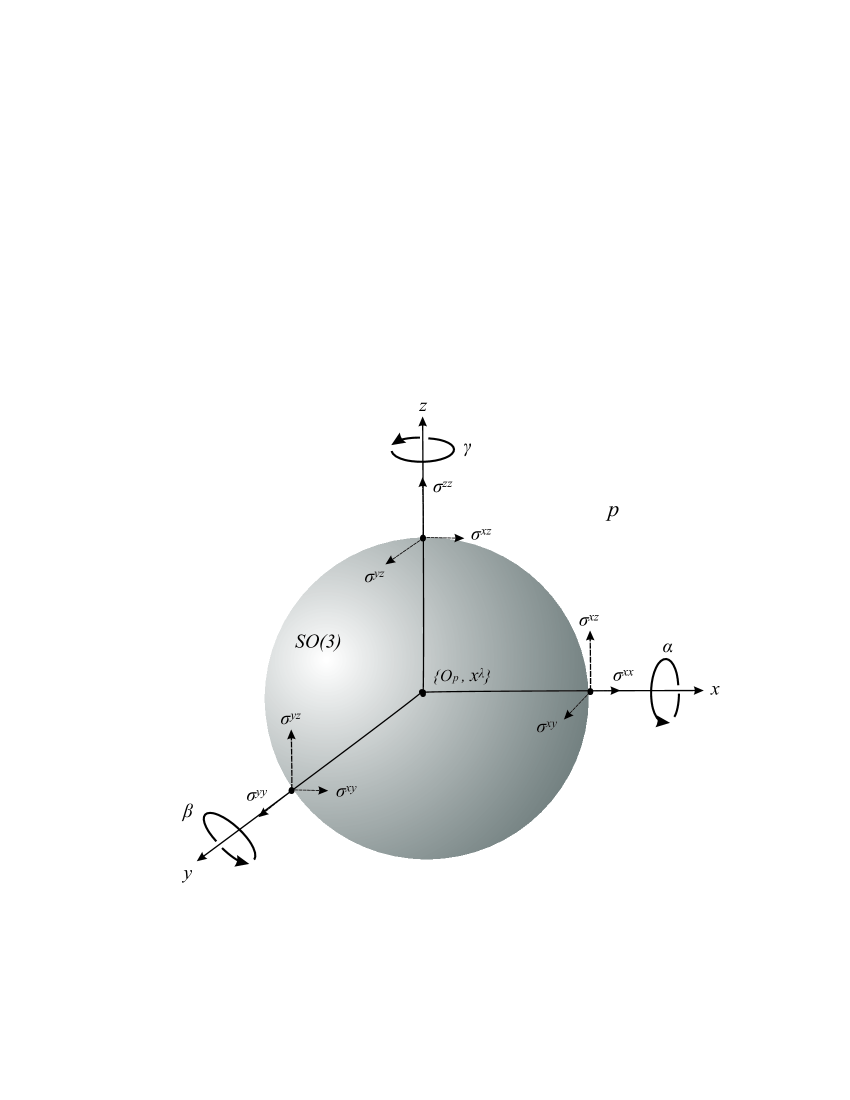
Figure 2: Representation of the Cauchy tensor $\sigma^{kl}$ and its rotational possibilities about the Euler angles $\Theta_{E}=\Theta_{E}(\alpha,\beta,\gamma)$ in the reference system ${\rm\{O}_{{\rm p}}{\rm,x}^{\lambda}\}$. The sphere surface in the figure is a particular making of the $SO\eqref{GrindEQ_3_}$ rotation group.

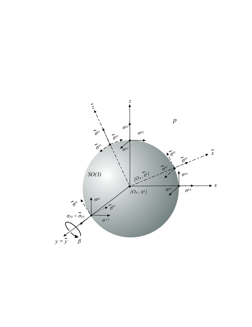
Figure 3: Action of the $SO\eqref{GrindEQ__3_}$ rotation group on the Cauchy tensor $\sigma^{kl}$ for a partial rotation $\beta$ about the $y$-axis, represented by the reference system transformation ${\rm\{O}_{{\rm p}}{\rm,x}^{\lambda}\}\to{\rm\{O}_{{\rm p}}{\rm,}\bar{{\rm x}}^{\lambda}\}$.

The rotation by angle $\Theta_{E}=\Theta_{E}(\alpha,\beta,\gamma)$ can be easily visualized by viewing the reference system in the direction from the positive ends of the axes to their origin and rotating $x^{\lambda}$ anti-clockwise to the new system, $\bar{x}^{\lambda}$, by an angle $\alpha$, $\beta$ and $\gamma$ about the x, y and z axis, respectively (see Figures 2 and 3). Obviously, because of the non-Abelianity of $SO\eqref{GrindEQ__3_}$, the order in which the three partial rotations are performed strongly influences the general rotational outcome.

The action of a generic rotation on the Cauchy tensor is the result of applying successive partial rotations (Figure 3) about each axis in a given sequence. Thus, applying the rotations following the sequence $\alpha\to\beta\to\gamma$, we get

$$\bar{\sigma}^{ij}=R^{ij}_{kl}(\Theta_{E})\sigma^{kl}=R^{ij}_{kl}(\gamma,\beta,\alpha)\sigma^{kl}$$ (30)

which is equivalent to the following expression for rotations in the group $SO\eqref{GrindEQ__3_}$:

$$\bar{\sigma}^{ij}=[R(\gamma)R(\beta)R(\alpha)]^{i}_{k}\sigma^{kl}[R(\alpha)R(\beta)R(\gamma)]_{l}^{j}\Leftrightarrow\bar{\sigma}=R^{T}(\gamma,\beta,\alpha)\sigma R(\alpha,\beta,\gamma)$$ (31)

with partial rotations performed following the sequence $\alpha\to\beta\to\gamma$. We observe that, although equations (27) - (29) depend on the explicit choice of rotation parameters, the transformation does not alter the form of equations (30) and (31), which, as noted earlier, are invariant under a change of coordinate system.

7 Infinitesimal action of SO(3) on the Cauchy tensor

Because of the properties of Lie algebras and the local diffeormorphism on a neighbourhood of the identity element [12], the action (31) on the Cauchy tensor can be also described in terms of the infinitesimal rotations, which turn out to be the generators of $so\eqref{GrindEQ__3_}$.

The Lie group $SO\eqref{GrindEQ__3_}$ and its associated Lie algebra, $so\eqref{GrindEQ__3_}$, are related via the exponential mapping. Given an element $X_{\nu}\in so\eqref{GrindEQ__3_}$, the exponential map provides an element of $SO\eqref{GrindEQ__3_}$ by means of the relation:

$$Exp(X_{\nu})=R(\theta^{\nu})=e^{\theta^{\nu}X_{\nu}}.$$ (32)

Since $SO\eqref{GrindEQ__3_}$ is a compact group, it is ensured that Exp is a surjective mapping [30]. Differentiation with respect to the parameter and evaluation at the identity element provides the operator $X$:

$$\begin{array}[]{c}{\left.\frac{\partial}{\partial\theta^{\nu}}R(\theta^{\nu})\right|_{\theta^{\nu}=0}=X_{\nu}}\\ {\left.\frac{d}{d\Theta}R(\Theta_{E})\right|_{\Theta=0}=\rho^{\nu}\left.\frac{\partial}{\partial\theta^{\nu}}R(\theta^{\nu})\right|_{\theta^{\nu}=0}=\rho^{\nu}X_{\nu}=X}\end{array}$$ (33)

The operators $X$ in the Lie algebra therefore correspond to infinitesimal rotations and can be expressed as linear combinations of the operators for the local basis $X_{\nu}\equiv\partial/\partial\theta^{\nu}$ in the Lie algebra $so\eqref{GrindEQ__3_}$. As a result, each infinitesimal rotation can be expressed as $X=\rho^{\nu}X_{\nu}\equiv\rho^{\nu}\left(\partial/\partial\theta^{\nu}\right)$, which has $\rho^{\nu}$ as its local coordinates.

The actions of infinitesimal rotations on the stress field are determined by the exponential map (32), which relates the group and the Lie algebra; this equation is a function of the infinitesimal generators $X_{\nu}$ of each partial rotation. A first-order series expansion about the angle $\theta^{\nu}=0$ (group identity) yields the expression:

$$R(\theta^{\nu})=e^{\theta^{\nu}X_{\nu}}=I+X_{\nu}\delta\theta^{\nu}+...$$ (34)

where $\Theta_{E}=\Theta_{E}(\alpha,\beta,\gamma)\equiv\Theta_{E}(\theta^{1},\theta^{2},\theta^{3})$ denote the Euler angles associated to the first-order infinitesimal rotations $\delta\theta^{\nu}$, which can take the values $\delta\theta^{\nu}=\delta\alpha,\delta\beta,\delta\gamma$. In addition, each infinitesimal angle $\delta\theta^{\nu}$ has an associated infinitesimal generator $X_{\nu}\equiv\partial/\partial\theta^{\nu}$. Substituting (34) into the rotational expression for a 2-tensor [eq. (31)] yields the expression describing the action of partial infinitesimal rotations, by an angle $\theta^{\nu}$, on the Cauchy tensor. For a first-order approximation, such an expression is of the form

$$\begin{array}[]{l}{\sigma(\theta^{\nu}+\delta\theta^{\nu})=\left(I+X_{\nu}\delta\theta^{\nu}\right)^{T}\sigma(\theta^{\nu})\left(I+X_{\nu}\delta\theta^{\nu}\right)=}\\ {\;\;\;\;\;\;\quad\;\quad\quad\;=\sigma(\theta^{\nu})+\{\sigma(\theta^{\nu})X_{\nu}+X_{\nu}^{T}\sigma(\theta^{\nu})\}\delta\theta^{\nu}+O^{2}\left(\delta\theta^{\nu}\right)}\end{array}$$ (35)

where eq. (31) has been applied on the assumption that $\bar{\sigma}=\sigma(\theta^{\nu}+\delta\theta^{\nu})$ and $\sigma=\sigma(\theta^{\nu})$ (i.e., the neither the origin nor the rotation centre of the tensor is altered, since the transformation of the Cauchy tensor involves rotations only, so that the tensor remains unchanged but is evaluated at a different angle). Equation (35) can be used to establish the first-order variation at each partial angle, which is of the form

$$\begin{array}[]{c}{\sigma(\theta^{\nu}+\delta\theta^{\nu})-\sigma(\theta^{\nu})=\sigma(\theta^{\nu})X_{\nu}\delta\theta^{\nu}+\left(X_{\nu}\right)^{T}\sigma(\theta^{\nu})\delta\theta^{\nu}\Leftrightarrow}\\ {\Leftrightarrow\frac{\delta\sigma}{\delta\theta^{\nu}}=\sigma X_{\nu}+\left(X_{\nu}\right)^{T}\sigma=[\sigma,X_{\nu}]}\end{array}$$ (36)

where the infinitesimal generators $X_{\nu}$ for $SO\eqref{GrindEQ__3_}$ are antisymmetric and the binary operation $[\sigma,X_{\nu}]=\sigma X_{\nu}-X_{\nu}\sigma$ is the commutator between the stress field and the infinitesimal generators $X_{\nu}$. Equation (36) is a function of the specific basis $X_{\nu}$ associated to the Euler angles. Expressing it in terms of an invariant generic infinitesimal rotation $X$ describing the tangent spaces to $SO\eqref{GrindEQ__3_}$ in any arbitrary coordinate system entails introducing the local coordinates $\rho^{\nu}$ associated to the local basis $X_{\nu}$ for the infinitesimal rotation $X$.

This results in a first-order variation of the tensor stress field $\sigma$ with the invariant generator (infinitesimal rotation) $X=\rho^{\nu}X_{\nu}$ of the form

$$\left.d\sigma\right|_{1}\equiv[\sigma,X]=\sigma X-X\sigma=\rho^{\nu}\frac{\delta\sigma}{\delta\theta^{\nu}}$$ (37)

which is the equation for a 2-tensor. Since the operator $X$ is antisymmetric, then $\left.d\sigma\right|_{1}\equiv[\sigma,X]=-[X,\sigma]\equiv-\left.dX\right|_{1}$, based on which the variation of $\sigma$ with $X$ is equivalent to that of $X$ with $\sigma$ with the opposite sign. This is consistent with the two interpretations of a transformation provided in Section 4 as applied to a first-order variation.

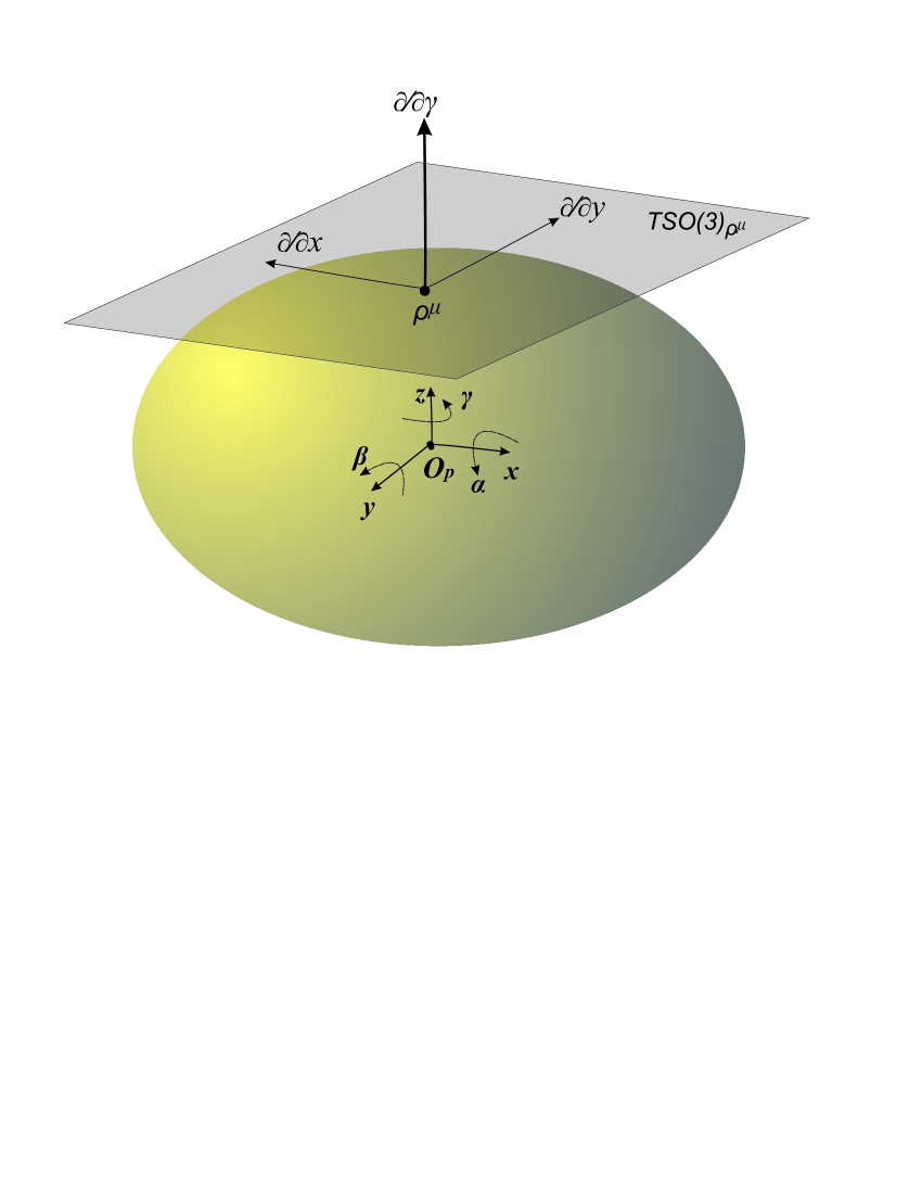
Figure 4: Arbitrary representation of TSCT as an ellipsoid. The tangent space $TSO\eqref{GrindEQ__3_}_{\rho^{\mu}}$ that provides a first-order approximation of TSCT to a reduced neighbourhood of $\rho^{\mu}$ is shown.

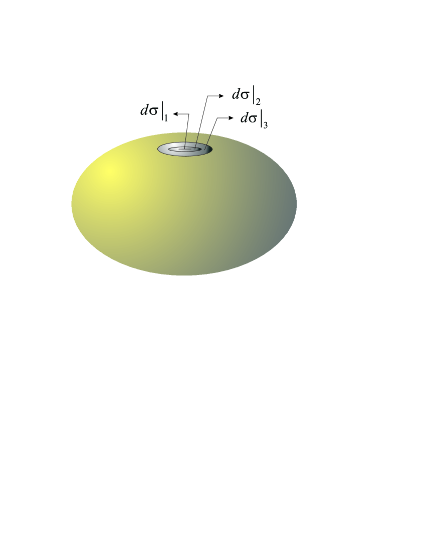
Figure 5: Arbitrary representation of TSCT and its approximations of different order to an infinitesimal neighbourhood. The higher orders lead to local infinitesimal neighbourhood that provide a more accurate description of the overall structure of TSCT.

The tangent space produced by the first-order variation (37) is a linear combination of Euler angles (or, similarly, generators $X_{\nu}$) where each term is linearly dependent on the angles (or generators); therefore, eq. (37) comprises a linear basis of generators $X_{\nu}$ (an Euclidean space). This linear approximation describes TSCT at a first-order local level only (i.e., in very small or local neighbourhoods) (see Figure 4). Expanding such neighbourhoods entails using higher-order approximations involving non-linear combinations in the $X_{\nu}$ generator basis (i.e., non-Euclidean spaces for the different orders) (Figure 5). As shown below by explicit calculations, all spaces approximating TSCT are traceless (i.e., the complete approximation are in fact tangent to the Cauchy tensor). This allows TSCT to be described by means of expansion series of different order.

If one assumes anisotropy at each point in a solid to be more accurately described by including higher order-terms in the series, then the geometric interpretation of such anisotropy suggests that the more local the space —and the smaller the neighbourhood—, the higher will be the degree of isotropy. The inclusion of terms of an increasingly higher order gradually makes the local structure complex enough to facilitate extension of each infinitesimal neighbourhood, with improves approximation, to the entire TSCT. The complex behaviour of solids as concerning symmetry, anisotropy and various other properties dictates the structure of TSCT and hence the approximation orders needed for an accurate description.

Higher-order variations are calculated by applying eq. (37) recursively or, alternatively, expanding the total rotation in (31) up to the required order.

The second-order variation of the stress field $\sigma$ with the rotation $X=\rho^{\nu}X_{\nu}$ can thus be expressed as the following symmetric 2-tensor:

$$\left.d\sigma\right|_{2}\equiv[[\sigma,X],X]=\sigma XX-2X\sigma X+XX\sigma=\rho^{\nu\mu}\frac{\delta^{2}\sigma}{\delta\theta^{\nu}\delta\theta^{\mu}}$$ (38)

which represents the second-order approximation space with coordinates $\rho^{\nu\mu}=\rho^{\nu}\rho^{\mu}$ in the operator basis $X_{\nu\mu}=X_{\nu}X_{\mu}=\frac{\partial^{2}}{\partial\theta^{\nu}\partial\theta^{\mu}}$, the action of which on $\sigma$ being self-apparent from this expression.

The third-order variation of the stress field $\sigma$ with the rotation $X=\rho^{\nu}X_{\nu}$ can be expressed as the following symmetric 2-tensor:

$$\left.d\sigma\right|_{3}\equiv[[[\sigma,X],X],X]=\sigma XXX-3X\sigma XX+3XX\sigma X-XXX\sigma=\rho^{\nu\mu\omega}\frac{\delta^{3}\sigma}{\delta\theta^{\nu}\delta\theta^{\mu}\delta\theta^{\omega}}$$ (39)

This equation represents the third-order approximation space with coordinates $\rho^{\nu\mu\omega}=\rho^{\nu}\rho^{\mu}\rho^{\omega}$ in the operator basis $X_{\nu\mu\omega}=X_{\nu}X_{\mu}X_{\omega}=\frac{\partial^{3}}{\partial\theta^{\nu}\partial\theta^{\mu}\partial\theta^{\omega}}$, the action of which on $\sigma$ is also straightforward.

Higher order approximations are computed by following the same procedure. As a result one obtains a symmetric n-tensor of coordinates $\rho^{\nu...\kappa}=\rho^{\nu}\cdot...\cdot\rho^{\kappa}$ in the basis $X_{\nu...\kappa}=X_{\nu}\cdot\ldots\cdot X_{\kappa}=\frac{\partial^{n}}{\partial\theta^{\nu}\cdot\ldots\cdot\partial\theta^{\kappa}}$ for each n-order. Also, each n-order variation encompasses a total of $\left(\begin{array}[]{c}{3+n-1}\\ {n}\end{array}\right)$ terms, each of which can be factored into sets of n generators $X_{\nu}$, where the resulting factors represent the basis $X_{\nu...\kappa}$ in the n-order approximation space. Therefore, each n-order is represented by the corresponding coordinates $\rho^{\nu...\kappa}$ in the basis $X_{\nu...\kappa}$, and the coordinates represent a symmetric n-tensor with $\left(\begin{array}[]{c}{3+n-1}\\ {n}\end{array}\right)$ independent components. Note that the n-tensors of coordinates depend on the internal variables, $\rho^{\nu}=\rho^{\nu}(\xi),\;\ldots,\;\rho^{\nu...\kappa}=\rho^{\nu...\kappa}(\xi)$; tensors of coordinates can be properly taken as the position internal variables that describe anisotropy.

Each variation has an equivalent interpretation, whatever its order, since transforming the axes of the reference system is equivalent to transforming the stresses involved —with a negative sign (see Section 4) by virtue of the antisymmetric nature of the Lie bracket.

The infinitesimal generators of $SO\eqref{GrindEQ__3_}$ conform to the following commutation relations:

$$[X_{a},X_{b}]=\varepsilon_{abc}X_{c}$$ (40)

where $\varepsilon_{abc}$ is the Levi–Civita symbol. These generators can be expressed as 2-tensors of the form

$$\begin{array}[]{l}{X_{1}=\frac{\partial}{\partial\alpha}=\left(\begin{array}[]{ccc}{0}&{0}&{0}\\ {0}&{0}&{-1}\\ {0}&{1}&{0}\end{array}\right)}\\ {X_{2}=\frac{\partial}{\partial\beta}=\left(\begin{array}[]{ccc}{0}&{0}&{1}\\ {0}&{0}&{0}\\ {-1}&{0}&{0}\end{array}\right)}\\ {X_{3}=\frac{\partial}{\partial\gamma}=\left(\begin{array}[]{ccc}{0}&{-1}&{0}\\ {1}&{0}&{0}\\ {0}&{0}&{0}\end{array}\right)}\end{array}$$ (41)

In summary, using the three generators of the group $SO\eqref{GrindEQ__3_}$ in eq. (41) in conjunction with the Cauchy tensor $\sigma$ allows us to compute the variation of any order of the Cauchy tensor in order to obtain the different approximation to TSCT.

8 $\mathbf{n}$-Order variations of the stress tensor field

This section specifically examines the variations of different order described in the previous section, which provide different approximations to TSCT.

The first-order variation (37) of $\sigma$ with $X$can be expressed as

$$\begin{array}[c]{l}{[\sigma,X]=\rho^{1}\left(\begin{array}[c]{ccc}{0}&{\sigma_{xz}}&{-\sigma_{xy}}\\ {\sigma_{xz}}&{2\sigma_{yz}}&{\sigma_{zz}-\sigma_{yy}}\\ {-\sigma_{xy}}&{\sigma_{zz}-\sigma_{yy}}&{-2\sigma_{yz}}\end{array}\right)+\rho^{2}\left(\begin{array}[c]{ccc}{-2\sigma_{xz}}&{-\sigma_{yz}}&{\sigma_{xx}-\sigma_{zz}}\\ {-\sigma_{yz}}&{0}&{\sigma_{xy}}\\ {\sigma_{xx}-\sigma_{zz}}&{\sigma_{xy}}&{2\sigma_{xz}}\end{array}\right)+}\\ \quad\quad\quad\quad{\rho^{3}\left(\begin{array}[c]{ccc}{2\sigma_{xy}}&{\sigma_{yy}-\sigma_{xx}}&{\sigma_{yz}}\\ {\sigma_{yy}-\sigma_{xx}}&{-2\sigma_{xy}}&{-\sigma_{xz}}\\ {\sigma_{yz}}&{-\sigma_{xz}}&{0}\end{array}\right)=}\\ {\left(\begin{array}[c]{ccc}{-\rho^{2}2\sigma_{xz}+2\rho^{3}\sigma_{xy}}&{\rho^{1}\sigma_{xz}-\rho^{2}\sigma_{yz}+\rho^{3}(\sigma_{yy}-\sigma_{xx})}&{-\rho^{1}\sigma_{xy}+\rho^{2}(\sigma_{xx}-\sigma_{zz})+\rho^{3}\sigma_{yz}}\\ {\rho^{1}\sigma_{xz}-\rho^{2}\sigma_{yz}+\rho^{3}(\sigma_{yy}-\sigma_{xx})}&{\rho^{1}2\sigma_{yz}-\rho^{3}2\sigma_{xy}}&{\rho^{1}(\sigma_{zz}-\sigma_{yy})+\rho^{2}\sigma_{xy}-\rho^{3}\sigma_{xz}}\\ {-\rho^{1}\sigma_{xy}+\rho^{2}(\sigma_{xx}-\sigma_{zz})+\rho^{3}\sigma_{yz}}&{\rho^{1}(\sigma_{zz}-\sigma_{yy})+\rho^{2}\sigma_{xy}-\rho^{3}\sigma_{xz}}&{-\rho^{1}2\sigma_{yz}+\rho^{2}2\sigma_{xz}}\end{array}\right)}\end{array}$$ (42)

which is a real symmetric traceless 2-tensor parameterized in the coordinates $\rho^{\nu}$. The first-order variation for the particular case of the Cauchy diagonal tensor is

$$[\sigma,X]=\left(\begin{array}[]{ccc}{0}&{\rho^{3}(\sigma_{2}-\sigma_{1})}&{\rho^{2}(\sigma_{1}-\sigma_{3})}\\ {\rho^{3}(\sigma_{2}-\sigma_{1})}&{0}&{\rho^{1}(\sigma_{3}-\sigma_{2})}\\ {\rho^{2}(\sigma_{1}-\sigma_{3})}&{\rho^{1}(\sigma_{3}-\sigma_{2})}&{0}\end{array}\right)$$ (43)

and the second-order variation (38) of $\sigma$ with $X$ is

$$\begin{array}[]{l}{[[\sigma,X],X]^{11}=\rho^{12}2\sigma_{xy}+\rho^{13}2\sigma_{xz}-\rho^{23}4\sigma_{yz}+\rho^{33}2(\sigma_{yy}-\sigma_{xx})+\rho^{22}2(\sigma_{zz}-\sigma_{xx});}\\ {[[\sigma,X],X]^{12}=-(\rho^{11}+\rho^{22}+4\rho^{33})\sigma_{xy}+\rho^{23}3\sigma_{xz}+\rho^{13}3\sigma_{yz}+\rho^{12}(-2\sigma_{zz}+\sigma_{yy}+\sigma_{xx});}\\ {[[\sigma,X],X]^{13}=\rho^{23}3\sigma_{xy}-(\rho^{11}+\rho^{33}+4\rho^{22})\sigma_{xz}+\rho^{12}3\sigma_{yz}+\rho^{13}(-2\sigma_{yy}+\sigma_{xx}+\sigma_{zz});}\\ {[[\sigma,X],X]^{22}=2\rho^{12}\sigma_{xy}-\rho^{13}4\sigma_{xz}+\rho^{23}2\sigma_{yz}-\rho^{33}2(\sigma_{yy}-\sigma_{xx})+\rho^{11}2(\sigma_{zz}-\sigma_{yy});}\\ {[[\sigma,X],X]^{23}=\rho^{13}3\sigma_{xy}+\rho^{12}3\sigma_{xz}+\rho^{23}(-2\sigma_{xx}+\sigma_{yy}+\sigma_{zz})-(4\rho^{11}+\rho^{22}+\rho^{33})\sigma_{yz};}\\ {[[\sigma,X],X]^{33}=-\rho^{12}4\sigma_{xy}+\rho^{13}2\sigma_{xz}+\rho^{23}2\sigma_{yz}-\rho^{22}2(\sigma_{zz}-\sigma_{xx})-\rho^{11}2(\sigma_{zz}-\sigma_{yy})}\end{array}$$ (44)

which is a real symmetric traceless 2-tensor parameterized in the coordinates $\rho^{\nu\mu}=\rho^{\nu}\rho^{\mu}$. The specific expression for the Cauchy diagonal tensor is

$$\left[\left[\sigma,X\right],X\right]=$$

$$\left(\begin{array}[]{ccc}{\rho^{33}2(\sigma_{2}-\sigma_{1})+\rho^{22}2(\sigma_{3}-\sigma_{1})}&{\rho^{12}(-2\sigma_{3}+\sigma_{2}+\sigma_{1}))}&{\rho^{13}(-2\sigma_{2}+\sigma_{1}+\sigma_{3})}\\ {\rho^{12}(-2\sigma_{3}+\sigma_{2}+\sigma_{1})}&{-\rho^{33}2(\sigma_{2}-\sigma_{1})+\rho^{11}2(\sigma_{3}-\sigma_{2})}&{\rho^{23}(-2\sigma_{1}+\sigma_{2}+\sigma_{3})}\\ {\rho^{13}(-2\sigma_{2}+\sigma_{1}+\sigma_{3})}&{\rho^{23}(-2\sigma_{1}+\sigma_{2}+\sigma_{3})}&{-\rho^{22}2(\sigma_{3}-\sigma_{1})-\rho^{11}2(\sigma_{3}-\sigma_{2})}\end{array}\right)$$ (48)

The third-order variation (39) of $\sigma$ with $X$ for the particular case of the Cauchy diagonal tensor is given by:

$$\begin{array}[]{l}{[[[\sigma,X],X],X]^{11}=\rho^{123}6(\sigma_{2}-\sigma_{3});}\\ {[[[\sigma,X],X],X]^{12}=\rho^{333}4(\sigma_{1}-\sigma_{2})+\rho^{223}(4\sigma_{1}-3\sigma_{3}-\sigma_{2})+\rho^{133}(-4\sigma_{2}+3\sigma_{3}+\sigma_{1});}\\ {[[[\sigma,X],X],X]^{13}=\rho^{233}(-4\sigma_{1}+3\sigma_{2}+\sigma_{3})+\rho^{112}(4\sigma_{3}-3\sigma_{2}-\sigma_{1})+\rho^{222}4(\sigma_{3}-\sigma_{1});}\\ {[[[\sigma,X],X],X]^{22}=\rho^{123}6(\sigma_{3}-\sigma_{1});}\\ {[[[\sigma,X],X],X]^{23}=\rho^{133}(4\sigma_{2}-3\sigma_{1}-\sigma_{3})+\rho^{111}4(\sigma_{2}-\sigma_{3})+\rho^{122}(-4\sigma_{3}+3\sigma_{1}+\sigma_{2});}\\ {[[[\sigma,X],X],X]^{33}=\rho^{123}6(\sigma_{1}-\sigma_{2})}\end{array}$$ (49)

which is a real symmetric traceless 2-tensor parameterized in the coordinates $\rho^{\nu\mu\omega}=\rho^{\nu}\rho^{\mu}\rho^{\omega}$.

The following series expansion encompasses those for all variation orders and defines the overall TSCT:

$$d\sigma=\left.d\sigma\right|_{1}+\frac{1}{2!}\left.d\sigma\right|_{2}+\frac{1}{3!}\left.d\sigma\right|_{3}+...=[\sigma,X]+\frac{1}{2!}[[\sigma,X],X]+\frac{1}{3!}[[[\sigma,X],X],X]+.....$$ (50)

Therefore, TSCT is represented by a symmetric traceless 2-tensor (50) that describes hydrostatic-pressure independent plasticity. If the solid concerned is completely isotropic, using the first term in (50) will suffice; if it is orthotropic, the first two will be enough. The plastic processes independent of the hydrostatic pressure are completely characterized by the stress dependences and tensors of coordinates $\rho^{\nu},\ldots,\rho^{\nu\ldots\kappa}$ —in their corresponding bases— in the terms for the different variation orders in (50).

9 The norm space in plastic states

The geometric study of plasticity conducted here involves examining hydrostatic-pressure independent plasticity in the tangent space to the Cauchy tensor (TSCT). As shown above, such a space can be represented by the series expansion (50), which has the typical form for a 2-tensor and gives both the spatial coordinates (degree of anisotropy) in a specific basis and the stress-dependence of hydrostatic-pressure independent plasticity. However, determining the plasticity potential (plasticity interaction) in this situation entails defining a specific metric for the 2-tensor (50). To this extend, expression (50) —or the corresponding partial summation— is used to calculate the scalar norm $g$. The parameters introduced by the definition of the norm are restricted by the constraint that the plasticity function should be convex (third postulate).

Plasticity depends both on the externally applied stresses, $\sigma^{kl}$, and on the intrinsic properties of the material, $\rho^{\nu},\ldots,\rho^{\nu\ldots\kappa}$, in a specific reference system or basis. Therefore, the scalar function $g$ defining the norm will depend on both [i.e., $g=g(\sigma^{kl};\rho^{\nu},...,\rho^{\nu...\kappa})$]. The function $g$ should provide the correlation between multiaxial stresses and hence indicate how the different components of the Cauchy tensor must be related. If $(\sigma^{kl})_{P}$ is defined as the 2-tensor describing the plastic limit of the solid (stress internal variables), then such a limit will be reached when

$$g(\sigma^{kl};\rho^{\nu},...,\rho^{\nu...\kappa})=g((\sigma^{kl})_{P};\rho^{\nu},...,\rho^{\nu...\kappa})$$ (51)

Usually, the tensor $(\sigma^{kl})_{P}$ encompasses a single non-zero uniaxial component and thus coincides with $\sigma_{P}$ (the scalar uniaxial plastic limit that it is an internal variable). This allows the plasticity function to be rewritten as follows:

$$f(\sigma^{kl},(\sigma^{kl})_{P};\rho^{\nu},...,\rho^{\nu...\kappa})=g(\sigma^{kl};\rho^{\nu},...,\rho^{\nu...\kappa})-g((\sigma^{kl})_{P};\rho^{\nu},...,\rho^{\nu...\kappa})$$ (52)

The scalar function $g$ can be defined in terms of a matrix norm $\left\|\cdot\right\|$ such as $L^{m}$ (i.e. the usual m-norm for vectors); therefore,

$$\begin{array}[]{c}{\left\|d\sigma\right\|^{m}\equiv\left(\sum_{i=1}^{3}\sum_{j=1}^{3}\left|d\sigma_{ij}\right|^{m}\right)}\\ {g=\left\|d\sigma\right\|^{m}\Leftrightarrow f=\left\|d\sigma\right\|^{m}-\left\|\left(d\sigma\right)_{P}\right\|^{m}}\end{array}$$ (53)

where the constraints on the norm parameter ($m\in\Re,m\geq 1$) ensure convexity in the plasticity yield criterion (third postulate). The specific value of m depends on the properties of the particular material. Norm (53) can be induced from the scalar product of second-order tensors, which is constructed from the following:

$$<d\sigma,\;d\sigma{{}^{\prime}}>\equiv d\sigma^{kl}d\sigma_{kl}{{}^{\prime}}\stackrel{{\scriptstyle R}}{{\longrightarrow}}<R^{T}d\sigma R,\;R^{T}d\sigma{{}^{\prime}}R>\equiv(R^{i}_{k}d\sigma^{kl}R_{l}^{j})(R_{i}^{k}d\sigma{{}^{\prime}}_{kl}R^{l}_{j})=d\sigma^{kl}d\sigma_{kl}{{}^{\prime}}$$ (54)

This definition, where rotations $R^{i}_{k}$ and $R_{l}^{j}$ are orthogonal $(R^{T}R=I)$, is invariant under rotations (R). The scalar product and its induced norm [eqs (53) and (54)] afford measurement of angles and lengths in TSCT (50).

The definition must be completed with a scalar product of the coordinate tensors at the different independent orders ($\rho^{\nu},\ldots,\rho^{\nu\ldots\kappa}$) of the form

$$\rho^{\nu...\kappa}\rho_{\chi....\xi}=\left(\rho^{\nu}\right)^{2}\cdot....\cdot\left(\rho^{\kappa}\right)^{2}\delta^{\nu}_{\chi}\cdot....\cdot\delta^{\kappa}_{\xi}$$ (55)

The norm induced from this scalar product is $L^{m}$ for the corresponding n-coordinate tensor.

In summary, plasticity yield criteria can be defined by the norms $L^{m}$ induced from the scalar products of stresses (54) and coordinates (55) in the stress and coordinate (position) spaces defined by the series expansion (50). As a result of this construction, the space (50) is normed.

10 Analysis of plasticity yield criteria. Convexity

The norms defined in Section 9 allow one to assess measurements of variations of any order with a view to establishing the plasticity yield criterion for each material in terms of its particular properties.

Isotropic criteria can be analysed by using the norm $L^{m}$ for the first-order variation (42), which gives

$$\begin{array}[]{l}{\left\|\left.d\sigma\right|_{1}\right\|^{m}=2\left|\rho^{3}\right|^{m}\left|\sigma_{yy}-\sigma_{xx}\right|^{m}+2\left|\rho^{1}\right|^{m}\left|\sigma_{zz}-\sigma_{yy}\right|^{m}+2\left|\rho^{2}\right|^{m}\left|\sigma_{xx}-\sigma_{zz}\right|^{m}+}\\ {\quad\quad\quad\quad+\left[2\left|\rho^{1}\right|^{m}+2\left|\rho^{2}\right|^{m}+2^{m+1}\left|\rho^{3}\right|^{m}\right]\left|\sigma_{xy}\right|^{m}+\left[2\left|\rho^{2}\right|^{m}+2\left|\rho^{3}\right|^{m}+2^{m+1}\left|\rho^{1}\right|^{m}\right]\left|\sigma_{yz}\right|^{m}+}\\ {\quad\quad\quad\quad+\left[2\left|\rho^{1}\right|^{m}+2\left|\rho^{3}\right|^{m}+2^{m+1}\left|\rho^{2}\right|^{m}\right]\left|\sigma_{xz}\right|^{m}}\end{array}$$ (56)

With complete spatial isotropy $(\rho^{1}=\rho^{2}=\rho^{3})$ and invariance $(m=2)$, the outcome is the Huber–Von Mises criterion (13). In the particular case of using independent plane stresses $xy,yz,xz$ in each coordinate directions $(0,0,\rho^{3})$, $(\rho^{1},0,0)$, $(0,\rho^{2},0)$ respectively, taking $(m=2)$ and factoring in such a way as to make the criterion smooth (i.e., differentiable) leads to the Tresca criterion (12). With complete spatial isotropy $(\rho^{1}=\rho^{2}=\rho^{3})$, using the Cauchy tensor in principal stress (Cauchy diagonal tensor) gives the Hosford criterion (17). These are the most widely used basic plasticity yield criteria for materials with completely isotropic symmetry.

Anisotropic criteria, which are applicable to orthotropic materials, can be analysed by using the norm $L^{m}$ for the second-order variation (44), which gives

$$\begin{array}[]{l}{\left\|\left.d\sigma\right|_{2}\right\|^{m}=2\left|\rho^{12}\right|^{m}\left|2\sigma_{zz}-\sigma_{xx}-\sigma_{yy}\right|^{m}+2\left|\rho^{13}\right|^{m}\left|2\sigma_{yy}-\sigma_{xx}-\sigma_{zz}\right|^{m}+2\left|\rho^{23}\right|^{m}\left|2\sigma_{xx}-\sigma_{yy}-\sigma_{zz}\right|^{m}+}\\ {\quad\quad\quad+8\left|\rho^{33}\right|^{m}\left|\sigma_{yy}-\sigma_{xx}\right|^{m}+8\left|\rho^{11}\right|^{m}\left|\sigma_{zz}-\sigma_{yy}\right|^{m}+8\left|\rho^{22}\right|^{m}\left|\sigma_{xx}-\sigma_{zz}\right|^{m}+}\\ {\quad\quad\quad+\left[(2+2^{m})\cdot 2^{m}\left|\rho^{12}\right|^{m}+2\cdot 3^{m}\left|\rho^{23}\right|^{m}+2\cdot 3^{m}\left|\rho^{13}\right|^{m}+2\left|\rho^{11}\right|^{m}+2\left|\rho^{22}\right|^{m}+2^{2m+1}\left|\rho^{33}\right|^{m}\right]\left|\sigma_{xy}\right|^{m}+}\\ {\quad\quad\quad+\left[2\cdot 3^{m}\left|\rho^{12}\right|^{m}+(2+2^{m})\cdot 2^{m}\left|\rho^{23}\right|^{m}+2\cdot 3^{m}\left|\rho^{13}\right|^{m}+2^{2m+1}\left|\rho^{11}\right|^{m}+2\left|\rho^{22}\right|^{m}+2\left|\rho^{33}\right|^{m}\right]\left|\sigma_{yz}\right|^{m}+}\\ {\quad\quad\quad+\left[2\cdot 3^{m}\left|\rho^{12}\right|^{m}+2\cdot 3^{m}\left|\rho^{23}\right|^{m}+(2+2^{m})\cdot 2^{m}\left|\rho^{13}\right|^{m}+2\left|\rho^{11}\right|^{m}+2^{2m+1}\left|\rho^{22}\right|^{m}+2\left|\rho^{33}\right|^{m}\right]\left|\sigma_{xz}\right|^{m}}\end{array}$$ (57)

For the particular case of the Cauchy diagonal tensor, this leads to Hill’s second criterion (3). Diagonalizing the coordinate tensor $\rho^{\nu\mu}$ and assuming $(m=2)$, we are led to Hill’s first criterion (14). On the other hand, if both the coordinate tensor, $\rho^{\nu\mu}$, and the Cauchy tensor are diagonalized, then one obtains the Logan–Hosford criterion (18). These criteria hold for anisotropic materials with orthotropic symmetry (i.e., orthotropic materials), a general description of which requires six spatial parameters (the six parameters of the symmetry tensor $\rho^{\nu\mu}$).

The criteria of Barlat et al. [2] and Karafillis & Boyce [22] were originally established by transforming the stress tensor; this involved considering symmetry and anisotropy in the material. Within the framework of the proposed theory, the transformations required to describe these effects in materials can be analysed via transformations of the coordinate tensors $\rho^{\nu},\ldots,\rho^{\nu\ldots\kappa}$ from their starting bases ($X_{\nu},\ldots,X_{\nu....\kappa}$), to those needed for an accurate description of the material concerned. Obviously, anisotropy makes solid materials basis-dependent (i.e., reference system-dependent); therefore, it grows with increasing order of the bases used. In completely isotropic materials, the plasticity yield criterion depends on the coordinates of a single scalar $(\rho^{1}=\rho^{2}=\rho^{3})$, i.e., it is absolutely independent of the particular coordinate system.

In should be noted that Hill’s second criterion, which provides an accurate description of the anomalous behaviour of some materials such as aluminium [18, 37], arises naturally within the framework of the proposed plasticity theory. Additionally, the proposed theory includes the anisotropy criterion of Hosford [25] that can explain the behaviour of fcc (for $m=8$) and bcc (for $m=6$) materials.

With the norms defined above, equation (50) describes the most salient plasticity yield criteria reported so far as particular cases. Therefore, (50) provides a self-contained description of hydrostatic-pressure independent plasticity (i.e., plasticity compliant with the proposed postulates and approximations). A higher-order analysis allows one to establish a generic criterion in terms of the following expanded series:

$$\begin{array}[]{l}{\left\|d\sigma\right\|^{m}=\sum_{n{{}^{\prime}}=0}^{\infty}\sum_{f}u_{n{{}^{\prime}}f}\left|2^{n{{}^{\prime}}}\sigma_{ii}-(2^{n{{}^{\prime}}}-1)\sigma_{jj}-\sigma_{kk}\right|^{m}+v\left|\sigma_{xy}\right|^{m}+w\left|\sigma_{yz}\right|^{m}+k\left|\sigma_{xz}\right|^{m}=}\\ {\quad\quad\quad=\ldots\ldots+u_{a1}\left|2^{a}\sigma_{xx}-(2^{a}-1)\sigma_{yy}-\sigma_{zz}\right|^{m}+u_{a2}\left|2^{a}\sigma_{xx}-(2^{a}-1)\sigma_{zz}-\sigma_{yy}\right|^{m}+}\\ {\quad\quad\quad+u_{a3}\left|2^{a}\sigma_{yy}-(2^{a}-1)\sigma_{xx}-\sigma_{zz}\right|^{m}+u_{a4}\left|2^{a}\sigma_{yy}-(2^{a}-1)\sigma_{zz}-\sigma_{xx}\right|^{m}+}\\ {\quad\quad\quad+u_{a5}\left|2^{a}\sigma_{zz}-(2^{a}-1)\sigma_{xx}-\sigma_{yy}\right|^{m}+u_{a6}\left|2^{a}\sigma_{zz}-(2^{a}-1)\sigma_{yy}-\sigma_{xx}\right|^{m}+}\\ {\quad\quad\quad+\ldots\ldots\ldots\ldots\ldots\ldots\ldots\ldots+u_{21}\left|4\sigma_{xx}-3\sigma_{zz}-\sigma_{yy}\right|^{m}+u_{22}\left|4\sigma_{xx}-3\sigma_{yy}-\sigma_{zz}\right|^{m}+}\\ {\quad\quad\quad+u_{23}\left|4\sigma_{yy}-3\sigma_{zz}-\sigma_{xx}\right|^{m}+u_{24}\left|4\sigma_{yy}-3\sigma_{xx}-\sigma_{zz}\right|^{m}+u_{25}\left|4\sigma_{zz}-3\sigma_{xx}-\sigma_{yy}\right|^{m}+}\\ {\quad\quad\quad+u_{26}\left|4\sigma_{zz}-3\sigma_{yy}-\sigma_{xx}\right|^{m}+u_{11}\left|2\sigma_{zz}-\sigma_{xx}-\sigma_{yy}\right|^{m}+u_{12}\left|2\sigma_{yy}-\sigma_{xx}-\sigma_{zz}\right|^{m}+}\\ {\quad\quad\quad+u_{13}\left|2\sigma_{xx}-\sigma_{yy}-\sigma_{zz}\right|^{m}+u_{01}\left|\sigma_{yy}-\sigma_{xx}\right|^{m}+u_{02}\left|\sigma_{zz}-\sigma_{yy}\right|^{m}+u_{03}\left|\sigma_{xx}-\sigma_{zz}\right|^{m}+}\\ {\quad\quad\quad+v\left|\sigma_{xy}\right|^{m}+w\left|\sigma_{yz}\right|^{m}+k\left|\sigma_{xz}\right|^{m}}\end{array}$$ (58)

where $i\neq j\neq k\neq i$ and the indices can range over $x,y,z$; $f$ is the permutation index. Each term in (58) has an associated coefficient $u_{n{{}^{\prime}}f},v,w,k$ that can be explicitly computed within the framework of the proposed unified theory, but has been excluded in the expanded from (58) for simplicity. Note that positive integer parameter $n=n{{}^{\prime}}+1$ in eq. (58) represents the n-order approximation.

Stress convexity in (58) can be assessed by assuming that a linear combination of convex functions with positive coefficients is a convex function itself [36]. The coefficients $u_{n{{}^{\prime}}f},v,w,k$ are in fact all positive. Therefore, it will suffice to show that the stress-dependence of each individual coefficient in (58) is convex (i.e., that all stresses in the terms $\left|2^{n{{}^{\prime}}}\sigma_{ii}-(2^{n{{}^{\prime}}}-1)\sigma_{jj}-\sigma_{kk}\right|^{m}$, $\left|\sigma_{xy}\right|^{m}$, $\left|\sigma_{yz}\right|^{m}$, $\left|\sigma_{xz}\right|^{m}$ are convex). Convexity in a function T of three variables can be expressed [36] as

$$T(c_{1}\sigma_{ii}+c_{2}\sigma_{jj}+c_{3}\sigma_{kk})\leq c_{1}T(\sigma_{ii})+c_{2}T(\sigma_{jj})+c_{3}T(\sigma_{kk})$$ (59)

where $c_{1},c_{2},c_{3}\in\Re$ are positive or zero and the following condition holds: $c_{1}+c_{2}+c_{3}=1$. The convexity of $\left|\sigma_{xy}\right|^{m}$, $\left|\sigma_{yz}\right|^{m}$, $\left|\sigma_{xz}\right|^{m}$ can be immediately confirmed by applying (59) to the particular case of a single variable. That of $\left|2^{n{{}^{\prime}}}\sigma_{ii}-(2^{n{{}^{\prime}}}-1)\sigma_{jj}-\sigma_{kk}\right|^{m}$ can also be easily inferred from the triangular inequality (see Appendix) fulfilling this $L^{m}$ norm as defined in the stress vector space $(\sigma_{xx},\sigma_{yy},\sigma_{zz})$. Note that, for $L^{m}$ to actually be the norm, $m\in\Re,m\geq 1$, which is the constraint to be imposed on (58) for stresses to be convex. Under these conditions, the plasticity yield criterion (58) will fulfil the third postulate. Within the framework of the proposed theory, the general criterion (58) can predict plastic behaviour in solids. Therefore, it can be of use in future experimental and theory studies on this topic.

11 Hydrostatic pressure-dependent plasticity yield criteria

The hydrostatic pressure-independent definitions obtained in the previous sections invariably include traceless 2-tensors. In fact, this mathematical constraint ensures that the ensuing criteria will be hydrostatic-pressure independent. As noted earlier, the normal space to the Cauchy tensor describes the hydrostatic pressure-dependence of plasticity. As a result, considering the effects of hydrostatic pressure in plasticity yield criteria entails including a $c\left(\sigma_{M}\right)^{b}\equiv c\left(\sigma_{xx}+\sigma_{yy}+\sigma_{zz}\right)^{b}$ dependent function to describe the hydrostatic behaviour of the material with specific coefficients $b,c$ [10, 11, 7, 9]. A more detailed study of the hydrostatic pressure-dependence in the framework of unified theory will be the subject of future work.

12 Conclusions

In this paper we propose a new approach to the theory of macroscopic plasticity, based on a geometrical ansatz, that unifies the different plasticity yield criteria. The method is based on decomposing the Cauchy tensor into its component stress spaces: tangent and normal spaces. Hydrostatic-pressure independent yield criteria are located on the tangent space to the Cauchy tensor (TSCT), whereas hydrostatic-pressure dependent yield criteria are located on the tangent and normal spaces to the Cauchy tensor (TSCT and NSCT). The analysis of the corresponding spaces requires the use of Lie groups of transformations.

This work focuses on the tangent space to Cauchy tensor (TSCT) and analyzes the hydrostatic-pressure independent yield criteria as orthogonal transformations. The measure of this tangent space is taken as a mathematical norm that guarantees the convexity of the yield criteria. From this measure we obtained the convex-stress dependence for both isotropic yield criteria (Tresca 1864 and Von Mises 1913) and anisotropic yield criteria (Hill 1948 and Hill 1979). In addition, a stress series expansion is obtained that allows a detailed study of the mechanical properties in materials: anisotropy, hardening-softening, etc. The tensor coefficients resulting from orthogonal transformations are dependent on internal variables. These tensor coefficients allow a deep analysis of mechanical properties in materials. This unified theory simplifies the great existing amount of yield criteria and gives a physical meaning to the anisotropy coefficients.

This unified theory also allows an analytical study of anisotropy (dependency of $f$on $\xi$) and hardening-softening (dependency of $\dot{f}$ on $\xi$) by means of a set of tensor coefficients. These coefficients are the directions of macroscopic plasticity (by points) in materials. A connection is suggested between macroscopic transformations (unified theory) and the microscopic processes (dislocation theory). To this extent, the concept of macroscopic point, that constitutes a statistical measure of microscopic processes, is introduced. The concept of the point connects two scales with different physical laws.

This unified approach has a series of advantages. At first, it proposes the stress dependencies of yield criteria, starting from very simple postulates and with a unified vision of the underlying phenomena. Further, it allows to know the macroscopic plasticity directions in the solid points, by tensor coefficients of orthogonal transformations. It also provides a manner to analyze the anisotropy and hardening-softening in materials. Finally, it enables us to establish a connection between microscopic plasticity and macroscopic plasticity.

In future work it is important to extend the unified theory to treat the very important question about the hydrostatic pressure-dependent plasticity (important in composites and granular materials); for this it is necessary to analyse dilatation transformations. In this context, it is of fundamental importance to make a deep study of hardening-softening and the time-evolution of plasticity in materials; for the latter aspect it is necessary to determine an adequate time-transformation that gives a correct parameterization of the solid time-evolution.

Notation

(a) Indices

1. Solid point position: $\lambda$ ranging over $x,y,z$

2. Cauchy tensor: $i,j,k,l,p,q$ ranging over $x,y,z$

3. Rotation group: $\nu,\mu,\omega,\kappa,\chi,\xi$ ranging over $1,2,3$

4. Levi–Civita tensor: $a,b,c$ ranging over $1,2,3$

5. Elastic–plastic limit: P

6. Angle equivalence: $(\theta^{1},\theta^{2},\theta^{3})\equiv(\alpha,\beta,\gamma)$

7. Cauchy tensor equivalence: $\sigma\equiv\sigma^{kl}$ (contravariant); $\sigma\equiv\sigma_{kl}$ (covariant)

8. Principal stresses of the Cauchy tensor: $\sigma_{1},\sigma_{2},\sigma_{3}$

9. Hydrostatic pressure: $\sigma_{M}$

10. Internal variables: $\xi=\xi_{\alpha}$

(b) Tensors

The Einstein summation convention is used throughout. Covariant tensor notation is systematically employed from Section 4 onwards.

Acknowledgements.

The first author, José Miguel Luque Raigón, is grateful to Professor Alfredo Navarro of the University of Seville for his helpful, inspiring comments on materials mechanics and plasticity, and also to the members of the Mechanical Engineering and Materials Research Group of the University of Seville for their support. This work was funded by the Andalusian regional government (Junta de Andalucía) within the framework of Project P06-TEP-01752.

Appendix: Convexity of general plasticity function

In order to prove the convexity of the plasticity function (section 10), it is necessary to show the convexity of the terms $\left|2^{n{{}^{\prime}}}\sigma_{ii}-(2^{n{{}^{\prime}}}-1)\sigma_{jj}-\sigma_{kk}\right|^{m}$ with $m\geq 1$, $m\in\Re$ and $n{{}^{\prime}}$ a positive integer or zero. If the triangular inequality is taken we obtain

$\left|2^{n{{}^{\prime}}}\sigma_{ii}-\left(2^{n{{}^{\prime}}}-1\right)\sigma_{jj}-\sigma_{kk}\right|^{m}\leq 2^{n{{}^{\prime}}\cdot m}\left|\sigma_{ii}\right|^{m}+\left(2^{n{{}^{\prime}}}-1\right)^{m}\left|\sigma_{jj}\right|^{m}+\left|\sigma_{kk}\right|^{m}$ (A)

Dividing (A) by $2^{m(n{{}^{\prime}}+1)}$ results in

$\begin{array}[]{c}{\left|\frac{1}{2}\sigma_{ii}-\left(\frac{1}{2}-\frac{1}{2^{n{{}^{\prime}}+1}}\right)\sigma_{jj}-\frac{1}{2^{n{{}^{\prime}}+1}}\sigma_{kk}\right|^{m}\leq\frac{1}{2^{m}}\left|\sigma_{ii}\right|^{m}+\left(\frac{1}{2}-\frac{1}{2^{n{{}^{\prime}}+1}}\right)^{m}\left|\sigma_{jj}\right|^{m}+}\\ {\frac{1}{2^{m(n{{}^{\prime}}+1)}}\left|\sigma_{kk}\right|^{m}\leq\frac{1}{2}\left|\sigma_{ii}\right|^{m}+\left(\frac{1}{2}-\frac{1}{2^{n{{}^{\prime}}+1}}\right)\left|\sigma_{jj}\right|^{m}+\frac{1}{2^{n{{}^{\prime}}+1}}\left|\sigma_{kk}\right|^{m}}\end{array}$ (B)

Thus taking $T(x)\equiv\left|x\right|^{m}$, the condition of the convexity is fulfilled

$T(c_{1}\sigma_{ii}+c_{2}\sigma_{jj}+c_{3}\sigma_{kk})\leq c_{1}T(\sigma_{ii})+c_{2}T(\sigma_{jj})+c_{3}T(\sigma_{kk})$ (C),

where $c_{1}=\frac{1}{2}$; $c_{2}=\frac{1}{2}-\frac{1}{2^{n{{}^{\prime}}+1}}$; $c_{3}=\frac{1}{2^{n{{}^{\prime}}+1}}$ and $n{{}^{\prime}}$ is a positive integer or zero; with $c_{1},c_{2},c_{3}\geq 0$ and $c_{1}+c_{2}+c_{3}=1$. So the convexity of the plasticity function has been proved.

Figure captions

Figure 1. Reference systems for the overall solid $\{O,x^{\lambda}=\left({\rm x,\;y,\;z}\right)\}$ and for each point p in it $\{O_{p},x^{\lambda}=\left({\rm x,\;y,\;z}\right)\}$. Each point has an associated Cauchy tensor acting on it (see Figure 2).

Figure 2. Representation of the Cauchy tensor $\sigma^{kl}$ and its rotational possibilities about the Euler angles $\Theta_{E}=\Theta_{E}(\alpha,\beta,\gamma)$ in the reference system ${\rm\{O}_{{\rm p}}{\rm,x}^{\lambda}\}$. The sphere surface in the figure is a particular making of the $SO\eqref{GrindEQ__3_}$ rotation group.

Figure 3. Action of the $SO\eqref{GrindEQ__3_}$ rotation group on the Cauchy tensor $\sigma^{kl}$ for a partial rotation $\beta$ about the $y$-axis, represented by the reference system transformation ${\rm\{O}_{{\rm p}}{\rm,x}^{\lambda}\}\to{\rm\{O}_{{\rm p}}{\rm,}\bar{{\rm x}}^{\lambda}\}$.

Figure 4. Arbitrary representation of TSCT as an ellipsoid. The tangent space $TSO\eqref{GrindEQ__3_}_{\rho^{\mu}}$ that provides a first-order approximation of TSCT to a reduced neighbourhood of $\rho^{\mu}$ is shown.

Figure 5. Arbitrary representation of TSCT and its approximations of different order to an infinitesimal neighbourhood. The higher orders lead to local infinitesimal neighbourhood that provide a more accurate description of the overall structure of TSCT.

References

- [1] Babanic, D., Bunge, H.J., Pḧlandt, K., Tekkaya, A.E.: Formability of Metallic Materials. Springer-Verlag, Berlin, 2000
- [2] Barlat, F., Lege, D.J., Brem, J.C.: A six-component yield function for anisotropic materials. Int. J. Plasticity 7, 693-712 (1991)
- [3] Boothby, W.M.: An Introduction to Differentiable Manifolds and Riemannian Geometry. Academic Press, New York, 1975
- [4] Boresi, A.P., Schmidt, R.J., Sidebottom, O.M.: Advanced Mechanics of Materials. John Wiley & Sons, New York, 1993
- [5] Bridgman, P.W.: The effect of hydrostatic pressure on the fracture of brittle substances. J. Appl. Phys. 18(2), 246 (1947)
- [6] Bridgman, P.W.: Studies in Large Plastic Flow and Fracture With Special Emphasis on the Effects of Hydrostatic Pressure. McGraw-Hill, New York, 1952
- [7] Caddell, R.M., Raghava, R.S., Atkins, A.G.: Yield criterion for anisotropic and pressure dependent solids such as oriented polymers. J. Mater. Sci. 8, 1641-1646 (1973)
- [8] Davis, R.O., Selvadurai, A.P.S.: Plasticity and Geomechanics. Cambridge University Press, Cambridge, 2002
- [9] Deshpande, V.S., Fleck, N.A.: Isotropic constitutive models for metallic foams. J. Mech. Phys. Solids 48, 1253-1283 (2000)
- [10] Drucker, D.C.: Relation of experiments to mathematical theories of plasticity. J. Appl. Mech. 16, 349-357 (1949)
- [11] Drucker, D.C., Prager, W.: Soil mechanics and plastic analysis or limit design. Quart. Appl. Math. 10, 157-165 (1952)
- [12] Gilmore, R.: Lie Groups, Lie Algebras and some of their Applications. John Wiley, New York, 1974
- [13] Hecker, S.S.: Experimental studies of yield phenomena in biaxially loaded metals. In: Stricklin, J.A. and Saczalski, K.J. (Eds.), Constitutive Equations in Viscoplasticity: Computational and Engineering Aspects. ASME, New York, pp. 1-33 (1976)
- [14] Hencky, H.: Zur Theorie plastischen Deformationen und der hierdurch im Material hervorgerufenen Nachspannungen. Zeit. Angew. Math. Mech. 4, 323–334 (1924)
- [15] Hill, R.: A Theory of the yielding and plastic flow of anisotropic metals. Proc. Roy. Soc. London A 193, 281-297 (1948)
- [16] Hill, R.: A variational principle of maximum plastic work in classical plasticity. Q. J. Mech. Appl. Math. 1 18-28 (1948)
- [17] Hill, R.: The Mathematical Theory of Plasticity. Clarendon Press, Oxford, 1950
- [18] Hill, R.: Theoretical plasticity of textured aggregates. Math. Proc. Camb. Phil. Soc. 85, 179–191 (1979)
- [19] Hirth, J.P., Lothe, J.: Theory of Dislocations. John Wiley & Sons, New York, 1982
- [20] Hosford, W.F.: A generalized isotropic yield criterion. ASME J. Appl. Mech. E39(2), 607–609 (1972)
- [21] Huber, M.T.: Przyczynek do podstaw wytorymalosci. Czasop Techn. 22, 81 (1904)
- [22] Karafillis, A.P., Boyce, M.C.: A general anisotropic yield criterion using bounds and a transformation weighting tensor. J. Mech. Phys. Solids 41, 1859-1886 (1993)
- [23] Koiter, W.T.: Stress-strain relation, uniqueness and variational theorems for elastic-plastic materials with a singular yield surface. Quart. Appl. Math. 11, 350-354 (1953)
- [24] Landau, L.D., Lifshitz, E.M.: Theory of Elasticity. Pergamon Press, Oxford, 1975
- [25] Logan, R.W., Hosford, W.F.: Upper-Bound anisotropic yield locus calculations assuming 111 - pencil glide. Internat. J. Mech. Sci. 22(7), 419-430 (1980)
- [26] Lubliner, J.: Plasticity Theory. Macmillan Publishing Company, New York, 1990
- [27] Marsden, J.E., Ratiu, T.S.: Introduction to Mechanics and Symmetry. Springer-Verlag, New York, 1999
- [28] Rice, J.R.: Inelastic Constitutive Relations for Solids: An Internal-Variable Theory and its Application to Metal Plasticity. J. Mech. Phys. Solids 19, 433- 455 (1971)
- [29] Simo, J.C., Hughes, T.J.R.: Computational Inelasticity. Springer-Verlag, New York, 1998
- [30] Sternberg, S.: Group Theory and Physics. Cambridge University Press, Cambridge, 1994
- [31] Taylor, G.I.: A Connection between the Criterion of Yield and the Strain Ratio Relationship in Plastic Solids. Proc. Roy. Soc. London A 191, 441-446 (1947)
- [32] Tresca, H.: Sur l’écoulement des corps solides soumis à de fortes pressions. Comptes Rendus hebdomadaires des Séances de l’Académie des Sciences 59, 754–758 (1864)
- [33] Von Mises, R.: Mechanik der festen Körper im plastisch deformablen Zustand, Nachrichten von der Königlichen Gesellschaft der Wissenschaften zu G ettingen, Mathematisch-physikalische Klasse, 582–592 (1913)
- [34] Von Mises, R.: Mechanik der plastischen Formänderungen von Kristallen. Z. Angew. Math. Mech. 8, 161-185 (1928)
- [35] Wang, C.C.: A new representation theorem for isotropic functions, Part I and II. Arch. Ration. Mech. An. 36, 166-223 (1970)
- [36] Webster, R.: Convexity. Oxford University Press, Oxford, 1994
- [37] Woodthorpe, J., Pearce, R.: The anomalous behaviour of aluminium sheet under balanced biaxial tension. Internat. J. Mech. Sci. 12, 341-347 (1970)