Testing spectral models for stellar populations with star clusters: I. Methodology

Abstract

High resolution spectral models for simple stellar populations (SSP) developed in the past few years have become a standard ingredient in studies of stellar population of galaxies. As more such models become available, it becomes increasingly important to test them. In this and a companion paper, we test a suite of publicly available evolutionary synthesis models using integrated optical spectra in the blue-near-UV range of 27 well studied star clusters from the work of Leonardi & Rose (2003) spanning a wide range of ages and metallicities. Most (23) of the clusters are from the Magellanic clouds. This paper concentrates on methodological aspects of spectral fitting. The data are fitted with SSP spectral models from Vazdekis and collaborators, based on the MILES library. Best-fit and Bayesian estimates of age, metallicity and extinction are presented, and degeneracies between these parameters are mapped. We find that these models can match the observed spectra very well in most cases, with small formal uncertainties in $t$, $Z$ and $A_{V}$. In some cases, the spectral fits indicate that the models lack a blue old population, probably associated with the horizontal branch. This methodology, which is mostly based on the publicly available code starlight, is extended to other sets of models in Paper II, where a comparison with properties derived from spatially resolved data (color-magnitude diagrams) is presented. The global aim of these two papers is to provide guidance to users of evolutionary synthesis models and empirical feedback to model makers.

1 Introduction

Star clusters (SCs) are ideal test beds for the evolution of stars and stellar populations. Their key properties are their age ($t$) and metallicity ($Z$), but extinction ($A_{V}$) also plays a role in determining observed properties. The classical method to estimate these properties is through the comparison of observed color-magnitude diagrams (CMDs) to the predictions of stellar evolution models. For distant SCs, however, only integrated light measurements are available, and the traditional approach in this case is to use broad band colors or spectral indices to estimate their properties. Both these methods have a long history in the literature (see, e.g., the conference books Lamers et al. 2004; Pérez et al. 2009; Geisler et al. 2001).

A third and in principle more thorough alternative has become possible with the availability of high spectral resolution evolutionary synthesis models, which have appeared in the literature in the past few years (see e.g. Bruzual 2007; González Delgado 2009 and references therein). These models allow the fitting of observed spectra on a $\lambda$-by-$\lambda$ basis, thus incorporating all available information. Curiously, though numerous studies have used these models to disentangle the mixture of stellar populations in galaxies (e.g., Cid Fernandes et al. 2007 and references therein), relatively little has been done on the much simpler problem of applying spectral synthesis to infer the properties of SCs. The most complete study in this vein has just been published by Koleva et al. (2008, K08), who analyzed optical spectra of Galactic globular clusters from the Schiavon et al. (2005) atlas. They find that spectral fitting provides $t$ and $Z$ estimates in very good agreement with those obtained through a CMD analysis, thus validating spectral synthesis as a useful tool for SC work. Similar work, but focusing on the near-IR range, has been recently published by Lançon et al. (2009).

This paper is dedicated to methodological aspects of spectral fitting of SCs. Detailed fits of optical spectra are used to estimate $t$, $Z$ and $A_{V}$ for 27 SCs from the sample of Leonardi & Rose (2003; hereafter LR03). A thorough mapping of the parameter space is performed to quantify the uncertainties and degeneracies in the parameters. All results presented here are based on fits obtained with the Vazdekis-MILES single stellar populations (SSP) models. In a companion paper (González Delgado & Cid Fernandes 2009, Paper II) the same methodology is extended to a suite of other publicly available high resolution evolutionary synthesis models, allowing us to evaluate their pros and cons in a comparative fashion, as well as to quantify the uncertainties in SC properties resulting from variance in the ingredients for the analysis. Paper II also compares the SC properties derived from spectral fitting to those obtained from CMD work on the same clusters.

The central goal of these two papers is to provide useful guidance to users of evolutionary synthesis models and spectral synthesis tools, as well as empirical feedback to model makers. Given these goals, we deliberately restrict our analysis to models and analysis tools as found in public distributions, with as little as possible manipulation. We also point out that although this study focus entirely on SCs, its underlying motivation is to evaluate the reliability of methods and ingredients widely disseminated in modern analysis of the integrated light of galaxies (see Cid Fernandes 2007 and references therein). SCs are the undoubtedly the best test-beds for this. If SC ages can be accurately recovered with current models and spectral synthesis methods, this lends confidence to applications which seek to estimate the star formation histories of galaxies. Similarly, if metallicities are also well recovered, then chemical evolution studies are warranted. In short, establishing the accuracy with which age and metallicity of SCs can be derived through spectral synthesis is important to understand the systematics and limitations of studies of galaxy evolution based on the analysis of the fossil record encoded in their spectra.

The SC data and SSP models are described in Sections 2 and 3 respectively. Section 4 describes the spectral fitting method. Appendices A and B describe technical aspects of the fits and simulations to evaluate the effects of noise. Results of these fits are presented in Section 5, which also illustrates and discusses the degeneracies involved. Section 6 applies a Bayesian formalism to provide formal estimates of the uncertainties in the derived parameters. Finally, Section 7 summarizes our main results.

2 Data

Spectra for 23 SCs in the Magellanic Clouds (3 in the SMC and 20 in LMC) and 4 Galactic clusters (GCs) were collected by LR03 with the 1.5m telescope at the Cerro Tololo Inter-American Observatory, and kindly made available to us. The spectra cover the wavelength range 3500–4700 Å with a final resolution FWHM${}_{inst}=5.7$ Å (including the gaussian smoothing applied by LR03). Our analysis restricts the spectral range to 3650–4600 Å, an interval covered by all available SSP models, and which skips calibration problems towards the edges of some of the spectra. The signal-to-noise ratio of these spectra, measured from the rms deviation of $F_{\lambda}$ in the 4010–4060 Å window, range from 19 to 112, with a sample average $S/N$ of 54.

In addition to the high quality of the spectra, the motivation to re-analyze these data with a spectral fitting approach stems from the fact that their $t$’s and $Z$’s were determined through independent means, including CMDs, spectral indices, colors and spectroscopy of individual stars (LR03). These independent estimates allow a comparative analysis similar to that performed by K08. A further motivation is that, compared to the systems studied by K08, these SCs are generally younger (from less than 0.1 to 3 Gyr according to LR03), which makes $Z$ estimates more challenging (Wolf et al. 2007).

3 Evolutionary Synthesis Models

Evolutionary tracks and stellar libraries are the two most important ingredients in evolutionary synthesis models. As a result of recent work in both fronts, there are nowadays several sets of models available for spectral synthesis work. One of our major goals is to subject these models to an empirical test. This is done in Paper II, where results obtained with different publicly available models are compared. For clarity, this paper uses only one version of these models.

We chose to work with the set of SSP models built by Vazdekis et al. (2009), available at http://www.ucm.es/info/Astrof/miles/models/models.html. The main novelty in these models is that they incorporate the MILES library of Sánchez-Blázquez et al. (2006). MILES contains about one thousand stars spanning a large range of stellar parameters. The spectra cover the 3540 to 7410 Å range with a resolution of 2.3 Å (FWHM). The spectra are well calibrated in flux and wavelength, and represent a significant improvement with respect to previous libraries in the coverage of the metallicity, number of giant stars and other aspects. (The ELODIE library of Le Borgne et al. 2004 is similar in size and coverage of stellar parameters, but, starting at 4000 Å, does not cover the range covered by our data.)

This library was incorporated into the evolutionary synthesis code of Vazdekis (1999), using “Padova 2000” evolutionary tracks (Girardi et al. 2000, 2002) and a Salpeter IMF (Salpeter 1955). SSP spectra were computed for $N_{Z}=6$ metallicities: $Z=0.0004$, 0.001, 0.004, 0.008, 0.019 (solar) and 0.03, and $N_{t}=46$ ages between 0.10 and 17.78 Gyr. The lack of younger ages is due to the small number of hot (over 15000 K) stars in MILES. Few SCs in our sample are young enough to be affected by this limitation.

As with other sets of models (see Paper II) the sampling in age is practically continuous, but predictions are only available for a few metallicities. Model-users are thus limited to a coarse sampling in $Z$. Rigorously speaking, the fact that evolutionary stages occur at different times for different $Z$’s makes interpolation to a finer grid physically invalid, even though reasonable approximations can be obtained. Given our goal to remain as faithful as possible to SSP-models in their original form, available to users in general, we concentrate on results obtained with the original $N_{Z}=6$ grid. Experiments with $Z$-interpolated SSP spectra are reported in Appendix A.

Throughout the rest of this paper ages will be given in yr, and metallicities will be quoted in a log-solar scale. In this notation, the $Z$ values above correspond to (rounding up to the first decimal) $\log Z/Z_{\odot}=-1.7$, -1.3, -0.7, -0.4, 0, and +0.2. For consistency with the notation in Paper II, this set of models will be referred to as “V00s” (an acronym for “Vazdekis $+$ Padova 2000 $+$ Salpeter”).

4 Spectral fitting: Method

The goal of spectral fitting is to find a model spectrum ($M_{\lambda}$) which best matches the observed one ($O_{\lambda}$), taking into account all $\lambda$’s. The fits presented below were carried out with version 05 of the publicly available starlight code, better known as a tool to retrieve the star formation history of galaxies by fitting a spectrum with a mixture of $N_{\star}$ SSPs from a base spanning wide ranges of $t$ and $Z$ (see Cid Fernandes et al 2005, 2009; Asari et al 2007 and the starlight user manual for examples and references).

A so far unused feature of this code is that it also fits $O_{\lambda}$ with each of the base spectra individually, thus making it useful to study single-population systems like SCs. This section describes the parameters and technical aspects of these fits. The level of details is justified by the fact that this is the first time starlight is used to fit SCs.

A series of technical details lurk behind the deceiving simplicity of fitting an observed SC spectrum. Should kinematical parameters be fitted when they are not relevant? How many degrees of freedom are involved in a fit? What to do when no measure of the error in $O_{\lambda}$ is available? How do noise affects the fits? Should one work with a discrete base of SSPs or a $\sim$ continuous one obtained through interpolation? Some of these issues are discussed below, while others are addressed in Appendices A and B. Because of the general goals outlined in Section 1, our default strategy to tackle these issues is to mimic inasmuch as possible the way starlight is used to analyze galaxy spectra, while at the same time avoiding manipulations of the original SSP models. Variations over this strategy are discussed whenever relevant.

4.1 The model spectrum and its parameters

The equation for the model SSP spectrum fitted by starlight is

$$M_{\lambda}=x\gamma_{\lambda}^{SSP}(t,Z)10^{-0.4A_{V}(q_{\lambda}-q_{\lambda_{0}})}$$ (1)

where $x$ is a scaling factor, $q_{\lambda}\equiv A_{\lambda}/A_{V}$ is the reddening curve, and

$$\gamma_{\lambda}^{SSP}(t,Z)=\frac{L_{\lambda}^{SSP}(t,Z)}{L_{\lambda_{0}}^{SSP}(t,Z)}\otimes G(v_{\star},\sigma_{\star})$$ (2)

gives the spectrum of an SSP of age $t$ and metallicity $Z$ normalized at $\lambda_{0}=4020$ Å, convolved with a gaussian filter centered at centered at velocity $v_{\star}$ and with dispersion $\sigma_{\star}$. The $L_{\lambda}^{SSP}(t,Z)$ spectra are taken directly from the evolutionary synthesis models.

To find the SSP which best matches a given observed spectrum one may construct a base of $N_{\star}=N_{t}\times N_{Z}=46\times 6=276$ SSP model spectra. For each base component starlight then finds the corresponding values of $A_{V}$ and $x$ which best match $O_{\lambda}$. For practical reasons, the actual fits were carried out using 6 single $Z$ bases, each containing all $N_{t}$ available ages. In the end one has a table of $\chi^{2}$, $A_{V}$ and $x$ for each of the $N_{Z}\times N_{t}$ combinations of $t$ and $Z$.

The free parameters in these fits are $t$, $Z$, $A_{V}$ and $x$. Of these, $t$ and $Z$ are the clearly the more fundamental ones. $A_{V}$ also has some astrophysical value, but the scaling factor $x$ is just a technical parameter, with no physical relevance (see 4.1.2). Note that $t$ and $Z$ can only assume the values in the base, while $A_{V}$ and $x$ are continuous.

4.1.1 Extinction

Unlike the method of K08, which concentrates on fitting absorption lines by modeling the continuum with a high order polynomiun, or the “Continuum-normalized” fits of Wolf et al. (2007), our spectral fits do take the continuum shape into account, so dust effects must be considered. Considering the difficulty in defining the continuum around the Balmer jump and the 4000 Å break, fits to the full non-rectified spectra seem more advisable. More importantly, unless there are calibration problems with the data or the models, it is obviously advantageous to take the full spectral information into account.

Extinction is dealt with assuming a simple foreground screen model (equation 1), unrealistic for galaxies but Ok for SCs (at least for the ages of our clusters). SMC, LMC and Galactic clusters were fitted with reddening curves appropriate to each of these galaxies (Gordon et al. 2003; Cardelli, Clayton & Mathis 1989).

The V-band extinction is a free parameter in our fits, but a priori limits can be set which may, at least in principle, help constraining the fits. The extinction in the LMC and SMC is low. Bica & Alloin (1986) give a global extinction of $E{(B-V)}\leq 0.06$ and 0.03 for the SCs in LMC and SMC, respectively, and between 0.0 and 0.09 for the GCs in our sample. We have also compiled LMC extinction values using the web tool described by Zaritsky et al. (2004), which gives $A_{V}$ values along the line-of-sight to stars within a search radius of the target coordinates. At the positions of the LMC SCs, we obtain $A_{V}$ ranging from 0.3 to 0.7, with a large dispersion: $\sigma(A_{V})=0.3$–0.6. These values are much larger than those given by Bica & Alloin (1986), but Zaritsky et al. explain that, given the highly non-gaussian distribution of $A_{V}$ values, this method can only provide a rough estimation of the extinction. As a whole, $A_{V}\leq 1$ is a safe upper limit for all SCs studied here.

We also impose the physical limit $A_{V}\geq 0$. While natural, this choice deserves a comment. Imposing $A_{V}\geq 0$ prevents starlight from compensating for possible flux calibration problems in the stellar libraries. Such problems are known to exist with STELIB (Le Borgne et al. 2003). Comparing stars in common between MILES and STELIB, Sánchez-Blázquez et al. (2006) find the latter to be slightly too red. This is the reason why $\sim$ dustless galaxies are somewhat better fitted with slightly negative values of $A_{V}$ (of the order of $-0.1$ mag) when the STELIB-based Bruzual & Charlot (2003) models are used, while with MILES this problem goes away (Gomes 2009; Cid Fernandes et al. 2009).

4.1.2 Scaling factor

Since both model and observed spectra are normalized at $\lambda_{0}$, the scaling factor $x$ in equation (1) would seem an unnecessary parameter. This is not strictly true. First, models and data are normalized in slightly different ways: While the SSP models are normalized exactly at $\lambda_{0}=4020$ Å, the observed spectrum $O_{\lambda}$ is actually normalized by the median flux in the 4010–4060 Å window—starlight uses this trick to circumvent eventual problems in the $\lambda_{0}$ pixel. Second, after convolution with the kinematical filter $G$, the $\gamma_{\lambda}^{SSP}$ spectra are not exactly $=1$ at $\lambda_{0}$ (see equation 2). Regardless of these technicalities, forcing a $M_{\lambda_{0}}=O_{\lambda_{0}}$ normalization would imply treating $\lambda_{0}$ differently from other $\lambda$’s, ultimately making the whole fit formally dependent on the arbitrary choice for $\lambda_{0}$. For these reasons, the scaling factor must be considered a free parameter, even though one does not expect large departures from $x=1$.

4.1.3 Kinematical parameters

Formally, $v_{\star}$ and $\sigma_{\star}$ could also be considered free parameters. However, these are not varied during the single-population fits. Instead, they are fixed at the values determined during the initial multi-population fit, where the spectrum is computed from

$$M_{\lambda}=\sum_{j=1}^{N_{\star}}x_{j}\gamma_{\lambda}^{SSP}(t_{j},Z_{j})\times 10^{-0.4A_{V}(q_{\lambda}-q_{\lambda_{0}})}$$ (3)

instead of equation (1). As expected, we always obtain $v_{\star}$ within a few km s^-1 of zero, since the spectra are in the rest-frame. Hence, $v_{\star}$ should not be considered as a truly free parameter. The same applies to $\sigma_{\star}$, which, for the best fit models, is always close to the value corresponding to the difference between spectral resolution of the models and the data—the spectral resolution of the data analyzed here is $\sigma_{inst}\sim 170$ km s^-1, much larger than the actual velocity dispersion of SCs, so that no useful kinematical information can be derived. We therefore do not count $\sigma_{\star}$ as a free parameter either.

starlight allows the user to fix $\sigma_{\star}$ at its expected value ($\sim\sigma_{inst}$, in our case), and this would be a valid strategy for the SC data analyzed here. Given our goal of mimicking inasmuch as possible the way that spectral synthesis is carried out with galaxy data, we opted not to fix $\sigma_{\star}$. For SC spectra, this can be seen as conservative choice, since $\sigma_{\star}$ can be used to compensate for a metallicity mismatch (Koleva et al. 2009). Increasing $\sigma_{\star}$ has the effect of decreasing line depths, which for metal lines can mimic the effect of decreasing metallicity, and vice-versa, so fitting a low $Z$ system with a higher $Z$ model and free $\sigma_{\star}$ will yield a $\chi^{2}$ not as bad as with a fixed $\sigma_{\star}$. This effect is in fact detected in our fits. We find that the returned $\sigma_{\star}$ values tend to increase with $Z$. Typical values span the 150 to 200 km s^-1 range, bracketing $\sigma_{inst}$.

Overall, however, the impact of our choice to let $\sigma_{\star}$ free is insignificant. Comparing SC parameters derived with fits with fixed and free $\sigma_{\star}$ leads to typical differences of 0.07 or less for $\log t$, $\log Z$ and $A_{V}$. We are clearly not yet in a position to aim this level of accuracy. For instance, as shown in Paper II, such differences are much smaller than those resulting from the use of different evolutionary synthesis models.

4.2 Error spectrum

The figure of merit used by starlight fits is a standard

$$\chi^{2}=\sum_{\lambda}\frac{(O_{\lambda}-M_{\lambda})^{2}}{\epsilon_{\lambda}^{2}}$$ (4)

where $\epsilon_{\lambda}$ is the error in $O_{\lambda}$. As is often the case, we do not have formal values for the errors. The global amplitude of $\epsilon_{\lambda}$ is not important for the minimization of $\chi^{2}$, as it does not change the shape of the likelihood function, and, as explained below, $\chi^{2}$ values are rescaled anyway. The shape of the error spectrum, which defines whether certain pixels are given more weight than others, is more relevant.

Two recipes for $\epsilon_{\lambda}$ were explored. In the first one we set $\epsilon_{\lambda}=0.1\overline{O_{\lambda}}$, ie, a flat error spectrum with amplitude equal to 10% of the average flux, such that all pixels are given the same weight. The second recipe is $\epsilon_{\lambda}=0.1O_{\lambda}$, which gives a larger weight to absorption lines. We have verified that the results obtained with these two recipes are nearly always identical, so only results for the second recipe are presented. When the two recipes yield different results the best fit model is clearly inadequate anyway. This happens, for instance, when trying to fit very metal poor SCs with models of higher metallicity.

4.3 $\chi^{2}$ re-scaling and the effective number of degrees of freedom

The lack of proper errors implies that our $\chi^{2}$ values do not have a formal statistical meaning. While this does not affect the identification of a best model, the absolute scale of $\chi^{2}$ is relevant to assess uncertainties in the derived parameters. In cases like this, it is common to re-scale the errors such that the best model has a $\chi^{2}$ equal to the number of degrees of freedom (e.g., Barth et al. 2002; Garcia-Rissmann et al. 2005). Using a subscript “ST” to denote the $\chi^{2}$ value returned by starlight and “min” to indicate the best model, the corrected $\chi^{2}$ is then given by

$$\chi^{2}=N_{dof}\frac{\chi^{2}_{ST}}{\chi^{2}_{ST,min}}$$ (5)

For convenience, we define

$$\delta_{\chi^{2}}\equiv\frac{\chi^{2}-\chi^{2}_{min}}{\chi^{2}_{min}}=\frac{\chi^{2}_{ST}-\chi^{2}_{ST,min}}{\chi^{2}_{ST,min}}$$ (6)

such that changes in $\chi^{2}$ scale with $\delta_{\chi^{2}}$:

$$\Delta\chi^{2}=\chi^{2}-\chi^{2}_{min}=N_{dof}\delta_{\chi^{2}}$$ (7)

In these equations $N_{dof}=N_{\lambda}-N_{par}$, i.e., the number of data points minus the number of free parameters. $N_{par}$ is well defined: There are 4 free parameters ($t$, $Z$, $A_{V}$ and $x$). But what should be used for $N_{\lambda}$? In other words: How many observables are we actually fitting?

Our fits are performed with a $\Delta\lambda=1$ Å sampling, so there are 951 data points between 3650 and 4600 Å. However, the observed spectra are highly oversampled, so the number of actually independent data points is $\ll 951$. Counting only points separated by 1 FWHM${}_{inst}=5.7$ Å would yield $N_{\lambda}=167$, but this is still an overestimate, given the heavy overlap in the instrumental profiles for a spectral distance of just 1 FWHM_inst. To be safe, only points separated by $6\sigma_{inst}=14.5$ Å will be counted as independent, such that the overlap in instrumental profiles occurs beyond $\pm 3\sigma_{inst}$, being therefore insignificant. This somewhat subjective but clearly conservative choice yields $N_{\lambda}=65$, and hence $N_{dof}=61$. (These values are slight smaller in a few cases due to masked windows.) This recipe only affects the numerical interpretation of the statistical confidence associated to a given value of $\Delta\chi^{2}$, which can be straightforwardly recomputed for any other choice of $N_{dof}$.

In the presentation of the spectral fits two other figures of merit are used: the rms of the $R_{\lambda}=O_{\lambda}-M_{\lambda}$ residual and the mean value of $|R_{\lambda}|/O_{\lambda}$, denoted by $\overline{\Delta}$. These numerically similar indices give an easy-to-interpret measure of the quality of the fit.

5 Spectral fitting: Results

The method outlined above was applied to the 27 SC spectra described in Section 2, after basic pre-processing steps, such as resampling to $\Delta\lambda=1$ Å, and masking bad pixels. This section presents the results obtained.

First we illustrate our methodology with fixed $Z$ fits (Section 5.1) and discuss the meaning of multi-SSPs results for SCs (Section 5.2). Then, in Section 5.3, we inspect how much the fits constrain $t$, $Z$ and $A_{V}$ (a task which will be readdressed more rigorously in Section 6), and investigate differences in spectral fits obtained with different $Z$’s. Third, we map covariances (“degeneracies”) between parameters (Section 5.4). For didactic purposes, the LMC clusters NGC 2010 and NGC 2210 are taken as examples. Section 5.5 presents results for all SCs.

5.1 Fixed $Z$ analysis

Figure 1: Left: Observed (black) and best-fit (red) spectra of NGC 2010 for $Z=Z_{\odot}$ V00s models. The residual spectrum is shown at the bottom. All spectra are in units of the flux at $\lambda_{0}=4020$ Å. The “absorption-line” (marked in cyan) at $\sim 4205$ Å is actually a defect in the original spectrum, masked from the fits. Top right: Results of the multi-SSP fit. The “bar code” shows the 46 ages in the base. Middle right: Best fit $A_{V}$ and $x$ for single-SSP fits as a function of age. Solid (red) and dashed (orange) vertical lines (which coincide in this example) mark the best single-SSP age and mean $\log t$ in the multi-SSP fit. Bottom right: rms and $\overline{\Delta}$ figures of merit as a function of age. The best fit model for this $Z$ has an age $\log t=8.20$ and $A_{V}=0.00$, producing an rms of $0.020$ and $\overline{\Delta}=2.0$ percent. Fits with $\log Z/Z_{\odot}=+0.2$ ($1.5Z_{\odot}$) yield a miniscule 1% improvement in $\chi^{2}$, and $\log t=8.11$, $A_{V}=0.11$.

Figure 2: As Fig. 1, but for NGC 2210 and $\log Z/Z_{\odot}=-1.7$ ($0.02Z_{\odot}$). Notice that, unlike for NGC 2010, the multi-SSP fit splits into 2 widely separated ages. The spectral difference between the multi and single population fits is shown as a magenta line in the left panel, off-set by -0.1 for clarity.

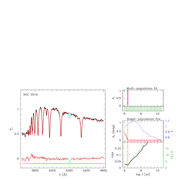
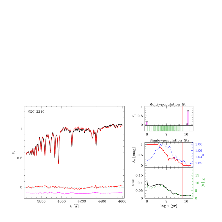
Fig. 1 shows the fit to NGC 2010 obtained with $Z$ fixed at $Z_{\odot}$. Insignificantly better ($\delta_{\chi^{2}}=0.01$) fits are obtained with the $1.5Z_{\odot}$ models. The left panel shows the observed, model, and residual spectra. The best match is obtained for $\log t=8.20$, $A_{V}=0.00$ and $x=1.03$. The middle right panel shows the runs of $A_{V}$ and $x$ as a function of $t$, while the bottom one shows the two indicators of fit quality discussed at the end of Section 4.3. The largest differences between $O_{\lambda}$ and $M_{\lambda}$ are found in the continuum between higher order Balmer lines and at the bottom of the CaII K line, but these are relatively small deviations. Overall, the spectral fit is very good both in the continuum and absorption lines.

Fig. 2 shows the results for NGC 2210 and $\log Z/Z_{\odot}=-1.7$. This is the $Z$ which produces the smallest $\chi^{2}$ among all 6 $Z$’s in the V00s models. Since $\log Z/Z_{\odot}=-1.7$ is also the smallest one in the grid, it is possible that models with even lower $Z$ would provide better fits. In this case differences between $O_{\lambda}$ and $M_{\lambda}$ concentrate around 4200 Å. The best fit is achieved for $\log t=9.80$ and $A_{V}=0.10$. Fits for younger ages require a larger extinction to compensate for the bluer predicted colors, but even then the quality of the fit deteriorates quickly as one moves away from the best $t$. Notice also that $A_{V}$ saturates at the imposed limits as one moves away from the best model.

5.2 The meaning of multi component fits

Accepting that SCs are single population systems, multi-SSP fits are in principle not of direct interest. Still, even if only out of curiosity, lets have a look at them.

The top right panel in Fig. 1 shows how the light at $\lambda_{0}$ is spread among SSPs of different ages in the multi-SSP starlight fit of NGC 2010. In this particular example, the multi-SSP fit is identical to the single-SSP one. In other words, given total freedom to mix 46 different base elements, starlight preferred to use only one. In the $Z=1.5Z_{\odot}$ fits (not shown), the multi-SSP fit splits into two similar parts, corresponding to populations within 0.1 dex of the best-fit single SSP age. The fit is thus well focused, such that multi and single SSP fits are almost identical.

The situation is very different in NGC 2210 (Fig. 2). The multi-SSP fit in this case shows two dominant components with ages over 2 dex apart: One with $\log t=10.10$, responsible for about 80% of the light, and other at the youngest age $\log t=8.00$, accounting for the rest. Unlike in Fig. 1, the difference between the multi and single-SSP spectra (shown in the bottom of the left panel) is now noticeable. Accordingly, the multi-SSP fit yields a $\chi^{2}$ which is 27% better than the single-SSP one (a difference which is of only 5% for NGC 2010).

A plausible interpretation of this “old plus a bit of young” population mixture, which happens in at least two other clusters in our sample, is that the SSP models lack old blue stars. This same problem was identified by K08 in a different sample. They found that clusters with a blue horizontal branch (HB) are better fitted adding a set of stars in the $T_{\rm eff}=6000$ to 20000 K range to a pure SSP. They also find that this ad hoc, but physically reasonable, recipe produces ages in better agreement with those derived from CMD studies. We will return to this issue in Section 7. For the moment, we note that the example of NGC 2210 fully corroborates this interpretation: The fiducial age adopted by LR03 is $\log t=10.1$, identical to that of the oldest population in our multi-SSP fits, but 0.3 dex older than the one obtained with a single-SSP fit ($\log t=9.80$).

These results show that multi-SSP fits provide an useful empirical measure of the adequacy of single-SSP fits. Six quantities are used to report results of the multi-SSP fits: The mean ($\overline{\log t}_{m}$) and standard deviation ($\sigma_{m}$) of $\log t$ (computed directly from the population vector $\vec{x}$ using equations 2 and 4 of Cid Fernandes et al. 2005), the age of the dominant population ($\log T_{m}$) and its corresponding percentage light fraction ($f_{m}$), plus the mean relative residual ($\overline{\Delta}_{m}$), and the difference in $\chi^{2}$ between the multi and single SSP fits ($\delta_{m}$), defined as in equation (6). These quantities are tabulated in Table 1, along with other results. For NGC 2010 (Fig. 1), for instance, we find $\overline{\log t}_{m}=8.12$, $\sigma_{m}=0.13$, and $\delta_{m}=5\%$, confirming a focused single SSP solution. On the other hand, for NGC 2210 (Fig. 2), $\overline{\log t}_{m}=9.74$, $\log T_{m}=10.10$, $\sigma_{m}=0.79$, and $\delta_{m}=27\%$, signalling the spread in ages discussed above. Section 7 elaborates on how these numbers can be used to identify suspicious fits.

5.3 Fits with different metallicities

Figure 3: Results of spectral fits of NGC 2010 with 6 different metallicities. Left: Run of best-fit $A_{V}$ (bottom), rms (middle) and $\delta_{\chi^{2}}$ (top) with age. Different lines correspond to different $Z$’s: magenta, blue, green, orange, brown and red correspond to $\log Z/Z_{\odot}=-1.7$, -1.3, -0.7, -0.4, 0, and +0.2, respectively. Circles mark the best-fit model for each $Z$. Right: Best fit SSP spectra for all 6 different $Z$’s. The observed model is in black and the model and residual spectra are plotted according to the color-scheme above. Note: The $O_{\lambda}-M_{\lambda}$ residual spectra are multiplied by 3 for clarity. Dashed horizontal lines at $y=-0.1$, 0 and $+0.1$ are drawn to facilitate comparisons. The best fit model ($\log Z/Z_{\odot}=+0.2$ in this case) is marked by a thicker window frame.

Figure 4: As Fig. 3 but for NGC 2210.

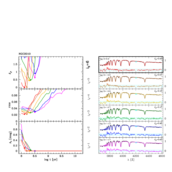
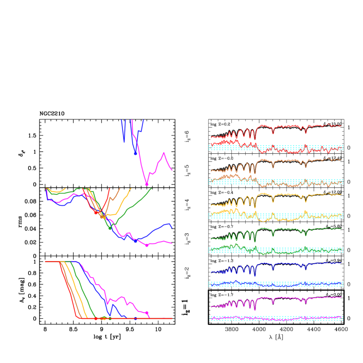
The example fits in Figs. 1 and 2 have fixed $Z$. In Figs. 3 and 4 we show how things change for different $Z$’s. The bottom-left panels show the best-fit $A_{V}$ as a function of age for all 6 metallicities. The middle panel show the rms of the single-SSP spectral fits, while the top panel shows $\delta_{\chi^{2}}$. Curves are color-coded according to $Z$, and a circle marks the location of the best model for the corresponding $Z$. Panels in the right show the best spectral fit achieved for each of the 6 metallicities. Residual spectra shown in these panels were multiplied by 3 for clarity.

Fig. 3 shows results for NGC 2010. Among all $6\times 46=276$ SSPs, the one with $\log Z/Z_{\odot}=+0.2$ and $\log t=8.11$ is the one which produces the best fit. Accordingly, this model has $\delta_{\chi^{2}}=0$. As already noted, the next best $Z$ is solar, for which $\delta_{\chi^{2}}=0.01$, i.e., its $\chi^{2}$ is just 1% worse than the best one! Visual inspection of the corresponding spectra confirms that these two solutions are indeed indistinguishable. Other metallicities produce visibly worse fits, suggesting that $Z$ is relatively well constrained to $\geq Z_{\odot}$ for this SC.

We note in passing that neither the rms (middle left panel) nor $\overline{\Delta}$ (not plotted) provide a strong numerical discrimination of different models. As can be seen in Fig. 3, the best models for different $Z$’s all yield numerically similar values for these figures of merit, even when the fits are visibly worse. Even if formally equivalent, the $\delta_{\chi^{2}}$ index is much more useful in this sense.

Results for NGC 2210 are shown in Fig. 3. In this case, there is a well defined metallicity: $\log Z/Z_{\odot}=-1.7$. The next best model ($\log Z/Z_{\odot}=-1.3$) has a nearly twice as bad $\chi^{2}$ ($\delta_{\chi^{2}}=0.94$). Fits for higher $Z$’s are so much worse that they fall off the top right panel.

5.4 Age-metallicity-extinction degeneracies

Figure 5: $\delta_{\chi^{2}}$ contours in the age-metallicity-extinction space for NGC 2010. The magenta line correspond to $\delta_{\chi^{2}}=1$ and the gray shaded area marks the $\delta_{\chi^{2}}\leq 0.5$ region. Blue, green and red correspond to 3, 2 and 1 sigma confidence regions, respectively. Best-fit values are marked with dotted lines. In the top panels a dashed line connects the best models for different $Z$’s.

Figure 6: As Fig. 5 but for NGC 2210.

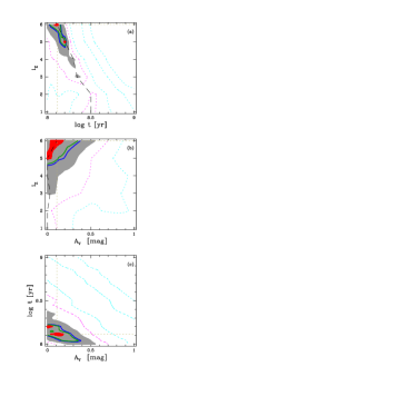
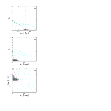
The plots above already show known couplings between parameters. The best way to visualize such covariances is through bidimensional $\Delta\chi^{2}$ maps.

Fig. 5 shows maps of $\delta_{\chi^{2}}$ in the three possible projections of the $t$-$Z$-$A_{V}$ space for NGC 2010. Notice that the $Z$ scale is not in physical units. Instead, we prefer to represent each of the 6 $Z$’s by a $i_{Z}=1$ to 6 metallicity index, a cosmetic choice which serves to emphasize the coarseness of the $Z$-grid. Dotted contours are for $\delta_{\chi^{2}}\geq 1$, the inner one ($\delta_{\chi^{2}}=1$) being drawn in magenta. The gray-shaded area maps the $\delta_{\chi^{2}}\leq 0.5$ zone, while the inner 3 contours mark the formal 3, 2 and 1 sigma ranges for our choice of $N_{dof}$ (see equation 7).

The well known trade-off between age and metallicity is evident in Fig. 5a. Notice also that solar and over-solar models are equally good, as noted before in Fig. 3, where best fit spectra for each $Z$ were shown. These two $Z$’s fall within the 1 sigma confidence region. In the case of NGC 2210, the “age-metallicity degeneracy” is not so evident because the best-fit metallicity is at the border of the $Z$-grid (Fig. 6a).

As $t$ and $Z$ assume only the discrete values dictated by the set of models used, such $\Delta\chi^{2}(t,Z)$ maps can be constructed directly from the output of the starlight fits. However, starlight only computes the best $A_{V}$ (and $x$) for each $(t,Z)$ pair, so some extra coding is needed to produce maps involving $A_{V}$. We have thus written a complementary code which, for each $t$ and $Z$, forces fits using $A_{V}$ values in a fine grid from 0 to 1. These fits have a single free parameter, $x$, whose optimal value is computed analytically from $\partial\chi^{2}/\partial x=0$. The resulting tables of $\chi^{2}$ as a function of $t$, $Z$ and $A_{V}$ can then be projected to $\Delta\chi^{2}(t,A_{V})$ and $\Delta\chi^{2}(Z,A_{V})$ maps.

As colors redden with increasing age and metallicity, one expects negative covariances between $A_{V}$ and both $t$ and $Z$. Such an “age-extinction degeneracy” is indeed observed in Fig. 5c (NGC 2010). The effect is also present, but much weaker, in NGC 2210 (Fig. 6c) where the trend is only noticeable in the $\delta_{\chi^{2}}\geq 0.5$ contours.

For many clusters, contours in the $A_{V}$-$Z$ plane show the expected “metallicity-extinction degeneracy”, but in these two examples it is not so clear. A hint of the expected effect is present in NGC 2210 (Fig. 6b), visible mainly from the outer contours, since the best fit values of $Z$ and $A_{V}$ are at a corner of the grid. In NGC 2010, however, the trend is opposite to the expected one, with contours showing positive covariance (Fig. 5b). In this case, the blueing of the continuum due to the decrease in $t$ as $Z$ increases (Fig. 5a) is larger than the reddening caused by the change in $Z$, explaining why $A_{V}$ increases with $Z$. This example serves as a reminder that the quantitative effects of the combination of $t$-$Z$-$A_{V}$ “degeneracies” can be more subtle than those expected on simple qualitative grounds.

These maps show that the $A_{V}\leq 1$ prior has very little effect. This happens because the extinction in our SCs is genuinely small. For the same reason, the physical $A_{V}\geq 0$ limit has more effect in constraining $A_{V}$, as seen, for instance, in the contours in Fig. 5b.

Before closing, we note that, as said in Section 4.3, the statistical interpretation of these surfaces can be adapted to other choices for $N_{dof}$. For instance, the $\delta_{\chi^{2}}=0.5$ shaded areas in Figs. 5 and 6 would correspond to 3 sigma contours ($\Delta\chi^{2}=11.8$ for a 2D projection) for $N_{dof}=24$, equivalent to considering every 34 Å of a spectrum as an independent datum.

5.5 Results for all clusters

Figure 7: All spectral fits, sorted by best-fit age. Observed and best fit single SSP spectra are shown in black and red, respectively, with the corresponding residual shown in green. Labels to the right of each spectrum list the best values of $\log t$ and $\log Z/Z_{\odot}$. All spectra are normalized at $\lambda_{0}=4020$ Å, and shifted vertically by 1 ($=$ one tick mark) from one another.

	Single population fits				Multi population fits					Bayesian estimates
Cluster	$\log t$	$\log Z/Z_{\odot}$	$A_{V}$	$\overline{\Delta}$	$\delta_{m}$	$\overline{\log t}_{m}$	$\sigma_{m}$	$\overline{\Delta}_{m}$	$\log T_{m}$ (%)	$\log t$	$\log Z/Z_{\odot}$	$A_{V}$
(1)	(2)	(3)	(4)	(5)	(6)	(7)	(8)	(9)	(10)	(11)	(12)	(13)
M 0411	9.10	-0.68	0.48	2.3	0.05	9.10	0.35	2.2	8.95 ($43$)	9.13 $\pm$ 0.10	-0.68 $\pm$ 0.20	0.41 $\pm$ 0.11
M 0416	9.90	-1.28	0.22	1.4	0.00	9.89	0.06	1.4	9.90 ($98$)	9.90 $\pm$ 0.01	-1.28 $\pm$ 0.00	0.22 $\pm$ 0.02
M 0419	9.10	-0.68	0.46	1.6	0.10	9.12	0.11	1.5	9.20 ($41$)	9.10 $\pm$ 0.00	-0.67 $\pm$ 0.06	0.46 $\pm$ 0.05
NGC 1651	9.35	-0.68	0.00	4.0	0.06	9.37	0.29	3.9	9.05 ($44$)	9.58 $\pm$ 0.19	-1.10 $\pm$ 0.34	0.36 $\pm$ 0.19
NGC 1754	9.80	-1.28	0.00	1.9	0.13	9.74	0.28	1.8	9.90 ($76$)	9.81 $\pm$ 0.03	-1.28 $\pm$ 0.04	0.02 $\pm$ 0.02
NGC 1783	9.25	-0.68	0.24	1.6	0.03	9.22	0.27	1.6	9.05 ($53$)	9.25 $\pm$ 0.06	-0.69 $\pm$ 0.13	0.26 $\pm$ 0.10
NGC 1795	9.70	-1.28	0.39	5.2	0.02	9.66	0.35	5.1	9.90 ($67$)	9.66 $\pm$ 0.16	-1.21 $\pm$ 0.25	0.38 $\pm$ 0.17
NGC 1806	9.25	-0.68	0.37	1.7	0.12	9.25	0.19	1.6	9.15 ($46$)	9.26 $\pm$ 0.02	-0.67 $\pm$ 0.03	0.34 $\pm$ 0.08
NGC 1818	8.00	-1.68	0.00	3.9	0.00	8.02	0.20	3.9	8.00 ($99$)	8.00 $\pm$ 0.00	-1.68 $\pm$ 0.00	0.02 $\pm$ 0.02
NGC 1831	8.75	-0.38	0.00	1.7	0.16	8.72	0.16	1.6	8.75 ($94$)	8.73 $\pm$ 0.03	-0.40 $\pm$ 0.08	0.03 $\pm$ 0.04
NGC 1846	9.25	-0.68	0.21	2.8	0.00	9.24	0.15	2.8	9.25 ($94$)	9.23 $\pm$ 0.07	-0.70 $\pm$ 0.13	0.27 $\pm$ 0.12
NGC 1866	8.04	0.20	0.55	1.9	0.04	8.08	0.12	1.9	8.00 ($70$)	8.05 $\pm$ 0.03	0.19 $\pm$ 0.07	0.53 $\pm$ 0.07
NGC 1978	9.40	-0.68	0.09	1.7	0.12	9.42	0.41	1.6	9.60 ($82$)	9.42 $\pm$ 0.11	-0.69 $\pm$ 0.10	0.11 $\pm$ 0.09
NGC 2010	8.11	0.20	0.11	2.0	0.05	8.12	0.13	2.0	8.00 ($54$)	8.14 $\pm$ 0.04	0.14 $\pm$ 0.09	0.09 $\pm$ 0.07
NGC 2121	9.90	-1.28	0.71	4.5	0.00	10.05	0.17	4.5	9.90 ($56$)	9.99 $\pm$ 0.19	-1.23 $\pm$ 0.17	0.55 $\pm$ 0.19
NGC 2133	8.26	0.20	0.31	2.1	0.09	8.32	0.15	2.0	8.26 ($77$)	8.27 $\pm$ 0.03	0.11 $\pm$ 0.10	0.33 $\pm$ 0.09
NGC 2134	8.45	-0.38	0.03	1.6	0.00	8.45	0.00	1.6	8.45 ($100$)	8.41 $\pm$ 0.08	-0.29 $\pm$ 0.19	0.09 $\pm$ 0.10
NGC 2136	8.04	-0.38	0.54	2.1	0.05	8.07	0.16	2.0	8.00 ($84$)	8.12 $\pm$ 0.11	-0.47 $\pm$ 0.19	0.40 $\pm$ 0.19
NGC 2203	9.35	-0.68	0.24	2.8	0.08	9.42	0.63	2.6	8.95 ($27$)	9.35 $\pm$ 0.05	-0.69 $\pm$ 0.09	0.25 $\pm$ 0.10
NGC 2210	9.80	-1.68	0.10	1.5	0.27	9.74	0.79	1.3	10.10 ($79$)	9.80 $\pm$ 0.00	-1.68 $\pm$ 0.00	0.10 $\pm$ 0.03
NGC 2213	9.30	-0.68	0.13	2.1	0.02	9.32	0.32	2.1	9.60 ($37$)	9.30 $\pm$ 0.00	-0.68 $\pm$ 0.01	0.13 $\pm$ 0.05
NGC 2214	8.04	-0.38	0.00	1.7	0.00	8.04	0.01	1.7	8.04 ($97$)	8.04 $\pm$ 0.01	-0.38 $\pm$ 0.01	0.02 $\pm$ 0.02
NGC 2249	8.85	-0.68	0.12	1.8	0.05	8.82	0.15	1.7	8.85 ($72$)	8.84 $\pm$ 0.02	-0.67 $\pm$ 0.04	0.15 $\pm$ 0.06
47 Tuc	10.00	-0.38	0.00	2.8	0.01	9.98	0.06	2.7	10.00 ($89$)	9.98 $\pm$ 0.05	-0.37 $\pm$ 0.04	0.02 $\pm$ 0.02
M 0015	9.80	-1.68	0.00	1.9	0.44	9.64	0.87	1.6	10.10 ($78$)	9.80 $\pm$ 0.00	-1.68 $\pm$ 0.00	0.02 $\pm$ 0.02
M 0079	9.80	-1.68	0.00	1.8	0.97	9.91	0.61	1.3	10.10 ($91$)	9.84 $\pm$ 0.11	-1.68 $\pm$ 0.00	0.01 $\pm$ 0.01
NGC 1851	10.20	-1.28	0.12	1.7	0.02	10.14	0.12	1.7	10.20 ($79$)	10.17 $\pm$ 0.04	-1.28 $\pm$ 0.00	0.11 $\pm$ 0.04

Table 1: Results for all clusters. Columns 2–5 correspond to the best single SSP fits; columns 6–10 list results of the multi-SSP fits (with $Z$ fixed and equal to that given in column 3); columns 11-13 list the Bayesian estimates of $t$, $Z$ and $A_{V}$.

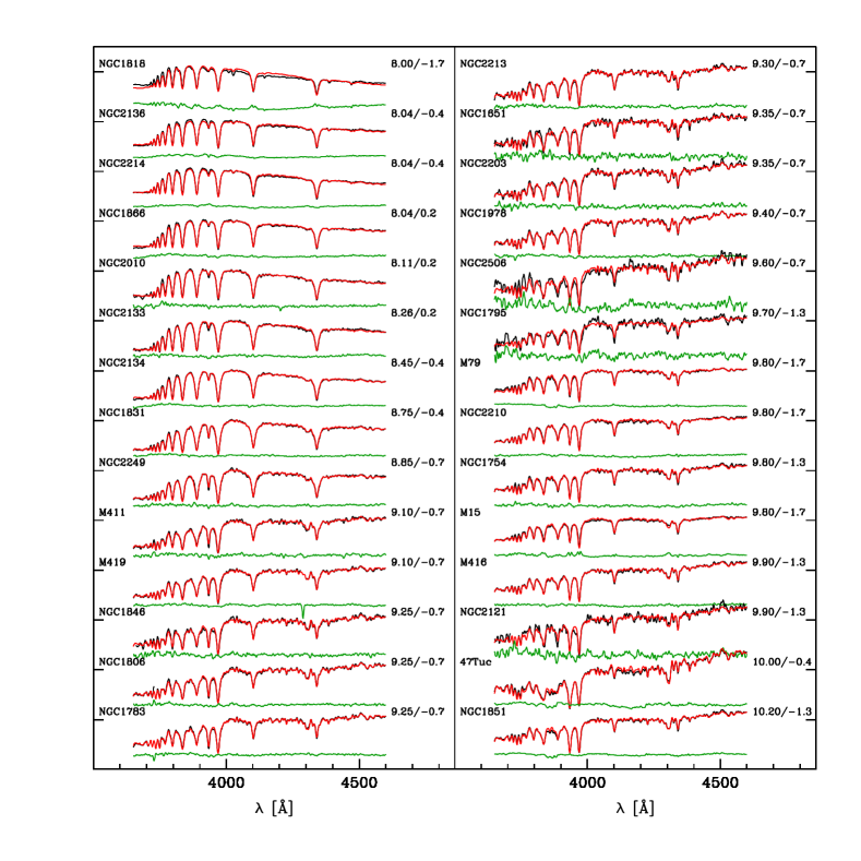
Columns 2–5 of Table 1 lists the best $t$, $Z$ and $A_{V}$ obtained for all 27 SCs in our sample. The corresponding value of $\overline{\Delta}$ is listed in column 6. Fig. 7 shows the corresponding spectral fits, sorted by the best-fit age. The first cluster shown, NGC 1818, is actually younger than 100 Myr, the smallest age available in the V00s models, and the fact that the best-fit is found for the lowest available $Z$ is an artificial consequence of this limitation. Our results for this SC should thus be ignored. The next three SCs (NGC 2136, NGC 2214, and NGC 1866) are also close to this limit, and results for them should be regarded with care, even though the fits are visibly better than in the case of NGC 1818.

6 Bayesian estimates of star cluster properties

The fits and $\Delta\chi^{2}$ maps presented above give an idea of the kind of precision in SC parameters achievable with spectral fits. So far, however, our assessment of the uncertainties was mostly qualitative. This section presents a simple Bayesian formalism adapted to the problem of SC parameter estimation. Revised estimates of $t$, $Z$ and $A_{V}$ are presented, along with their respective uncertainties.

6.1 Formalism

For a data set $D$ and a model with parameters $\vec{p}$, the posterior probability of $\vec{p}$ is given by Bayes theorem: $P(\vec{p}|D)=P(\vec{p})P(D|\vec{p})/P(D)$. For a $P(\vec{p})=$ constant prior and gaussian errors, $P(\vec{p}|D)\propto\exp[-\frac{1}{2}\chi^{2}(\vec{p})]$, from which estimates of any of the individual parameters in $\vec{p}$ can be obtained through marginalization.

Lets momentarily denote $t\equiv\log t$, $Z\equiv\log Z/Z_{\odot}$, and $A\equiv A_{V}$. Hence, $\vec{p}$ corresponds to $(t,Z,A,x)$, while the data $D$ correspond to an observed spectrum ($O_{\lambda}$) and its errors ($\epsilon_{\lambda}$). The posterior probability distribution function (PDF) of, say, the (log) age is then given by

$$P(t|D)=\int\int\int P(t,Z,A,x|D)\,dZ\,dA\,dx$$ (8)

and similarly for $Z$, $A$, and $x$.

Computing such multi-dimensional integrals is usually a cumbersome task, but with 4 dimensions the problem is still manageable and a simple discretization approach suffices. To evaluate the PDF of the parameters, one thus needs grids in $t$, $Z$, $A$ and $x$. Grids in $t$ and $Z$ are naturally available from the SSP models, while grids in $A$ were already computed to produce the $\Delta\chi^{2}(t,A_{V})$ and $\Delta\chi^{2}(Z,A_{V})$ maps shown above. The missing $x$-grid is the easiest to compute, as the effects upon $\chi^{2}$ of a change in $x$ with respect to the optimal value can be computed analytically. In this computation we restrict $x$ to the 0.8–1.2 range, a very generous prior, which, however, was not formally imposed in the single-population starlight fits presented in Section 5.

The $\Delta Z_{j}$ steps were computed as $[Z_{j+1}-Z_{j-1}]/2$ for intermediate $Z_{j}$’s, while the edge bins ($j=1$ and $N_{Z}$) were taken to be symmetric. The same scheme was followed for the other parameters, for which the sampling is much finer.

6.2 Results

Figure 8: Probability distribution functions for $t$, $Z$ and $A_{V}$ for NGC 2010. Solid lines correspond to PDFs with our fiducial choice for $N_{dof}$ (i.e., 61), whereas dotted (red) lines are for a 5 times smaller $N_{dof}$. A star marks the best fit value. One and two sigma error bars are also shown, centered on the mean values. In the top and middle panels, vertical lines mark ages and metallicities available in the set of evolutionary synthesis models used.

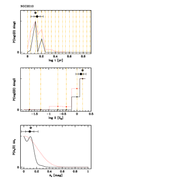
Results for NGC 2010 are shown in Fig. 8. In all panels, the solid curve corresponds to PDFs computed with our fiducial choice for $N_{dof}$ (see Section 4.3). The best fit value is marked by a star. The average value is plotted as a circle, and $\pm 1$ and $\pm 2$ sigma error bars (all computed directly from the PDF) are also drawn. The correspondance with the contour plots in Fig. 5 is evident. The two acceptable metallicities translate into the two peaks in $P(t)$. Two peaks are also seen in the PDF of $A_{V}$, but blended. Multi-modal PDFs and contour plots like these occur frequently, and are basically a by-product of the coarseness of the $Z$-grid (see Appendix A for results obtained with $Z$-interpolated grids). There are, however, exceptions. NGC 2210 is an example whose PDFs (Fig. 12) are unimodal and centered on the best fit values, as can be guessed from Fig. 6.

Just for illustrative purposes we also draw the PDF which would result from adopting a 5 times smaller $N_{dof}$. As expected, the PDFs become broader, but at least in this example, this extreme choice, which tantamounts to equalling a full spectral fit to fitting just $N_{\lambda}=16$ observables, the SC parameters are still well constrained.

The standard way of summarizing PDFs is to compute their average and standard deviation, as already done in Fig. 8. Results for all clusters are listed in the last 3 columns of Table 1. These are our official estimates for the SC properties and their uncertainties. Note, however, that the table contains several entries for which $\sigma(\log Z)$ is very small or even zero! This is obviously wrong physically and statistically, but is a direct mathematical consequence of the coarseness of the $Z$-grid (see Appendix A). In such cases, NGC 2210 being an example, the likelihood is so concentrated around one $Z$ that neighboring grid points contain essentially no “probability mass”. When this happens, it is prudent to adopt something like half the $\log Z$-grid separation as a measure of $\sigma(\log Z)$. (The mean half grid separation is 0.2 dex in metallicity and 0.025 dex in age.) Also, as already noted, results for clusters too close to the age and metallicity limits of the models should be read with caution.

Typical (sample mean) formal statistical uncertainties in $\log t$, $\log Z/Z_{\odot}$ and $A_{V}$ are 0.06 dex, 0.09 dex and 0.08 mag. No trend of uncertainty with mean SC properties was found. Notice that the typical uncertainty in $\log t$ is nearly identical to the 0.05 dex age spacing of the V00s models, so, besides a finer $Z$-grid, a finer sampling in age would also be desirable.

Simulations which test the ability of the spectral synthesis methodology used in this paper to recover SC parameters under different levels of noise are described in Appendix B. The overall conclusion of these simulations is that the method is robust. For $S/N>30$ (as most of the data used in this paper) one expects bayesian estimates within $<0.1$ dex in age, $<0.2$ dex in metallicity and $<0.1$ dex in $A_{V}$ of the correct values.

7 Summary and Discussion

We have presented a rigorous but straightforward methodology to fit SC spectra with predictions from modern, publicly available high resolution evolutionary synthesis models. The method is mostly based on the also publicly available (but never before used for SCs) spectral synthesis code starlight, from which one can derive best $t$ and $Z$ estimates, as well as likelihood maps in the $(t,Z)$ plane. Objective recipes to deal with the absence of errors and account for spectral resolution in the definition of the effective number of degrees of freedom were presented. A simple bayesian approach was followed to compute formal probability distribution functions for the parameters. The method was applied to 27 SCs from the work of Leonardi & Rose (2003), modelled with publicly available SSP models of Vazdekis et al. (2009) based on the MILES library, “Padova 2000” tracks and a Salpeter IMF.

The main goal of this paper was to setup and illustrate this methodology, paving the way for the comparative study presented in Paper II, where results obtained with different models are presented and compared to independent work. This comparison is essential to map systematic uncertainties, whereas in this paper only statistical uncertainties were addressed.

A first general result is that the spectral fits are very good, yielding residuals of the order of $\overline{\Delta}=2\%$, equivalent to a signal-to-noise ratio of 50. That, of course, does not guarantee that the inferred parameters are correct. Insofar as $A_{V}$ is concerned, our results are consistent with previous estimates, which indicate very low extinction for SCs in this sample (e.g., Bica & Alloin 1986). In Paper II we show that, taking CMD determinations of $t$ and $Z$ as a reference, spectral fitting does provide reliable results.

Regarding the estimation of SC properties, the coarseness of the available models in $Z$ introduces some undesirable complications, like probability islands in the parameter space, reflected as multimodal PDFs of age and extinction. In cases where one $Z$ is highly preferred, the lack of a finer grid leads to an underestimation of the statistical uncertainties in the SC parameters. Experiments with $Z$ interpolated spectra alleviate these problems to some extent, but the ultimate solution is to have a finer sampling in both $Z$ and $t$.

Figure 9: Multi-SSP age dispersion plotted in the $t$-$Z$ plane, where $\langle\log t\rangle$ and $\langle\log Z/Z_{\odot}\rangle$ given by our Bayesian estimates. The size of the circles scales with $\sigma_{m}$ (the age dispersion in the multi-SSP fits), which ranges from 0 to 0.9 dex. Red circles correspond to cases where multi-SSP fits are much better than single SSP ones ($\delta_{m}>20\%$), while green is used when $\delta_{m}<10\%$ and blue correspond to cases in between. Large $\sigma_{m}$, like those seen for leftmost sources (M15, M79 and NGC 2010), is indicative of a component not adequately represented in the models, like blue HB stars. NGC 1818 is not plotted because it is younger than the lower age in the V00s models.

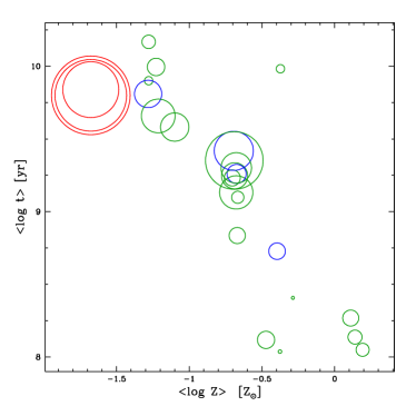
A curious effect found in some of the multi-SSP fits was a split into a light dominating old population ($\sim 80\%$) and weaker ($\sim 20\%$) but significant population of much younger age (often the lowest age in the grid), as if the SSP model spectra lacked old blue stars. In principle, these multi-component starlight fits should not be relevant for SCs, but we find that they are able to capture symptoms of inadequate single SSP fits in a quantitative manner. Clusters with suspicious combinations of different ages may be identified by large values of $\sigma_{m}$ (ie., large dispersions in $\log t$). Four clusters have $\sigma_{m}>0.6$: M15, M79, NGC 2203, and NGC 2210 (Figs. 2 and 6). M15 and M79 are very similar to NGC 2210. In fact, they all have identical best fit $t$ and $Z$, as well as the same $\log T_{m}$, similar $f_{m}$, and $\delta_{m}$ values which indicate that the multi-SSP fit is substantially better than a single SSP fit ($\delta_{m}=44\%$ for M15, $97\%$ for M79, and $27\%$ for NGC 2210). NGC 2203, on the other hand, is only similar to NGC 2210 in terms of $\sigma_{m}$, and its multi-SSP fit is not substantially better than single SSP one ($\delta_{m}=8\%$). Thus, the “old plus young” anomaly is only convincingly detected in M15, M79 and NGC 2210.

Following K08, we suggest this result is due to incomplete modelling of the horizontal branch (HB). CMD work on M15 (Battistini et al. 1985; Buonanno et al. 1983), M79 (Kravtsov et al. 1997) and NGC2210 (Brocato et al. 1996) have shown that all these clusters have blue HBs, which supports our interpretation of the spectral synthesis results. Alternatively, blue stragglers would have a similar effect. Combinations of UV and optical photometry detect the presence of these stars in M15 (Guhathakurta et al. 1993; Ferraro & Paresce 1993) and M79 (Lanzoni et al. 2007). The situation is less clear in NGC 2210. Based on the similarity of NGC 2210 HST CMD to NGC 2257, Johnson et al. (1999) suggest that the cluster have both a blue HB and blue stragglers, while Brocato et al (1996) have argued (on the basis of a ground based CMD) that the stars in the blue straggler region are likely field contaminants in NGC 2210.

In broad terms, one expects bluer HB at lower $Z$ (Harris 1996; Greggio & Renzini 1990), and hence the age-spread noticed in the multi-SSP fits should increase for decreasing $Z$. Fig. 9 presents tentative evidence of this relation. SCs with large $\sigma_{m}$ and $\delta_{m}$ tend to be those with smallest $Z$. Because $Z$ and $t$ are strongly anti-correlated in this sample, the highest $\sigma_{m}$ clusters are also among the oldest ones. Given that $Z$ is not the single factor determining HB morphology, not to mention other possibilities (like blue stragglers and stochastic effects) and uncertainties involved, we shall not elaborate further on this issue.

Figure 10: Extension of statistically indistinguishable fits to the 3650–4600 Å data to the red limit of the models for 4 SCs. For each cluster, the red and green lines are fits with different metallicities ($\log Z/Z_{\odot}=-1.3$ and $-0.7$ for NGC 1651 and NGC 1795, and $\log Z/Z_{\odot}=0$ and $+0.2$ for NGC 2133 and NGC 2010). The observed spectra are plotted in black.

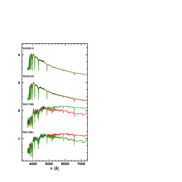
Moving away from caveats in the stellar population issues, we must acknowledge at least one limitation of our results: Wavelength coverage. The spectra used here cover a relatively small region in the blue–near-UV. Not only it misses some strong $t$ and $Z$ sensitive absorption features, like H$\beta$ and the MgI lines, but the lack of a wider baseline prevents a firmer handle on $A_{V}$. No doubt a wider coverage would help better constrain SC properties, but how much? Could more data help, for instance, lifting the ambiguities in $Z$ found for several SCs?

A qualitative answer to this question is given in Fig. 10, where, for each of four SCs, we plot the two best SSP fits with different $Z$, extending it from the 3650–4600 Å range covered by the data to the red limit of the V00s models. For the two clusters at the bottom of the plot, NGC 1651 and NGC 1795, for which $\log Z/Z_{\odot}=-1.3$ and $-0.7$ provide statistically indistinguishable fits, the extrapolated model spectra differ a lot both in continuum shape and in the depth of absorption features to the red of 4600 Å. In these cases, data in the red would clearly help distinguishing the fits. For NGC 2010 and NGC 2133, on the other hand, spectra in the red would not be as useful, as the extrapolated models are essentially indistinguishable. A wider baseline would be needed to pin down the best solution in these younger systems.

Appendix A Interpolations in metallicity

In the absence of a fine $Z$-grid, one may resort to interpolations. Because of stellar evolution effects, interpolating in $Z$ at fixed $t$ is not strictly valid, but one expects it to work at least approximately. This appendix describes results of experiments with $Z$-interpolated models. The original $N_{Z}=6$ grid was interpolated to $N_{Z}=39$ with $\log Z/Z_{\odot}$ between $-1.7$ and $+0.2$ in 0.05 dex steps. The spectral interpolations were carried out in log-log space, with $\log F_{\lambda}(t;Z)=a_{\lambda}(t)\log Z/Z_{\odot}+b_{\lambda}(t)$.

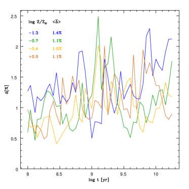
To test how well $Z$-interpolation works we have compared the original $\log Z/Z_{\odot}=-1.3$, $-0.7$, $-0.4$ and $0.0$ spectra with those obtained through interpolation of models with adjacent $Z$-values (for instance, using the $-1.3$ and $-0.4$ models to interpolate to $-0.7$). The results are shown in Fig. 11, where we plot the mean percentage spectral deviation $\overline{\Delta}$ against $t$ for each of these four intermediate $Z$’s. The residuals are computed after re-normalizing the spectra at 4020 Å, eliminating differences in the absolute flux scale. The plot shows that interpolation leads to typical errors of 1% in terms of spectral residuals, but that in many cases $\overline{\Delta}$ approaches or even exceeds 2%. These residuals are of the same order of the $\overline{\Delta}$ values obtained in fits of actual SCs (Table 1)! Naturally, in these tests the interpolations are based on models farther apart in $Z$ than when using the full grid. Nevertheless, we take these results as a signal that an interpolated grid may not lead to as much improvement as one would hope to achieve.

Figure 11: Mean percentage spectral residual ($\overline{\Delta}$) as a function of age for $Z$-interpolated models as compared to the original ones for $\log Z/Z_{\odot}=-1.3$, $-0.7$, $-0.4$ and $0.0$. Average values of $\overline{\Delta}$ for all ages are listed in the inset table. The message from this plot is that interpolating SSP spectra in $Z$ introduces errors which are of the same order as the spectral residuals obtained in fits of actual SC data.

Figure 12: Comparison of the $t$, $Z$ and $A_{V}$ PDFs obtained with the original (dotted red lines) and $Z$-interpolated grids (solid black), for three SCs in our sample. As in Fig. 8, a star marks the best-fit value, and the filled circle marks bayesian estimate. Error bars are also shown.

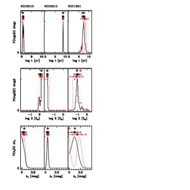
We now check how a finer $Z$-grid changes our parameter estimates. Fig. 12 shows the marginalized PDFs of $t$, $Z$ and $A_{V}$ for NGC 2010, NGC 2210 and NGC 1651. The plot compares the PDFs derived with the original $N_{Z}=6$ Z-grid (dotted red lines) with those derived with the $N_{Z}=39$ interpolated models (solid black). For NGC 2010 and NGC 2210 the $Z$-interpolated PDFs do not differ significantly from the original ones. The clearest changes are in the PDF($A_{V}$) for NGC 2010, which becomes smoother (single-peaked), and in the PDF($Z$) for NGC 2210, which rises steeply towards $\log Z/Z_{\odot}=-1.7$ (confirming that the lowest $Z$ models are indeed the ones which better fit the data for this SC). More significant changes occur in the case of NGC 1651. With the $Z$-interpolated models, PDF($t$) has a pronounced peak in between the two peaks obtained with the original grid. Similarly, the PDF($Z$) now peaks in between the two original $Z$ values with highest probability. The more dramatic change is in PDF($A_{V}$), whose original two peaks merge into a single one at an intermediate value of $A_{V}$. For all three parameters the $Z$-interpolated models produce more focused PDFs, and thus smaller formal uncertainties (see error bars in the NGC 1651 panels of Fig. 12). Notwithstanding these apparently large differences, the bayesian estimates of $t$, $Z$ and $A_{V}$ derived with the coarser original $Z$-grid are consistent with those derived with the better sampled interpolated $Z$-grid. They are also more conservative, in the sense of having larger error bars.

Considering the sample as a whole, we detect no bias between parameters estimated with the original and $Z$-interpolated grids. The rms difference in the bayesian estimates of $\log t$ and $\log Z/Z_{\odot}$ are just 0.08 and 0.12 dex respectively, while for $A_{V}$ the rms difference is 0.08 mag. $Z$-interpolated grids produce better spectral fits, but only marginally so. In terms of the $\overline{\Delta}$ figure of merit, the $Z$-interpolated fits yield a sample-average value of $\overline{\Delta}=2.39\%$, compared to 2.44% obtained with the original grid.

Regarding formal (PDF-based) parameter uncertainties, our experiments show that when an uncertainty derived with the original grid is “large” ($\ga 0.05$ dex in $\log t$, $\ga 0.15$ dex in $\log Z/Z_{\odot}$, and $\ga 0.1$ mag in $A_{V}$), it tends to be smaller with the $Z$-interpolated grid, and vice versa. This behavior is consistent with qualitative expectations. In cases where a PDF is unresolved due to a coarse grid, leading to a formal error of zero, interpolation resolves the PDF, producing a measurable second moment (standard deviation $>0$). For instance, for NGC 2210 we find $\sigma(\log Z)=0$ with the original grid (all probability is in the first $Z$-bin), and 0.02 dex with the interpolated one. Conversely, when, say, the PDF of $Z$ is spread over two or more adjacent original $Z$-bins, a finer grid may produce a more focused (narrower) PDF, as in the case of NGC 1651. In any case, these are relatively small differences, such that the sample-average uncertainties derived with both methods are virtually indistinguishable.

All in all, we see no major gain in resorting to $Z$-interpolated models. Further considering the uncertainties introduced by such interpolations (Fig. 11), we think it is safer to wait for properly computed, finer $Z$-grids to be released by than to interpolate in $Z$.

Appendix B Effects of data quality

The starlight code, used throughout this paper, has been extensively used and tested in the context of mixed stellar populations (galaxies), but this is the first time it is used to fit SCs. This appendix presents simulations designed to evaluate the reliability of SC properties derived with this code under different levels of noise.

To test the effects of data quality, we have performed simulations in which white gaussian noise is added to a model SSP spectrum of known $t$, $Z$ and $A_{V}$. These perturbed spectra are processed exactly as the observed ones, and input and output parameters are then compared. The input models were built using the V00s SSPs which best fit the 27 actual SCs in our sample, whose properties are listed in columns 2–4 of Table 1. Their corresponding spectra were taken directly from starlight’s output, and thus mimic the actual data in terms of wavelength coverage and resolution. Five realizations of a noise spectrum ($n_{\lambda}$) were generated, and five others were derived from these by inverting the sign of $n_{\lambda}$. These 10 perturbation spectra were scaled to emulate $S/N$ ratios between 10 and 95.

Figure 13: Illustration of the effects of noise upon derived SC properties for simulations based on the $t$, $Z$ and $A_{V}$ values obtained for NGC 1651 (top panels), NGC 1795 (middle) and NGC 2010 (bottom). The 1st and 2nd columns of plots show results of the analysis of two individual perturbed spectra. Error bars and the shaded area show the PDF based $\log t\pm\sigma(\log t)$, and similarly for $\log Z$ and $A_{V}$, while the (green) star marks the best-fit value. The last column shows the statistics of the simulations. In this case the shaded area shows the mean and $\pm$ one sigma range of the PDF based values of $\overline{\log t}$, $\overline{\log Z}$ and $\overline{A_{V}}$. The points with error bars (in red) show the mean and standard deviation of the best-fit values among 10 realizations of the noise for each $S/N$.

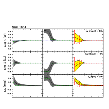
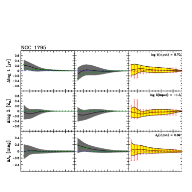
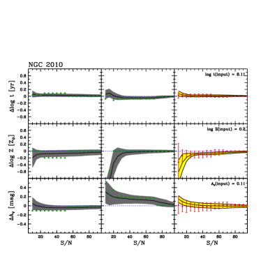
Fig. 13 illustrates the results for three test SCs, with parameters based on those found for NGC 1651, NGC 1795 and NGC 2010. All panels show output minus input parameters against the $S/N$. The left and middle columns show, for each $S/N$, the results of an analysis based on an individual spectrum. The examples picked for these panels differ only in the sign of the perturbation, such that if in the left column the spectrum feed into starlight is $F_{\lambda}+n_{\lambda}$, in the middle one the analysis is carried out with $F_{\lambda}-n_{\lambda}$. Also, $n_{\lambda}$ has the same shape for all $S/N$ values, such that the only thing that changes along the $x$-axis is the amplitude of the noise. This cosmetic choice is done only for presentation purposes, as it produces more illustrative plots than obtained picking perturbed spectra at random. Finally, the third column of plots shows statistical results considering all 10 spectra available at each $S/N$.

Consider first the left and middle panels. Stars show the difference between best fit and input values of $\log t$, $\log Z$ and $A_{V}$ as a function of $S/N$. The solid line shows the differences between the bayesian estimates and the input values, while the grey shaded areas show the corresponding $\pm$ one sigma formal (PDF-based) uncertainty. Besides the expected convergence as $S/N$ increases, these plots illustrate covariances between age, metallicity and extinction. When the $Z$-estimate does not change, underestimated $t$’s are compensated by overestimated $A_{V}$’s, and vice-versa, as in the left panels for NGC 1651 and in the left and middle panels for NGC 1795. In the middle panel for NGC 1651, one sees that both $t$ and $A_{V}$ are overestimated at low $S/N$ due to the fact that fits with the $\log Z/Z_{\odot}=-1.3$ grid point are preferred over the $\log Z/Z_{\odot}=-0.7$ original value. In this particular example, only for $S/N\geq 30$ the input parameters are well recovered. In the case of NGC 2010, the left panels show that solutions oscillate between $Z=1.5Z_{\odot}$ (the input value) and $Z_{\odot}$, and all SC parameters vary in concert. This metallicity confusion occurs for $S/N$ as large as 50, which is not surprising, given the high degree of spectral similarity between solar and over-solar V00s models in this age range (see Fig. 3). In the example examined in the middle panels, $Z$ comes out badly underestimated for $S/N\leq 15$. Above that $Z$ is well recovered, but minor differences in $A_{V}$ and $t$ can persist to $S/N$ as high as 70.

These examples illustrate what may happen in the analysis of individual spectra observed under different regimes of $S/N$. The general message spelt by these simulations is that, when dealing with one single object and using only the kind of observational data used in this paper, one should be careful about biases in parameter estimates obtained through spectral synthesis if $S/N\la 30$. Beyond this $S/N$, output minus input deviations are too small to worry about.

The right panels in Fig. 13 show the results of a statistical analysis of all perturbed spectra for each test-SC. The yellow shaded ranges marks the dispersion in the bayesian estimates of $\overline{\log t}$, $\overline{\log Z}$, and $\overline{A_{V}}$ among the 10 perturbed versions of a same spectrum. Similarly, the red error bars show the dispersion in the best fit estimates as a function of $S/N$. The sometimes large deviations observed in the left and middle panels average out in these statistical results. Biases in the estimates are still present at low $S/N$, but almost always within one sigma of output $=$ input. The most noticeable bias in the right panels of Fig. 13 occurs for $A_{V}$ in NGC 1651, and only for low $S/N$. Since $A_{V}<0$ was forbidden in the fits, and the input value of $A_{V}$ is exactly zero in this case, one can only err upwards, so this bias can be understood as an edge effect.

Fig. 14 summarizes the statistics of the noise-induced variations in bayesian parameter estimates for all 27 test SCs. The top panels, show the standard deviation (considering the 10 perturbations) of the $\overline{\log t}$ estimate against the input value of $\log t$ for three values of $S/N$: 10 (red open circles), 20 (green open squares) and 30 (blue filled triangles). Dotted lines mark the average $\sigma(\overline{\log t})$ for these 3 values of $S/N$. The plot shows that the typical uncertainties in $\overline{\log t}$ due to noise are of $<0.2$ dex for $S/N>10$. For SCs in the 9.0 to 9.5 $\log t$ range the uncertainty reaches 0.3 dex for $S/N=10$, which is acceptable considering such low quality data. The middle and bottom panels show the results for $\log Z/Z_{\odot}$ and $A_{V}$. For the metallicity, noise at a $S/N=10$ level introduces up to 0.5 dex uncertainty, but the overall average value is 0.3 dex. As for the ages, the uncertainty in $Z$ peaks at intermediate values. A plausible explanation for this is that in the middle of a ($t$ or $Z$) grid one can look to either side and find reasonably similar spectra, whereas closer to the edges there is not so much option, thus reducing the ranges in $t$ and $Z$ where statistically acceptable fits can be found. For $A_{V}$ we find up to 0.2 mag uncertainty, with a typical value of 0.1 mag.

Figure 14: Statistical uncertainties on $\overline{\log t}$ (top panel), $\overline{\log Z}$ (middle) and $\overline{A_{V}}$ (bottom) for simulations with $S/N=10$ (red open circles), 20 (green open squares) and 30 (blue solid triangles). Dotted horizontal lines mark the mean value over all 27 simulated clusters. Each point corresponds to results from 10 Monte Carlo realizations of the noise. The 27 points (for each $S/N$ level) correspond to test clusters whose parameters are identical to those in columns 2–4 of Table 1.

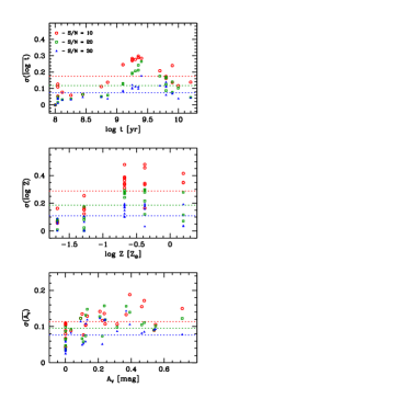
The overall conclusion of these experiments is that, for the kind of data used in this paper (medium resolution spectra in the blue range), $S/N\ga 30$ is required to accurate SC parameter estimates from spectral synthesis of an individual object. When large samples of objects are analyzed, one can trust statistical results obtained with lower quality data.

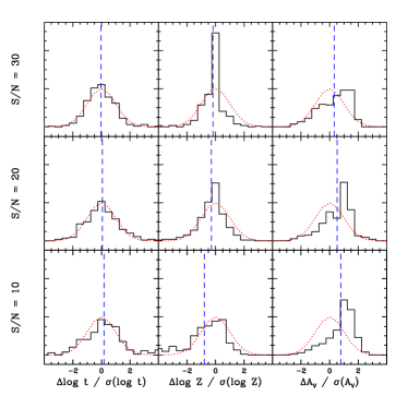
We emphasize that our conclusion that $S/N\ga 30$ is required to produce accurate parameter estimates is not equivalent to saying the method fails at lower $S/N$. Our simulations show that, as expected, output minus input differences in SC properties tend to increase as $S/N$ decreases, but so do the associated error bars. The reliability of a parameter estimation method is better measured not in terms of absolute differences, but in terms of differences in units of the associated uncertainty, e.g., $[\overline{\log t}-\log t(\rm input)]/\sigma(\log t)$. Evaluated in this way, spectral synthesis is capable of producing good results for any of the $S/N$ investigated. This is illustrated in Fig. 15, which shows histograms of output minus input parameters in units of the corresponding formal uncertainty. All 10 perturbed versions of all 27 SCs are included in these histograms. Bottom, middle and top panels show results for $S/N=10$, 20 and 30, respectively. Dotted lines draw gaussians of unit $\sigma$ and normalized to the same area. The histograms follow quite well the the gaussian expected in the ideal case, with the noticeable exception of $A_{V}$, which is systematically overestimated as a result of the already mentioned $A_{V}\geq 0$ edge effect. For $S/N=10$ this bias is close to 1 sigma, as can be seen by the location of the vertical dashed line, which marks the average value of $[\overline{A_{V}}-A_{V}(\rm input)]/\sigma({A_{V}})$. For $S/N=20$ this difference reduced to 0.5 sigma on average, while for better data the distribution of $[\overline{A_{V}}-A_{V}(\rm input)]/\sigma({A_{V}})$ becomes progressively less skewed. Another effect which can be noticed in this plot is that for high $S/N$ the distribution of $[\overline{\log Z}-\log Z(\rm input)]/\sigma(\log Z)$ becomes narrower than expected. This happens because as the noise decreases the PDF of $Z$ becomes increasingly focused and centered on the correct grid-value of $Z$, and hence $\overline{\log Z}=\log Z(\rm input)$.

Figure 15: Distribution of the difference between the output bayesian estimate and the input parameter in units of the formal uncertainty for $\log t$ (left), $\log Z$ middle, and $A_{V}$ (right). Vertical dashed lines mark the average value of the normalized difference. Dotted lines (in red) correspond to gaussians of unit standard deviation and normalized to the same area as the simulated data. The histograms include results for 270 runs, corresponding to 10 perturbations of the 27 test-SCs. Botttom, middle and top panels correspond to simulations with $S/N=10$, 20 and 30, respectively.

References

- Asari et al (2007) Asari N. V., Cid Fernandes R., Stasinska G., Torres-Papaqui J. P., Mateus A.; Sodré L., Schoenell W., Gomes J. M., 2007, MNRAS, 381, 263
- Barth et al. (2002) Barth A. J., Ho L. C., Sargent W. L. W., 2002, AJ, 124, 2607
- Battistini et al. (1985) Battistini, P., Bregoli, G., Fusi Pecci, F., Lolli, M., & Epps Bingham, E. A. 1985, A&AS, 61, 487
- Bica & Alloin (1986) Bica E., Alloin D., 1986, A&A, 162, 21
- Brocato et al. (1996) Brocato, E., Castellani, V., Ferraro, F. R., Piersimoni, A. M., & Testa, V. 1996, MNRAS, 282, 614
- Bruzual (2007) Bruzual G. 2007, in ”The Interplay Among Black Holes, Stars, and ISM in Galactic Nuclei”, eds. T. Storchi-Bergmann, L.C. Ho, and H.R. Schmitt, Cambridge: Cambridge University Press, 121-126
- Bruzual & Charlot (2003) Bruzual G., Charlot S., 2003, MNRAS, 344, 1000
- Buonanno et al. (1983) Buonanno, R., Buscema, G., Corsi, C. E., Iannicola, G., & Fusi Pecci, F. 1983, A&AS, 51, 83
- Cardelli et al (1989) Cardelli J. A., Clayton G. C., Mathis J. S., 1989, ApJ, 345, 245
- Cid Fernandes et al. (2005) Cid Fernandes R., Mateus A., Sodré L., Stasińska G., Gomes J. M., 2005, MNRAS, 358, 363
- Cid Fernandes (2007) Cid Fernandes R., on Stellar Populations as Building Blocks of Galaxies, Proceedings of IAU Symposium 241. Edited by A. Vazdekis and R. F. Peletier. Cambridge: Cambridge University Press, 2007, p. 461-469
- Cid Fernandes et al. (2009) Cid Fernandes, R., Schoenell W., Gomes J. M., Asari N. V., Schlickmann M., Mateus A., Stasińska G., Sodré L. Jr., Torres-Papaqui J. P., 2009, RMxAC, 35, 127
- Ferraro & Paresce (1993) Ferraro, F. R., & Paresce, F. 1993, in “Structure and Dynamics of Globular Clusters”, Editors, S.G. Djorgovski and G. Meylan; Astronomical Society of the Pacific, Vol. 50, P.299
- Garcia et al. (2005) Garcia-Rissmann A., Vega, L. R., Asari N. V., Cid Fernandes R., Schmitt H., González Delgado R. M., Storchi-Bergmann T., 2005, MNRAS, 359, 765
- Geisler et al. (2002) Geisler D. P., Grebel E. K., Minniti D., 2002, in ”Extragalactic star clusters”, the 207th symposium of the IAU , eds. Geisler, Douglas Paul.; Grebel, Eva K.;Minniti, Dante. 2002, Astronomical Society of the Pacific
- Girardi et al. (2000) Girardi L., Bressan A., Bertelli G., Chiosi C., 2000, A&A, 141, 371
- Girardi et al. (2002) Girardi L., Bertelli G., Bressan A., Chiosi C., Groenewegen M. A. T., Marigo P., Salasnich B., Weiss A., 2002, A&A, 391, 195
- González Delgado (2009) González Delgado R. M., 2009, ApSS, in press
- Gomes (2009) Gomes J. M., 2009, PhD Thesis, Universidade Federal de Santa Catarina
- Gordon et al. (2003) Gordon K. D., Clayton G. C., Misselt K. A., Landolt A. U., Wolff M. J., 2003, ApJ, 594, 279
- Greggio (1990) Greggio L., Renzini A., 1990, ApJ, 364, 35
- Guhathakurta et al. (1993) Guhathakurta, P., Yanny, B., Schneider, D. P., & Bahcall, J. N. in “ Blue Stragglers”. ASP Conference Series; Vol. 53; R.A. Saffer; Ed., p.60
- Harris (1996) Harris W., 1996, AJ, 112, 1487
- Johnson et al. (1999) Johnson, J. A., Bolte, M., Stetson, P. B., Hesser, J. E., & Somerville, R. S. 1999, ApJ, 527, 199
- Koleva et al (2008) Koleva M., Prugniel Ph., Ocvirk P., Le Borgne D., Soubiran, C., 2008, MNRAS, 385, 1998
- Koleva et al (2009) Koleva M., Prugniel P., De Rijcke S., 2009, Astron. Nachr. /AN 999, No. 88, 1
- Kravtsov et al. (1997) Kravtsov, V., Ipatov, A., Samus, N., Smirnov, O., Alcaino, G., Liller, W., & Alvarado, F. 1997, A&AS, 125, 1
- Lacon et al (2009) Lançon A., Fouesneau M., 2009, in ”Hot and Cool: Bridging Gaps in Massive Star Evolution”, ed. C. Leitherer, Ph. D. Bennett, P. W. Morris, J. Th. van Loon (San Francisco: ASP), in press, arXiv:0903.4557
- Lamers et al. (2004) Lamers H. J. G. L. M., Smith L. J., Nota A., 2004, The Formation and Evolution of Massive Young Star Clusters, 322,
- Lanzoni et al. (2007) Lanzoni, B., et al. 2007, ApJ, 663, 1040
- le Borgne et al. (2003) Le Borgne J.-F., et al., 2003, A&A, 402, 433
- le Borgne et al. (2004) Le Borgne D., Rocca-Volmerange B., Prugniel P., Lançon A., Fioc M., Soubiran C., 2004, A&A, 425, 881
- Leonardi & Rose (2003) Leonardi A. J., Rose J. A., 2003, ApJ, 126, 1811
- Perez el at (2009) Pérez E., de Grijs R., González Delgado R. M., 2009, in ’Young massive star clusters”, ApSS, in press
- Salpeter (1955) Salpeter E. E., 1955, ApJ, 121, 161
- Sánchez-Bláquez et al. (2006) Sánchez-Blázquez P., et al., 2006, MNRAS, 371, 703
- Schiavon et al. (2005) Schiavon R. P., Rose J. A., Courteau S., MacArthur L. A., 2005, ApJS, 160, 163
- Vazdekis (1999) Vazdekis A., 1999, ApJ, 513, 224
- (39) Vazdekis A., et al. 2009, MNRAS, submitted.
- Wolf et al. (2007) Wolf M. J., Drory N., Gebhardt K., Hill G. J., 2007, ApJ, 655, 179
- Zaritsky et al. (2004) Zaritsky, D., Harris, J., Thompson, I. B., & Grebel, E. K. 2004, AJ, 128, 1606