Elementary Energy Release Events in Flaring Loops: Effects of Chromospheric Evaporation on X-rays

Abstract

With the elementary energy release events introduced in a previous paper (Liu & Fletcher, 2009) we model the chromospheric evaporation in flaring loops. The thick-target hard X-ray (HXR) emission produced by electrons escaping from the acceleration region dominates the impulsive phase and the thin-target emission from the acceleration region dominates the low-energy thermal component in the gradual phase, as observed in early impulsive flares. Quantitative details depend on properties of the thermal background, which leads to variations in the correlation between HXR flux and spectral index. For lower temperature and/or higher density of the background electrons, the HXRs both rise and decay more quickly with a plateau near the peak. The plateau is less prominent at higher energies. Given the complexity of transport of mass, momentum, and energy along loops in the impulsive phase, we propose a strategy to apply this single-zone energy release and electron acceleration model to observations of flares associated with single loops so that the energy release, electron acceleration, and evaporation processes may be studied quantitatively.

1 INTRODUCTION

The presence and nature of accelerated particles in solar flares are deduced primarily from secondary impulsive radiations. Because of the short thermalization and radiative timescales in the lower solar atmosphere, low-energy impulsive emissions from the dense chromosphere to photosphere can be thermal as well. Gradual emission components are presumably thermal and early in the flare are strongly linked to the chromospheric evaporation. The electron acceleration timescale is much shorter than that for the chromospheric evaporation (Miller et al., 1997; Aschwanden, 2002), and it appears that the two processes are decoupled. However, electron acceleration appears to be an inevitable component of the flare energy release (Krucker et al., 2008), which itself is multi-scale as evident from the rich temporal, spatial, and energetic characteristics of flares, and electron acceleration in flares can be very efficient. Solar flares are caused by energy release on macroscopic scales, and the amount of nonthermal electrons inferred from observations can be a significant fraction of the background electrons (Brown & Melrose, 1977; Fletcher & Hudson, 2008; Krucker et al., 2009). Energetic electrons in flares therefore are mostly accelerated from the background plasma, and the acceleration should depend in part on the background properties (Petrosian & Liu, 2004; Liu & Fletcher, 2009; Liu et al., 2009). One therefore may probe this dependence with observations over a relatively long timescale, when the properties of the background plasma have changed significantly. This is especially true for flares dominated by single loops (Veronig et al., 2005; Liu et al., 2006; Xu et al., 2008; Hannah et al., 2008), where the modification of the background plasma through chromospheric evaporation is expected to affect the characteristics of nonthermal radiations.

In the context of stochastic particle acceleration by turbulent electromagnetic fields, low-energy particles mostly couple with each other through Coulomb collisions. In the high-energy range the energy gain of particles through interactions with the turbulent fields dominates over the energy loss through Coulomb collisions with lower energy particles and radiation (Benz, 1977). A power-law high-energy particle distribution forms as this energy gain competes with the particle escape from the acceleration region through spatial diffusion with the power-law spectral index determined by the acceleration and escape rates. The particle distribution in the acceleration region generally has a thermal form at low energies and a high-energy power-law tail with the transition from the thermal to nonthermal component located at the energy $E_{t}$, where the particle energy gain rate is comparable to the energy loss rate. Over the past few decades, it has been demonstrated that this mechanism is compatible with many flare observations (Hamilton & Petrosian, 1992; Miller & Roberts, 1995; Petrosian & Liu, 2004). However, there are very few testable predictions from detailed modeling. The same is true for other particle acceleration mechanisms (Holman, 1985; Miller et al., 1997; Tsuneta & Naito, 1998; Aschwanden, 2002; Drake et al., 2006).

Given the important roles that turbulent electromagnetic fields play in the energy release processes of solar flares, in a previous paper we pointed out that direct modeling of the dynamics of turbulence may advance our studies of flares and lead to testable predictions (Liu & Fletcher, 2009). In the simplest scenario, where the turbulence is generated in a closed loop with a characteristic intensity and length scale — an elementary energy release event — the emission characteristics of the flaring loop are relatively well determined. We showed that these elementary energy release events might explain the soft-hard-soft spectral evolution of hard X-ray (HXR) pulses observed frequently both in chromospheric and coronal sources (Battaglia & Benz, 2006). In this paper, we have a summary of the elementary energy release events (Section 2) and quantify the chromospheric evaporation and X-ray emissions driven by this energy release (Section 3). The model predicts faster rise and decay of HXR fluxes with a plateau near the turbulence peak for higher values of the ratio of $E_{t}$ to the thermal energy at this peak. The correlation between the nonthermal HXR flux and spectral index also depends on the temperature and/or density of the background electrons (Section 4). This simple model does not quantitatively address the plasma heating and many important transport processes in flaring loops. We show, however, that it is possible to use RHESSI observations to test the essence of the model and quantify the energy release, particle acceleration, and evaporation processes (Section 5). Conclusions are drawn in Section 6.

2 Elementary Energy Release Events

Elementary flare bursts were noticed in early spectral observations of HXR flares, where these bursts are well correlated among all available energy channels (Van Beek et al., 1974; De Jager & De Jonge, 1978). Later high-resolution observations reveal soft-hard-soft spectral evolution, which Grigis & Benz (2004) attribute to elementary acceleration events. Although the duration and peak flux may vary significantly from burst to burst, these events can be readily identified by the soft-hard-soft behavior. Theoretically we called them elementary energy release events. The model for the elementary energy release event and stochastic acceleration of electrons is described in Liu & Fletcher (2009). For the sake of completeness, we summarize the key results here. The energy release is characterized with a turbulence generation length scale $l_{e}$ and turbulence energy density $b_{0}^{2}B^{2}/4\pi$, where $B$ is the background magnetic field and $b_{0}$ is a dimensionless parameter characterizing the fraction of magnetic energy dissipated during the event. Considering the energy equipartition between the turbulence kinetic and magnetic energies, the eddy speed at $l_{e}$ is given by $v_{e0}=b_{0}v_{\rm A}$, where $v_{\rm A}=B/(4\pi\rho)^{1/2}$ is the Alfvén speed and $\rho$ is the background mass density. The characteristic timescale is then given by $\tau_{r}=l_{e}/v_{e0}$.

Detailed analysis of correlation between HXR flux and spectral index reveals complicated quantitative results (Grigis & Benz, 2004, 2006, 2008). The shapes of these bursts also show significant variations (Sui et al., 2007; Li et al., 2009). These variations can be caused by changes in properties of the background plasma as the energy release triggers responses in coronal and chromospheric plasmas. The topology of magnetic fields may introduce additional features. We focus on flares associated with single loops so that particle acceleration, plasma heating, and chromospheric evaporation are the dominant physical processes in the impulsive phase.

In the 1D model for turbulence cascade and stochastic particle acceleration by Miller & Roberts (1995), the particle acceleration and plasma heating start almost instantaneously upon the arrival of turbulence at certain small scales, where background particles resonate effectively with turbulent plasma waves. Applying such a model to elementary energy events would imply almost universal rise profile of HXR bursts. There is little observational evidence for such a universal HXR rise profile, and the turbulence cascade and particle acceleration are truly 2D processes, which are highly nonlinear, complicated, and not well understood (Jiang et al., 2009). Here we use $bB$ with $b\leq b_{0}$ to characterize the effective intensity of turbulent magnetic fields in resonance with background particles and assume that

$$\dot{b}(t)/b(t)=\left\{\begin{array}[]{ll}\tau_{r}^{-1}=b_{0}v_{\rm A}/l_{e}&{\rm for\ the\ rise\ phase}\,,\\ -\tau_{d}^{{}^{-}1}=-b^{2}v_{\rm A}/l_{e}&{\rm for\ the\ decay\ phase}\,,\\ \end{array}\right.$$ (1)

where the ‘dot’ indicates a derivative with respect to time $t$ and the Kraichnan phenomenology has been used to obtain the turbulence decay time $\tau_{d}$ (Kraichnan, 1965; Miller & Roberts, 1995). Both the kinetic and magnetic energy density of this turbulence is given by $b^{2}\rho v_{A}^{2}/2$. The energy dissipation rate is then given by

$$\dot{\Sigma}(t)\equiv 2\rho v_{\rm A}^{2}b^{2}/\tau_{d}=2\rho v_{\rm A}^{2}b^{4}v_{\rm A}/l_{e}\,.$$ (2)

Note that $\rho v_{\rm A}^{2}=B^{2}/4\pi$ does not change with time and the derivative of $b^{2}$ is $2b\dot{b}$. There are also uncertainties of factors of a few in these timescales.

As in the standard quasi-linear theory, the wave-particle interaction rates are proportional to the effective turbulence energy density $b^{2}\rho v_{\rm A}^{2}$. In cases where the particle distribution is isotropic, the pitch-angle averaged electron acceleration and scattering timescales by the turbulence can then be parameterized, respectively, with

$$\tau_{ac}=S_{a}\tau_{t}b^{-2}\,,\ \ \ \ \ \tau_{sc}=S_{s}\tau_{t}b^{-2}\,,$$ (3)

where $\tau_{t}=l_{e}/v$, $v$ is the electron speed, and $S_{a}$ and $S_{s}$ are two dimensionless coefficients characterizing the acceleration and scattering of electrons by the turbulent fields. We use a leaky-box loss term to account for the spatial diffusion of electrons along magnetic field lines. The corresponding electron escape time from the acceleration region

$$\tau_{esc}=l_{0}^{2}/(v^{2}\tau_{sc})+l_{0}/(\sqrt{2}v)=[l_{0}b^{2}/(l_{e}S_{s})+2^{-1/2}]l_{0}/v\,,$$ (4)

where $l_{0}>l_{e}$ is the length of the energy release site. This equation is slightly different from that in Liu & Fletcher (2009). Considering that the escape time cannot be shorter than the mean transit time $l_{0}/(\sqrt{2}v)$, we include the second term on the right-hand side. This term is important only in the limit of weak scattering when the scattering time $\tau_{sc}$ is much longer than $\sim l_{0}/v$ (Petrosian & Donaghy, 1999). In a more accurate treatment, one also needs to consider the reduction of the scattering time by Coulomb collisions (Petrosian & Liu, 2004). The trapping of electrons by magnetic loops converging at both footpoints will also increase the escape time (Miller & Roberts, 1995). In the regime, where scattering by turbulence dominates, the effects of Coulomb scattering, the transit-time term, and magnetic trapping may be negligible and one obtains the expression in Liu & Fletcher (2009).

In general, the electron distribution function at a given time $t$ depends on both the electron momentum and spatial location. For isotropic distributions, the spatially integrated electron distribution in the acceleration region only depends on the electron kinetic energy $E$: $N(E,t)=N_{0}(t)g(E,t)$, where $N_{0}=Al_{0}n$ is the total number of free electrons in the acceleration region , $n\propto\rho$ is the average electron density, and $A$ is the cross section of the flaring loop. We first ignore the structure of the flaring loop and assume that the evolution timescale of the distribution function is much shorter than $\tau_{r}$. Then the normalized quasi-steady distribution function $g(E,t)$ can be heuristically prescribed as:

$$g(E,t)={g_{0}(E_{t}/k_{\rm B}T_{e},\delta)\over(k_{\rm B}T_{e})^{3/2}}\left\{\begin{array}[]{ll}E^{1/2}\exp({-E/k_{\rm B}T_{e}})&\textrm{for $E<E_{t}$}\,,\\ E_{t}^{1/2}\exp({-E_{t}/k_{\rm B}T_{e}})(E/E_{t})^{-\delta}&\textrm{for $E\geq E_{t}$}\,,\end{array}\right.$$ (5)

where

$$\delta=1/2+(1+\tau_{ac}/4\tau_{esc})^{1/2}=1/2+\{1+S_{a}S_{s}l_{e}^{2}/[2^{3/2}b^{2}l_{0}(l_{e}S_{s}+2^{1/2}b^{2}l_{0})]\}^{1/2}\,,$$ (6)

$$g_{0}(r,\delta)=[r^{3/2}\exp(-r)/(\delta-1)-r^{1/2}\exp(-r)+\pi^{1/2}\mbox{erf}(r^{1/2})/2]^{-1}\,,$$ (7)

$g_{0}$ is obtained from $\int g(E){\rm d}E=1$ and the time dependence is carried through $T_{e}(t)$, $E_{t}(t)$, and $\delta(t)$. The transition energy between the thermal and power-law components

$$E_{t}=(2\pi{\rm ln}\Lambda S_{a}l_{e}n)^{1/2}e^{2}/b\,$$ (8)

is obtained from the equality of $E/\tau_{ac}(E)$ to the Coulomb energy loss rate

$$\dot{E}_{c}(E,t)=2^{3/2}\pi{\rm ln}\Lambda e^{4}n(t)/(Em)^{1/2}$$ (9)

at $E_{t}$, where $T_{e}$, $m$, $e$, $k_{\rm B}$, and ${\rm ln}\Lambda\simeq 20$ are the electron temperature, mass, charge, Boltzmann constant, and Coulomb logarithm, respectively:

$$2^{1/2}E_{t}^{3/2}b^{2}/(S_{a}l_{e}m^{1/2})=2^{3/2}\pi{\rm ln}\Lambda e^{4}n/(E_{t}m)^{1/2}.$$ (10)

The dependence of $E_{t}$ on $b$ and $n$ comes from the acceleration time and Coulomb energy loss rate, respectively. Then the (thermally) normalized transition energy

$$r(t)\equiv E_{t}(t)/k_{\rm B}T_{e}(t)=r_{0}[n(t)/n_{0}]^{1/2}[b_{0}/b(t)][T_{e0}/T_{e}(t)]\,$$ (11)

where, and in what follows, the subscript ‘0’ indicates quantities at the peak of $b(t)$. The dependence of $r(t)$ on $T_{e}$ is due to energy normalization to the thermal energy $k_{\rm B}T_{e}$.

For convergence of the energy flux carried away by escaping electrons, the index of $g(E)/\tau_{esc}$, $\delta-1/2$, must be greater than 2 (i.e., $\delta>5/2$) if there is no high-energy cutoff in $g(E)$. From equations (6), (3), and (4), we then have

$$\tau_{ac}>12\tau_{esc}\,,\,\ \ {\rm}\ \ \ b^{2}<[(1+2S_{a}/3S_{s})^{1/2}-1]l_{e}S_{s}/(2^{3/2}l_{0})\equiv\Delta^{2}\,\,.$$ (12)

$\Delta$ is an upper limit for $b_{0}$. As $b_{0}$ approaches to $\Delta$, the energy flux carried away by nonthermal electrons increases quickly near the turbulence peak. The damping of turbulence by nonthermal electrons will be important and equation (1) needs to be modified accordingly. These complex nonlinear effects can be considered wherever there are sufficient theoretical and/or observational justifications (Bykov & Fleishman, 2009). There is also a physical upper limit on $\Delta$. Since the turbulence energy density $b_{0}^{2}\rho v_{\rm A}^{2}$ should be less than the magnetic field energy density $B^{2}/8\pi$, we have $b_{0}<\Delta<2^{-1/2}$. For $b_{0}\geq 2^{-1/2}$, the flaring loop will not be well defined and the turbulence pressure may drive the acceleration site into an expansion. The model needs to be modified properly to account for these kinds of events. Therefore $b_{0}<\Delta<2^{-1/2}$ defines a self-consistent domain of the model.

The escape of thermal electrons from the acceleration region can be treated as conduction. However, scattering by turbulence will suppress the spatial diffusion of electrons near $E_{t}$, which will lead to a conductivity lower than the Spitzer conductivity (Jiang et al., 2006). The loop structure and flow motions may also affect the conduction significantly (Antiochos & Sturrock, 1978). In this paper, we do not seek more accurate treatment of electron transport at low energies. The formulae above is assumed to be applicable in the whole energy range.

From equations (6) and (12), we then have

$$b^{2}={\left\{(1+2S_{a}/[(\delta-0.5)^{2}-1)S_{s}]^{1/2}-1\right\}l_{e}S_{s}\over 2^{3/2}l_{0}}=\Delta^{2}\xi^{2}(\delta,S_{a}/S_{s})$$ (13)

where

$$\xi^{2}(\delta,s)={\left\{1+2s/[(\delta-0.5)^{2}-1]\right\}^{1/2}-1\over(1+2s/3)^{1/2}-1}<1\,.$$ (14)

One can show that $\xi(\delta,s)<1$ is equivalent to $\delta>5/2$. It follows

$$r = {r_{0}b_{0}n(t)^{1/2}T_{e0}\over\Delta\xi(\delta,S_{a}/S_{s})n_{0}^{1/2}T_{e}(t)}\,,$$ (15)

$$\delta = {1\over 2}+\left\{1+{S_{a}/S_{s}\over b^{4}\Delta^{-4}[1+S_{a}/3S_{s}-(1+2S_{a}/3S_{s})^{1/2}]+b^{2}\Delta^{-2}[(1+2S_{a}/3S_{s})^{1/2}-1]}\right\}^{1/2}\,.$$ (16)

For $S_{a}\gg S_{s}$, $\xi^{2}(\delta,s)=\left\{3/[(\delta-0.5)^{2}-1]\right\}^{1/2}$, $\delta=1/2+(1+3\Delta^{4}/b^{4})^{1/2}$, and $\Delta^{2}=(S_{a}S_{s}/12)^{1/2}(l_{e}/l_{0})$ in agreement with Liu & Fletcher (2009).

3 X-rays from a Flaring Loop and Chromospheric Evaporation

If we assume thin-target emission from the acceleration region (coronal sources) and thick target for escaping electrons (chromospheric footpoints), the overall specific intensity of photons observed at Earth is

$$I(\varepsilon,t)={\varepsilon\over 2^{3/2}m^{1/2}\pi R^{2}}\int_{\varepsilon}^{\infty}\left\{N(E,t)+{1\over\dot{E}_{c}(E,t)}\int_{E}^{\infty}{N(E^{\prime},t)\over\tau_{esc}(E^{\prime},t)}{\rm d}E^{\prime}\right\}E^{1/2}n(t)\sigma(E,\varepsilon){\rm d}E\,,$$ (17)

where $R=1$ AU, $\varepsilon$, and $\sigma(E,\varepsilon)$ are, respectively, the distance between the Sun and Earth, the photon energy, and the angle-integrated bremsstrahlung emission cross section (Bethe & Heitler, 1934). The first and second terms on the right hand side correspond to the thin-target acceleration region and thick-target footpoints, respectively, and transport effects from the acceleration region to the thick-target region have been ignored. $E_{c}(E,t)$ and $\tau_{esc}(E,t)$ are given by equations (9) and (4), respectively (Petrosian & Donaghy, 1999). One can show that $\dot{E}_{c}(E,t)\tau_{esc}(E^{\prime},t)=\dot{E}_{c}(E_{t},t)\tau_{esc}(E_{t},t){E_{t}(t)/(EE^{\prime})^{1/2}}={E_{t}^{2}(t)\tau_{esc}(t)/[(EE^{\prime})^{1/2}\tau_{ac}(t)]}\,,$ where we have used equation (10). From equation (6), we have $\tau_{esc}(t)/\tau_{ac}(t)=4/\{[\delta(t)-1/2]^{2}-1\}$. It follows that

$$\dot{E}_{c}(E,t)\tau_{esc}(E^{\prime},t)={4[r(t)k_{\rm B}T_{e}(t)]^{2}\over\{[\delta(t)-1/2]^{2}-1\}(EE^{\prime})^{1/2}}\,.$$ (18)

Therefore $I(\varepsilon,t)$ only depends on $N(E,t)$ and $n(t)$, and the relation between the thin- and thick-target component is determined by $N(E,t)$ alone, which itself is determined by $r(t)$, $n(t)$, and $T(t)$.

For elementary energy release events, equation (1) governs the evolution of $b(t)$, which can be used to derive $E_{t}(t)$ and $\delta(t)$. One also needs to know the evolution of $N_{0}(t)$, $T_{e}(t)$, and $n(t)$ to obtain the evolution of $N(E,t)$, which dictates the radiative characteristics. For events associated with closed loops, one may assume that $l_{0}$ and $A$ do not change with time. $N_{0}(t)$ is then proportional to the average density $n(t)$. In principle, one can solve the mass and energy conservation equations for the plasma in the flaring loops to study the detailed hydrodynamical response of the loops to the energy deposition (Klimchuk, 2006; Liu et al., 2009). Here we are mostly interested in the spatially integrated properties. So a much simpler treatment is possible.

One inevitable consequence of the impulsive energy deposition into closed coronal loops is chromospheric evaporation. This evaporation can be caused through thermal conduction (e.g., Antiochos & Sturrock, 1978), nonthermal particles (e.g., Brown, 1973), and wave or turbulence dissipation at the footpoints (Fletcher & Hudson, 2008; Brown et al., 2009; Haerendel, 2009). The details of these processes are likely to be complicated and may affect low-energy emission characteristics significantly (Klimchuk, 2006). For studies of X-rays, these processes may introduce short timescale features, which are energetically less important. This paper focuses on the dominant X-ray emission component on a timescale of $\tau_{r}=l_{e}/b_{0}v_{\rm A}$. For the sake of simplicity, we assume that the average density increase rate in the coronal loop is proportional to the energy dissipation rate $\dot{\Sigma}$, i.e.,

$$\dot{n}(t)=C_{e}n_{i}\dot{\Sigma}(t)/(\rho v_{\rm A}^{2})=2C_{e}n_{i}b^{4}v_{\rm A}/l_{e}\,,$$ (19)

where $C_{e}$ is a dimensionless coefficient and the subscript ‘$i$’ indicates quantities at the flare onset as is in what follows. Note that $\rho v_{\rm A}^{2}=B^{2}/4\pi$ gives the normalization of the energy density and does not change with time. $n_{i}$ can be considered as a model parameter to be determined by observations.

The above energy conservation equation can be generalized as follows

$$3k_{\rm B}[n(t)\dot{T}(t)+\dot{n}(t)T(t)]=3k_{\rm B}C_{e}T(t)n_{i}[\dot{\Sigma}(t)-\Lambda(t)]/(\rho v_{\rm A}^{2})\,,$$ (20)

where we have assumed that the electron and ions temperature are equal and the internal energy density is given by $3nk_{\rm B}T$ with $T(t)=T_{e}(t)$. $\Lambda(t)$ represents the overall energy loss rate from the flaring loop. If energies in forms other than the background magnetic field, turbulence, and internal energies of the thermal plasma are negligible, we have $3k_{\rm B}[n(t)\dot{T}(t)+\dot{n}(t)T(t)]=\dot{\Sigma}(t)-\Lambda(t)$, which gives

$$C_{e}=\rho v_{\rm A}^{2}/(3k_{\rm B}Tn_{i})\,.$$ (21)

Therefore $C_{e}T$ should be approximately a constant and we recover equation (19) for $\dot{T}=0$ and $\Lambda=0$.

Equations (1) and (19) then give

$$n(t)=n_{i}\left\{\begin{array}[]{ll}1+C_{e}[b(t)^{4}-b_{i}^{4}]/(2b_{0})\equiv a^{2}+C_{e}b^{4}/(2b_{0})&{\rm for\ the\ rise\ phase}\,,\\ a^{2}+C_{e}b_{0}^{3}/2+C_{e}[b_{0}^{2}-b^{2}(t)]&{\rm for\ the\ decay\ phase}\,.\\ \end{array}\right.$$ (22)

Combining equations (22) and (1), we have for the rise phase

$$4b_{0}tv_{\rm A0}/l_{e}=\left\{\begin{array}[]{ll}h(t)+a[n_{i}/n_{0}]^{1/2}\ {\rm ln}\left\{{[n(t)^{1/2}-a{n_{i}}^{1/2}][n_{0}^{1/2}+a{n_{i}}^{1/2}]\over[n(t)^{1/2}+a{n_{i}}^{1/2}][n_{0}^{1/2}-a{n_{i}}^{1/2}]}\right\}&{\rm for\ }1>C_{e}b_{i}^{4}/(2b_{0})\,,\\ 2(b^{2}-b_{0}^{2})/b_{0}^{2}=h(t)&{\rm for\ }1=C_{e}b_{i}^{4}/(2b_{0})\,,\\ h(t)-2a_{1}[n_{i}/n_{0}]^{1/2}\{{\rm tg}^{-1}[n/(n_{i}a_{1}^{2})]^{1/2}-{\rm tg}^{-1}[n_{0}/(n_{i}a_{1}^{2})]^{1/2}\}&{\rm for\ }1<C_{e}b_{i}^{4}/(2b_{0})\,,\\ \end{array}\right.$$ (23)

where $a_{1}=[C_{e}b_{i}^{4}/(2b_{0})-1]^{1/2}$, $v_{{\rm A}0}=B/(4\pi\rho_{0})^{1/2}$, and $h(t)=2[n(t)^{1/2}-n_{0}^{1/2}]/n_{0}^{1/2}$. From the second expression, we see that the flare starts after $t_{s}=-l_{e}/(2v_{{\rm A}0}b_{0})$ when $b(t_{s})=0$ and $n(t_{s})=0$. The third expression can also be extrapolated backward in time to a point $t_{s}$ when $n(t_{s})=0$, i.e., $C_{e}b_{i}^{4}/(2b_{0})=1+C_{e}b_{s}^{4}/(2b_{0})$, where $b_{s}=b(t_{s})$. Note that $n_{0}/n_{i}=a^{2}+C_{e}b_{0}^{3}/2=C_{e}b_{0}^{3}/2-a_{1}^{2}=1+C_{e}(b_{0}^{4}-b_{i}^{4})/(2b_{0})$, and from the third expression we have

$$2b_{0}t_{s}v_{\rm A0}/l_{e} = -1+\left[{C_{e}b_{i}^{4}/(2b_{0})-1\over 1+C_{e}(b_{0}^{4}-b_{i}^{4})/(2b_{0})}\right]^{1/2}{\rm tg}^{-1}{\left[1+C_{e}(b_{0}^{4}-b_{i}^{4})/(2b_{0})\over C_{e}b_{i}^{4}/(2b_{0})-1\right]^{1/2}}\,$$ (24)

$$= -1+[(b_{0}/b_{s})^{4}-1]^{-1/2}{\rm tg}^{-1}{\left[(b_{0}/b_{s})^{4}-1\right]^{1/2}}\,.$$

The solution for the decay phase can be obtained numerically.

We consider first the solution in the middle of equation (23). Then $C_{e}=2b_{0}/b_{i}^{4}=2n_{0}/(n_{i}b_{0}^{3})$, and $n=n_{0}b^{4}/b_{0}^{4}$ and $n_{0}(1+2/b_{0}-2b^{2}/b_{0}^{3})$ for the rise and decay phase, respectively. If we assume a coronal background level for $b_{i}$ and $n_{i}$, the density increases by a factor of $b_{0}^{4}/b_{i}^{4}$ and $1+2/b_{0}$ in the rise and decay phase, respectively. There is more evaporation for stronger events especially during the rise phase. From equation (19), one has the energy dissipation in the rise and decay phase of $(1-b_{i}^{4}/b_{0}^{4})(b_{0}^{3}/2)\rho v_{\rm A}^{2}$ and $b_{0}^{2}\rho v_{\rm A}^{2}$, respectively. The energy dissipated in the decay phase is equal to the total turbulence energy at the peak as expected. In the rise phase, equation (1) shows that there is a continuous energy deposition into the loop and the energy dissipation depends on the evaporation process.

4 Results

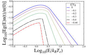
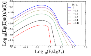
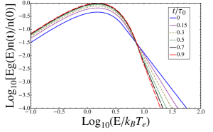
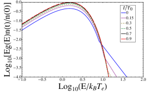
Figure 1: Evolution of $g(E,t)n(t)/n_{0}$ during the rise (upper) and decay (lower) phase for $r_{0}=4$ (left) and $8$ (right). The time unit is $\tau_{0}=l_{e}/(b_{0}v_{\rm A0})$. $C_{e}b_{i}^{4}=2b_{0}$, $S_{a}/S_{s}=100$ and $\Delta=2^{1/2}b_{0}$ for both cases.

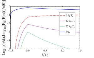
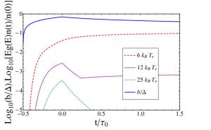
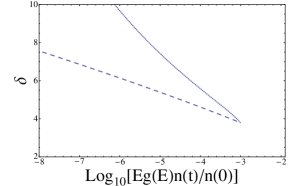
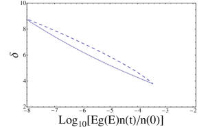
Figure 2: Evolution of $g(E,t)n(t)/n_{0}$ (upper) and correlation between $\delta$ and $g(E,t)n(t)/n_{0}$ at $E=25k_{\rm B}T_{e}$ (lower) of the evaporation models shown in Figure 1. The dashed and dotted lines in the lower panels correspond to the rise and decay phases, respectively.

The solution of equations (1) and (22) critically depends on the sign of $1-C_{e}b_{i}^{4}/2b_{0}$. For $C_{e}b_{i}^{4}=2b_{0}$ and given $b_{0}/\Delta$, $S_{a}/S_{s}$, $r_{0}$, $n_{0}$, and $T_{e}(t)=T_{e0}$, $N(E,t)$ is determined for the time in units of $\tau_{0}=l_{e}/(b_{0}v_{\rm A0})$. We will first study this simple case with $T_{e}$ remaining constant and discuss more realistic applications of the model to flare observations in the next section. For $b_{0}=2^{-1/2}\Delta$, and $S_{a}/S_{s}=100$, Figure 1 shows the evolution of $g(E,t)n(t)/n_{0}$. It is evident that, while the electron distribution is thermal and nonthermal, respectively, at low ($E\ll r_{0}k_{\rm B}T_{e}$) and high ($E\gg r_{0}k_{\rm B}T_{e}$) energies, in the intermediate energy range ($E\sim r_{0}k_{\rm B}T_{e}$) it experiences a transition from nonthermal to thermal. Moreover, the evolution of the gradual thermal component is similar for $r_{0}=4$ and $8$, in contrast to their distinct impulsive nonthermal components.

Figure 2 shows the time dependence of $g(E,t)n(t)/n_{0}$ at several energies. In combination with Figure 1, it is evident that, for the ratio of transition energy to thermal energy at the turbulence peak $r_{0}=4$, electrons at 6 $k_{\rm B}T_{e}$ are nonthermal and impulsive near the peak of $b$ and become thermal in the gradual decay phase. At $E=12$ and $25$ $k_{\rm B}T_{e}$, the distribution is nonthermal and impulsive. For $r_{0}=8$, electrons at $6\ k_{\rm B}T_{e}$ are nonthermal in the early rise phase and become part of a thermal distribution before the peak of $b$. Its sharp rise near the peak of $b$ mimics the well-known Neupert effect (Neupert, 1968). Electrons at $12\ k_{\rm B}T_{e}$ become thermal in the decay phase. Compared with the model with $r_{0}=4$, the most distinct feature is the much sharper decrease of $g$ at $E=12$ and 25 $k_{\rm B}T_{e}$ in the early decay phase. This is mostly caused by the relatively high values of $E_{t}/k_{\rm B}T_{e}$, which makes the density of nonthermal electrons very sensitive to $E_{t}$ and therefore $b(t)$ and $n(t)$.

Figure 3 shows the corresponding evolution of $\varepsilon I(\varepsilon,t)$. To increase the dynamical range of the plot, we show the energy spectrum $\varepsilon I(\varepsilon,t)$ instead of the photon number flux spectrum $I(\varepsilon,t)/\varepsilon$ normally plotted in papers on specific observations. The thin and thick lines are for the first and second term of equation (17), and the upper and lower panels are for the rise and decay phases, respectively. The distinctions between the thermal and nonthermal components are less prominent than those for electrons primarily due to the dominance of the thick-target emission and contributions of high-energy electrons to low-energy X-rays. The nonthermal HXRs are always dominated by the thick-target component, which dominates the rise phase of the $r_{0}=4$ model as well. The thin-target component only dominates the low-energy thermal emission in the late rise and decay phases. It is interesting to note that a low-energy spectral flattening in the total spectrum can result from competition between the thin- and thick-target components, which provides an alternative to the return current explanation for this observed phenomenon (Zharkova & Gordovskyy, 2006).

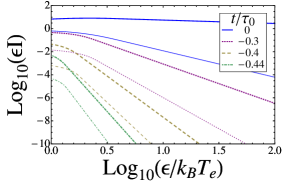
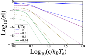
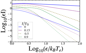
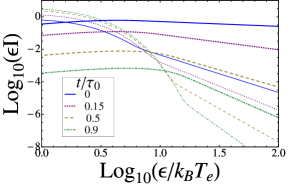
Figure 3: Evolution of the energy spectrum $\varepsilon I$ during the rise (upper) and decay (lower) phase for $r_{0}=4$ (left) and $8$ (right), where $I$ is the specific intensity rather than the photon flux, as is more often used. The unit is ${2^{3/2}\alpha e^{4}l_{0}An_{0}^{2}}(k_{\rm B}T_{e})^{1/2}/({3{\pi}m^{3/2}c^{2}R^{2}})$, where $\alpha$ is the fine structure constant and $c$ the speed of light. The thin and thick lines are for the thin- and thick-targets, respectively.

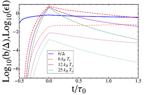
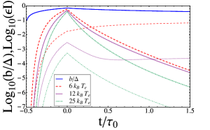
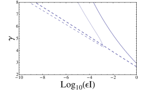
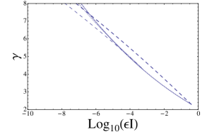
Figure 4: Light curves (upper) and correlation between differential photon flux index $\gamma$ and $\varepsilon I$ at $\varepsilon=25k_{\rm B}T_{e}$ (lower) of the evaporation models shown in Figure 3. The dashed and dotted lines in the lower panels correspond to the rise and decay phases, respectively. And the thin and thick lines are for the thin- and thick-targets, respectively.

The upper panels of Figure 4 show light curves of $\varepsilon I(\varepsilon,t)$ at several energies. The impulsive phase is mostly dominated by the thick-target emission and the thin-target component dominates in the gradual phase especially at low energies. Compared to the case with $r_{0}=4$, the HXR fluxes of $r_{0}=8$ both rise and decay more sharply with a plateau near the peak. This plateau is less distinct at higher energies. The dependence of HXRs on $r_{0}$ is a direct consequence of the dependence of the nonthermal electron density on $r_{0}$. A high value of $r_{0}$ can be caused by a low temperature and/or high density of the background electrons for a given acceleration timescale. The model therefore predicts that sharper rise and decay of HXR emission imply lower temperature and/or higher density of the thermal component. This is the key prediction of the model.

Since the evolution of $\delta(t)$ is determined by $b(t)$ (eq. [6]), the dependence of the HXR light curves on $T_{e}$ and $n$ will affect the correlation between HXR flux and differential photon spectral index $\gamma=1-{\rm d}{\rm ln}I/{\rm d}{\rm ln}\varepsilon$ frequently observed for HXR pulses (Grigis & Benz, 2004; Battaglia & Benz, 2006; Grigis & Benz, 2006, 2008). (Note that since $\gamma$ is usually defined in terms of photon number flux spectrum instead of energy flux spectrum, it differs from the index of $I$ by 1.) The lower panels of Figure 4 show how the correlation changes from the rise to decay phase at $\varepsilon=25k_{\rm B}T_{e}$. The corresponding correlation between $\delta$ and $g(E,t)n(t)/n_{0}$ is shown in the lower panels of Figure 2. Since the thick-target emission does not depend on the density of the target region, the correlation between $\delta$ and $g(E,t)n(t)$ is similar to the correlation between $\gamma$ and $\varepsilon I$. The thin-target emission scales with $n(t)^{2}g(E,t)$, and $\varepsilon I$ therefore decays more slowly than $n(t)g(E,t)$. Grigis & Benz (2004) claims that the correlation for these pulses “follows tendentially a slanted V, with the rise phase forming the flatter leg”. This is in agreement with the $r_{0}=4$ case. For higher values of $r_{0}$, our model also predicts an opposite evolution with the decay phase forming the flatter leg. Such pulses do exist (Grigis & Benz, 2008). The strongest pulse of the 25-Feb-2002 flare shown in Figure 4 of Grigis & Benz (2004) is one example. It is also interesting to note that this pulse has a relatively gradual rise and sharp decay phases in agreement with our model prediction at high energies. The majority of pulses from the 27-June-1980 flare studied by Lin & Schwartz (1987) also seems to be compatible with the latter model as shown in their Figure 8.

5 Discussion

We have shown that the model has many characteristics similar to the observed thermal and nonthermal X-ray emissions, especially for early impulsive flares (Sui et al., 2007). It also predicts that variations in properties of the thermal background plasma result in significant differences in the nonthermal particles. To test the model more quantitatively with observations, one needs to address the heating of electrons and ions and other important processes in flaring loops. The evolution of $T_{e}$ and ion temperature $T_{i}$ depends on the ill-understood plasma heating by turbulence and chromospheric evaporation. The inhomogeneity along the loops and related production of plasma waves will also affect the thermal energy gain of background particles (Zharkova & Gordovskyy, 2006; Kontar & Reid, 2009). In cases where the energy release site is localized at the looptop regions, one also needs to consider transport effects from the acceleration region to the thick-target region. Some transport processes may modify the electron distribution by inducing waves (Kontar & Reid, 2009), which may propagate into the acceleration region and affect both the acceleration and transport processes. The trapping of energetic electrons in the acceleration region also modifies the resulting photon spectral evolution (Grigis & Benz, 2006). The problem is even more complex when one considers the effect of conduction and radiation from coronal loops and chromospheric footpoints (Liu et al., 2009). For strong evaporation, shocks may form making the large-scale bulk motion an important energy component (Li et al., 2009).

There are already extensive numerical studies of the dynamics of flaring loops (Li et al., 1997; Allred et al., 2005; Klimchuk, 2006; Liu et al., 2009). Significant uncertainties remain. The essential difficulties are rooted in the highly dynamical nature of turbulent plasma in a strongly magnetized environment and we still lack effective tools to address this phenomenon in quantitative detail (Jiang et al., 2009). It is therefore not surprising that flare HXRs often show features over a broad scale range. For some flares, features from the duration of the observed HXRs down to the time resolution of the instrument can be readily identified (Aschwanden et al., 1998). Even for the relatively simple early impulsive flares with the HXRs dominated by a few distinct bursts (Sui et al., 2007; Li et al., 2009), finer structures with a timescale much shorter than the duration of individual bursts are expected (Aschwanden et al., 1996). Flare HXRs are therefore an intrinsically complex phenomenon. Detailed deductive modeling of individual flares is deemed to be tedious if possible, especially for extended bursts without distinct dominant scales.

On the other hand, for simple flares with the HXRs dominated by a few distinct bursts, which usually follow the soft-hard-soft evolution, our model can be readily applied to individual bursts to account for these energetically dominant components. The energetically less important residuals from a successful model fitting to specific flare observations can be attributed to small-scale processes ignored (or averaged out) in the model. An expansion approach in energetics therefore may be taken to achieve more and more quantitative modeling. The elementary energy events proposed here therefore may reflect more about the fact that some flares are relatively simple and may be modeled in quantitative details rather than some fundamental physical processes. If there are universal processes operating in all flares, these simple flares will be good candidates for us to disentangle these processes by modeling in detail, which may lead to interesting testable predictions. With the elementary energy release events proposed here, one can carry out detailed modeling of early impulsive events, where properties of the background electrons can be readily obtained from RHESSI’s high resolution observations of X-ray emissions. Quantitative tests of the model are possible, especially for the study of energy release during the impulsive phase when one may assume $T_{i}=T_{e}=T_{e0}$.

The energy loss needs to be treated properly to apply the model to observations especially for the gradual decay phase. To partially take into account the effect of energy loss during the impulsive phase, one may replace equation (19) with

$$\dot{n}(t)=C_{e}n_{i}[\dot{\Sigma}(t)-\Lambda]/(\rho v_{\rm A}^{2})\,,$$ (25)

where $\Lambda=\kappa_{r}n^{2}/T_{e}^{1/2}$ is the radiative cooling rate and $\kappa_{r}\simeq 1.42\times 10^{-19}$ ergs cm³ s^-1 K^1/2 (Tandberg-Hanssen & Emslie, 1988). Figure 5 shows how the density variation is reduced due to inclusion of the radiative cooling for $\Lambda_{0}/\dot{\Sigma}_{0}=0.22/b_{0}^{4}$, $C_{e}n_{i}b_{0}^{2}=2n_{0}$, and $b_{0}=1$. The density decrease for the result with radiative cooling considered may not represent observations accurately because depletion of plasmas from coronal loops produced by flares usually occurs when the plasma temperature is already so low that there are no significant X-ray emissions (Warren & Antiochos, 2004). The temperature evolution must be considered before the density reaches the peak value. This can be done when applying the model to individual flare observations.

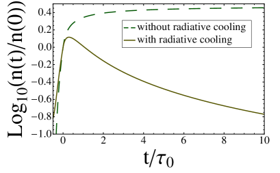
Figure 5: The evolution of the average density $n$ with (solid) and without (dashed) the radiative cooling taken into account. See text for details.

Flares associated with single loops have been studied extensively by many authors (Veronig et al., 2005; Liu et al., 2006; Sui et al., 2007; Hannah et al., 2008; Xu et al., 2008). Two flares occurring on 13-Aug-2002 after 5:30 UT are also good examples (Li et al., 2009). Among these flares, there are events with the HXR emission dominated by a single pulse (Sui et al., 2007). Our elementary energy release events can be applied to these flares directly to study all aspects of the impulsive phase. These pulses usually have a duration of less than 1 minute. It may be difficult to obtain the detailed spectral evolution, however, one can use the model to reproduce the observed light curves with a prescribed temperature evolution. $T_{e}$, $C_{e}$, and $n_{0}$ determine the thermal X-ray light curves. The photon spectral index at the HXR peak can be used to derive $b_{0}/\Delta$, which determines the evolution of the HXR spectral index. The time unit $\tau_{0}$ can be adjusted to fit the duration of the HXR pulse (Lee et al., 1995). The shape of the HXR pulse can be fitted by adjusting $S_{a}/S_{s}$ and $r_{0}$. The overall normalization $N_{0}$ depends on the size and density of the looptop acceleration region. Therefore a good fit to such flares would lead to well-defined model parameters. If observations can also give a reasonable measurement of the source size $l_{0}$, from equations (8) and (12), one can show that the model parameters $n_{0}$, $T_{e0}$, $b_{0}/\Delta$, $S_{a}/S_{s}$, $r_{0}$, $l_{0}$ must satisfy the following equation

$$r_{0}k_{\rm B}T_{e0}=(2^{5/2}\pi{\rm ln}\Lambda n_{0}l_{0}S_{a}/S_{s})^{1/2}e^{2}(\Delta/b_{0})/[(1+2S_{a}/3S_{s})^{1/2}-1]^{1/2}\,.$$ (26)

$l_{e}S_{s}$ and $l_{e}S_{a}$ are introduced in equation (3) and can be obtained in term of $\Delta$ with equations (12) and (6). The magnetic field $B$ needs to be determined from other means to get $l_{e}$ (also in term of $\Delta$) from $\tau_{0}$ and $b_{0}/\Delta$. It is evident that $\Delta$ can not be derived from the above model parameters. By replacing $\Delta$ with $l_{e}$, one, however, can express $S_{a}$ and $S_{s}$ in terms of $l_{e}$, which are intimately related to the energy release and electron interactions with the turbulence and should not change significantly from flare to flare. Of course, if the turbulence speed $b_{0}v_{\rm A}$ can also be determined through other means, one can get $l_{e}$ from $\tau_{0}$ and then derive $b_{0}$, $\Delta$, $S_{s}$, and $S_{a}$. The capability of the model to reproduce observed light curves with the constraint (26) can be considered as a test of its validity. From fitting of a large enough sample with different peak HXR spectral indexes, one may obtain statistical measurements of $C_{e}$, $l_{e}$, $b_{0}$, $\Delta$, $S_{a}$, and $S_{s}$.

There are also flares with relatively long HXR pulses ($\sim 1$ min), e.g., the 20-Sep-2002 flare starting at 9:23 UT and the flare studied in detail by Liu et al. (2006). Given the relatively gradual HXR peak of these events, the elementary energy release events will not produce a good fit to the light curves. For these events, one can obtain detailed spectral evolution. Equation (6) therefore can be used with the observed $\delta(t)$ to derive the evolution of $b(t)$ and $\Sigma(t)$ during the HXR pulses. The temperature evolution $T_{e}(t)$ can also be obtained from the spectral evolution. With $T_{e}(t)$ and $\delta(t)$ as inputs, one can again fit the observed light curves with the model to test its validity, especially the evaporation model described with equation (19). In a more accurate treatment, one should replace equation (19) with an appropriate energy conservation equation to have more insights of the evaporation and energy release processes. For more general cases, where there can be a preheating phase (Battaglia et al., 2009) and/or many HXR pulses (Veronig et al., 2005), suggesting continuous energy release, one can treat $b(t)$ as an input and apply the model to observations to derive its evolution, which can be used for further study of plasma heating, particle acceleration, and chromospheric evaporation.

6 Conclusions

Although the particle acceleration timescale is short, the energy release processes of solar flares are multi-scale phenomena and some long timescale processes may have imprints on the characteristics of nonthermal components. In this paper, we demonstrate how the evolution of X-ray emissions may be affected by the chromospheric evaporation in the context of stochastic acceleration by turbulent electromagnetic fields. We consider the simplest scenario, where the energy release in closed loops is described with a turbulence intensity $b_{0}B$ and generation scale $l_{e}$. It is shown that the HXR flux has a sharper decay phase for events with lower temperature and/or higher density of the background electrons, which makes the transition energy between the thermal and nonthermal component much higher than $k_{\rm B}T_{e}$. As the ratio, $r_{0}$, of the transition energy to the thermal energy at the HXR peak is varied from low to high values (by varying the density and temperature) the HXR behaviour changes between two types of spectral evolution. If this ratio is low, the flux change in the rise phase is higher than in the decay phase for a given change in the spectral index (the commonly observed behaviour) and vice versa if $r_{0}$ is high — a behaviour which is also observed, though less frequently.

Solar flares involve many physical processes that give rise to significant uncertainties in our understanding of the plasma heating and particle acceleration. Even for relatively simple flares associated with single loops, the mass, momentum, and energy transport along the loops during the impulsive phase can be highly dynamical and complicated. It is therefore challenging to study the flare energy release with all the relevant processes treated properly. The problem can be simplified significantly if we are mostly concerned with the energetically dominant processes such as the energy release, particle acceleration, and chromospheric evaporation averaged over a relatively long timescale of observational interest. We discuss how the model may be applied to RHESSI observations of flares for quantitative investigations, especially for early impulsive flares with the HXRs dominated by a single pulse with soft-hard-soft spectral evolution.

While the short acceleration timescale may suggest microscopic processes, the large amount of energy released during flares reveals a predominantly macroscopic process. One critical aspect of solar flare studies is to understand the connection between the microscopic particle acceleration and the macroscopic energy release. The latter has been studied with magnetohydrodynamical simulations. The study of particle acceleration is limited to a few very specific mechanisms. Although the high degree of freedom on large scales (in connection with the magnetic field configuration and initial and boundary conditions) inevitably lead to multi-scale features giving rise to significant complexities, the small scale processes are expected to follow some patterns as least in a statistical sense. One therefore may focus on flares with relatively simple HXR light curves. The model presented here makes it possible to infer the energy release rate from the observed HXR emission for these flares. It is therefore possible to probe the macroscopic energy release processes with the impulsive nonthermal emission. Successful applications of the model to flare observations will lead to quantitative measurements of the particle acceleration and scattering rate by turbulent electromagnetic fields. The obtained $b(t)$ can be compared with MHD simulations of flares or models of large scale energy release processes for more quantitative and self-consistent modeling.

References

- Allred et al. (2005) Allred, J. C., Hawley, S. L., Abbett, W. P., & Carlsson, M. 2005, ApJ, 630, 573
- Antiochos & Sturrock (1978) Antiochos, S. K., & Sturrock, P. A. 1978, ApJ, 220, 1137
- Aschwanden (2002) Aschwanden, M. J. 2002, Space Science Reviews, 101, 1
- Aschwanden et al. (1996) Aschwanden, M. J., Hudson, H., Kosugi, T., & Schwartz, R. A. 1996, ApJ, 464, 985
- Aschwanden et al. (1998) Aschwanden, M. J., Schwartz, R. A., & Dennis, B. R. 1998, ApJ, 502, 468
- Battaglia & Benz (2006) Battaglia, M., & Benz, A. O. 2006, A&A, 456, 751
- Battaglia et al. (2009) Battaglia, M., Fletcher, L., & Benz, A. O. 2009, A&A, 498, 901
- Benz (1977) Benz, A. O. 1977, ApJ, 211, 270
- Bethe & Heitler (1934) Bethe, H. A., & Heitler, W. 1934, Proc. Roy. Soc. (London), A146, 83
- Brown (1973) Brown, J. C. 1973, Solar Phys. 31, 143
- Brown & Melrose (1977) Brown, J. C., & Melrose, D. B. 1977, Solar Phys. 52, 117
- Brown et al. (2009) Brown, J. C., Turkmani, R., Kontar, E. P., MacKinnon, A. L., & Vlahos, L. 2009, A&A, in press, astro-ph/0909.4243.
- Bykov & Fleishman (2009) Bykov, A. M., & Fleishman, G. D. 2009, ApJ, 692, L45
- De Jager & De Jonge (1978) De Jager, C., & De Jonge, G. 1978, Solar. Phys., 58, 127
- Drake et al. (2006) Drake, J. F., Swisdak, M., Che, H., & Shay, M. A. 2006, Nature, 443, 553
- Fletcher & Hudson (2008) Fletcher, L., & Hudson, H. S. 2008, ApJ, 675, 1645
- Galloway et al. (2005) Galloway, R. K., MacKinnon, A. L., Kontar, E. P., & Helander, P. 2005, A&A, 438, 1107
- Grigis & Benz (2004) Grigis, P. C., & Benz, A. O. 2004, A&A, 426, 1093
- Grigis & Benz (2006) Grigis, P. C., & Benz, A. O. 2006, A&A, 458, 641
- Grigis & Benz (2008) Grigis, P. C., & Benz, A. O. 2008, A&A, 683, 1180
- Haerendel (2009) Haerendel, G. 2009, ApJ, In press.
- Hamilton & Petrosian (1992) Hamilton, R. J., & Petrosian, V. 1992, ApJ, 398, 350
- Hannah et al. (2008) Hannah, I. G., Krucker, S., Hudson, H. S., Christe, S., & Lin, P. R. 2008, A&A, 481, L45
- Holman (1985) Holman, G. D. 1985, ApJ, 293, 584
- Hoyng et al. (1976) Hoyng, P., Brown, J. C., & Van Beek, H. F. 1976, Solar Phys. 48, 197
- Jiang et al. (2006) Jiang, Y. W., Liu, S., Liu, W., & Petrosian, V. 2006, ApJ, 638, 1140
- Jiang et al. (2009) Jiang, Y. W., Liu, S., & Petrosian, V. 2009, ApJ, 698, 163
- Klimchuk (2006) Klimchuk, J. A. 2006, Solar Phys., 234, 41
- Kontar & Reid (2009) Kontar, E. P., & Reid, H. A. S. 2009, ApJ, 695, L140
- Kraichnan (1965) Kraichnan, R. H. 1965, Phys. of Fluids, 8, 1385
- Krucker et al. (2008) Krucker, S., Hurford, G. J., MacKinnon, A. L., Shih, A. Y., & Lin, P. R. 2008, ApJ 678, L63
- Krucker et al. (2008) Krucker, S., et al. 2008, A&A Rev. 16, 155
- Krucker et al. (2009) Krucker, S., et al. 2009, ApJ, Submitted.
- Lee et al. (1995) Lee, T. T., Petrosian, V., & McTiernan, J. M. 1995, ApJ, 448, 915
- Li et al. (1997) Li, P., McTiernan, J. M., & Emslie, A. G. 1997, ApJ, 491, 395
- Li et al. (2009) Li, Y. P., Gan, W. Q., & Su, Y. 2009, Research in A&A, 9, 1155
- Lin & Schwartz (1987) Lin, R. P., & Schwartz, R. A. 1987, ApJ, 312, 462.
- Liu et al. (2006) Liu, W,, Liu, S, Jiang, Y. W., & Petrosian, V. 2006, ApJ, 649, 1124
- Liu & Fletcher (2009) Liu, S., & Fletcher, L. 2009, ApJ, 701, L34
- Liu et al. (2009) Liu, W., Petrosian, V., & Mariska, J. T. 2009, ApJ, 702, 1553
- Miller & Roberts (1995) Miller, J. A., & Roberts, D. A. 1995, ApJ, 452, 912
- Miller et al. (1997) Miller, J. A., et al. 1997, J. Geophys. Res. 102, 14631
- Neupert (1968) Neupert, W. M. 1968, ApJ, 153, L59
- Petrosian & Donaghy (1999) Petrosian, V., & Donaghy, T. Q. 1999, ApJ, 527, 945
- Petrosian & Liu (2004) Petrosian, V., & Liu, S. 2004, ApJ, 10, 550
- Shao & Huang (2009) Shao, C. W., & Huang, G. L. 2009, ApJ, 694, L162
- Sui et al. (2007) Sui, L. H., Holman, G. D., & Dennis, B. R. 2007, ApJ, 670, 862
- Tandberg-Hanssen & Emslie (1988) Tandberg-Hanssen, E., & Emslie, G. 1988, The Physics of Solar Flares (Cambridge: Cambridge Univ. Press)
- Tsuneta & Naito (1998) Tsuneta, S., & Naito, T. 1998, ApJ, 495, L67
- Van Beek et al. (1974) Van Beek, H. F., De Feiter, L. D., & De Jager, C. 1974, Space Research XIV, 447
- Veronig et al. (2005) Veronig, A. M., et al. 2005, ApJ, 621, 482
- Warren & Antiochos (2004) Warren, H. P., & Antiochos, S. K. 2004, ApJ, 611, L49
- Xu et al. (2008) Xu, Y., Emslie, A. G., & Hurford, G. J. 2008, ApJ, 673, 576
- Zharkova & Gordovskyy (2006) Zharkova, V. V., & Gordovsky, M. 2006, ApJ, 651, 553