Bogoliubov Theory and Lee-Huang-Yang Corrections in Spin-1 and Spin-2 Bose-Einstein Condensates in the Presence of the Quadratic Zeeman Effect

Abstract

We develop Bogoliubov theory of spin-1 and spin-2 Bose-Einstein condensates (BECs) in the presence of a quadratic Zeeman effect, and derive the Lee-Huang-Yang (LHY) corrections to the ground-state energy, pressure, sound velocity, and quantum depletion. We investigate all the phases of spin-1 and spin-2 BECs that can be realized experimentally. We also examine the stability of each phase against quantum fluctuations and the quadratic Zeeman effect. Furthermore, we discuss a relationship between the number of symmetry generators that are spontaneously broken and that of Nambu-Goldstone (NG) modes. It is found that in the spin-2 nematic phase there are special Bogoliubov modes that have gapless linear dispersion relations but do not belong to the NG modes.

I Introduction

The Bogoliubov theory of weakly-interacting Bose-Einstein condensates (BECs) bogoliubov has served as an indispensable tool in diverse subfields of physics. For a scalar BEC of bosons with mass $M$, particle-number density $n$, and $s$-wave scattering length $a$, the ground-state energy (GSE) of the system with volume $V$ is given by

$$E_{0}=\frac{2\pi\hbar^{2}Vn^{2}}{M}a\left(1+\frac{128}{15}\sqrt{\frac{na^{3}}{\pi}}+\cdots\right),$$ (1)

where the first term on the right-hand side is the mean-field energy, the second term gives a nonperturbative correction to it which was first derived by Lee, Huang, and Yang (LHY) lee ; lhy , and the higher-order terms were discussed in Refs. wu ; hugenholtz ; sawada . In the present paper, we discuss Bogoliubov theory and LHY corrections of BECs with spin degrees of freedom in the presence of a quadratic Zeeman effect.

The Bogoliubov theory of spinor BECs has been discussed extensively over the past decade. The spin-1 Bogoliubov spectra have been derived in Refs. ho ; ohmi ; huang ; ueda2 up to the linear Zeeman effect. In Ref. szirmai , the same problem is discussed from a field-theoretic point of view. The effect of the quadratic Zeeman energy on the spin-1 BEC has been discussed in Refs. murata ; ruostekoski . The spin-2 BEC has been examined in the absence of an external magnetic field in Ref. suominen and up to the linear Zeeman effect in Ref. ueda . However, little attention has been paid to the GSEs.

In this paper, we develop a systematic renormalization procedure and derive GSEs, pressure, sound velocity, and quantum depletion up to the LHY corrections. The LHY corrections have been measured for a scalar BEC xu ; papp and for a two-component Fermi gas grimm by using methods to enhance quantum fluctuations. The experiment in Ref. xu utilized a strongly correlated system in an optical lattice, while the experiments in Refs. papp ; grimm amplified the coupling constant by means of a Feshbach resonance. Our analysis takes into account the quadratic Zeeman effect that is of great importance under many experimental situations in which the linear Zeeman effect can be ignored. Because the sign of the quadratic Zeeman term $q$ can be manipulated experimentally leslie , both cases of positive and negative $q$ are analyzed. It is shown that except for the ferromagnetic phase the LHY correction in a spinor BEC is affected by the quadratic Zeeman effect and that it can be measured by making strongly correlated systems or by controlling the external magnetic field.

The order parameter of a spin-2 nematic BEC in the absence of an external magnetic field depends on an additional parameter, $\eta$, that is not related to the symmetry of the Hamiltonian but describes the degeneracy between the uniaxial and biaxial nematic phases. As pointed out in Refs. turner ; song , however, quantum fluctuations induce a quantum phase transition between the two phases, lifting the degeneracy. We show that the quadratic Zeeman effect with $q<0$ causes the dynamical instability in the uniaxial nematic phase, whereas it leaves the biaxial nematic phase stable. That is, the uniaxial nematic phase is unstable against an infinitesimal negative quadratic Zeeman effect in the thermodynamic limit. Conversely, the quadratic Zeeman effect with $q>0$ makes the biaxial nematic phase dynamically unstable while it leaves the uniaxial nematic phase stable. However, it is possible to stabilize both of these phases for nonzero $q$ in a finite system. We will show this for the case of a spin-2 BEC.

The Bogoliubov theory predicts massless modes, which can be interpreted as Nambu-Goldstone (NG) modes associated with spontaneous symmetry breaking. To elucidate this point, we discuss a relationship between the number of symmetry generators that are spontaneously broken and the number of NG modes nielsen . We apply the relationship to spin-1 and spin-2 BECs, and point out that for the uniaxial and biaxial nematic phases there exist the Bogoliubov modes that have gapless linear dispersion relations but do not belong to the NG modes.

This paper is organized as follows. Section II formulates the problem, and describes the low-energy Hamiltonian and Hartree-Fock approximation of a spin-$f$ BEC. Section III discusses the problem of divergence of the GSE and how to remove the divergence by renormalization of the coupling constant. Sections IV and V examine the mean-field phase diagrams and Bogoliubov theory of spin-1 and spin-2 BECs, respectively, in the thermodynamic limit, and derive the Bogoliubov spectra and LHY corrections. Section VI discusses the relationship between the number of symmetry generators that are spontaneously broken and the number of NG modes in spinor BECs. Section VII provides the summary and concluding remarks. The detailed derivations of the GSEs are described in Appendix A, and the properties and equation numbers of the physical quantities in each phase and notations are listed in Appendix B.

II Formulation of the problem

We consider a system of $N$ spin-$f$ identical bosons with mass $M$ that undergo an $s$-wave scattering subject to periodic boundary conditions. As in most experiments done in spinor BECs, we consider the case in which the linear Zeeman effect can be ignored. Let $\displaystyle\hat{\Psi}_{m}(\mathbf{x})$ $(m=-f,-f+1,...,f)$ be the field operator of a boson at position $\displaystyle\mathbf{x}$ with magnetic quantum number $m$, where we assume that an external magnetic field $B$ is applied in the $z$ direction. Then, the low-energy effective Hamiltonian of a spin-$f$ BEC is given by

$$\hat{H}=\hat{H}_{\text{KE}}+\hat{H}_{\text{QZ}}+\hat{V},$$ (2)

where

$$\hat{H}_{\text{KE}}=\int d\mathbf{x}\ \hat{\Psi}^{\dagger}_{m}(\mathbf{x})\Big{(}-\frac{\hbar^{2}\nabla^{2}}{2M}\Big{)}\hat{\Psi}_{m}(\mathbf{x})$$ (3)

is the kinetic energy,

$$\hat{H}_{\text{QZ}}=qm^{2}\int d\mathbf{x}\ \hat{\Psi}^{\dagger}_{m}(\mathbf{x})\hat{\Psi}_{m}(\mathbf{x})$$ (4)

is the quadratic Zeeman term, and

$$\hat{V}=\sum_{F=0}^{2f}\frac{\bar{g}_{F}}{2}\sum_{M=-F}^{F}\langle fmfm^{\prime}|FM\rangle\langle FM|f\mu f\mu^{\prime}\rangle\int d\mathbf{x}\ \hat{\Psi}_{m}^{\dagger}(\mathbf{x})\hat{\Psi}_{m^{\prime}}^{\dagger}(\mathbf{x})\hat{\Psi}_{\mu}(\mathbf{x})\hat{\Psi}_{\mu^{\prime}}(\mathbf{x})$$ (5)

is the interaction energy. The strength of the quadratic Zeeman term is given by $q=(g\mu_{B}B)^{2}/E_{\text{hf}}$, where $g$ is the Landé $g$-factor, $\mu_{B}$ is the Bohr magneton, and $E_{\text{hf}}$ is the hyperfine energy splitting. In Eq. (5), $\bar{g}_{F}$ is a bare coupling constant in the total spin $F$ channel and $\displaystyle\langle fmfn|FM\rangle$ is the Clebsch-Gordan coefficient. Here and henceforth, repeated indices such as $m,m^{\prime},\mu,\ \text{and}\ \mu^{\prime}$ are assumed to be summed over $f,f-1,...,-f$ unless otherwise stated. Bose symmetry requires that the total spin $F$ in the $s$-wave channel is even. In fact, it follows from the canonical commutation relations of bosons and the properties of the Clebsch-Gordan coefficients that the terms in Eq. (5) with odd $F$ vanish identically.

We expand the field operator as

$$\hat{\Psi}_{m}(\mathbf{x})=\frac{1}{\sqrt{V}}\sum_{\mathbf{k}}\hat{a}_{\mathbf{k},m}\text{e}^{i\mathbf{k\cdot x}},$$ (6)

where $V$ is the volume of the system and $\hat{a}_{\mathbf{k},m}$ is the annihilation operator of a spin-$f$ boson with wave number $\mathbf{k}$ and magnetic quantum number $m$. Substituting Eq. (6) in Eq. (2), we obtain

$$\hat{H}=\sum_{\mathbf{k}}(\epsilon_{\mathbf{k}}+qm^{2})\hat{a}^{\dagger}_{\mathbf{k},m}\hat{a}_{\mathbf{k},m}+\sum_{F=0}^{2f}\frac{\bar{g}_{F}}{2V}\sum_{M=-F}^{F}\sum_{\mathbf{k},\mathbf{p},\mathbf{q}}\langle fmfm^{\prime}|FM\rangle\langle FM|f\mu f\mu^{\prime}\rangle\hat{a}_{\mathbf{p},m}^{\dagger}\hat{a}_{\mathbf{q},m^{\prime}}^{\dagger}\hat{a}_{\mathbf{p+k},\mu}\hat{a}_{\mathbf{q-k},\mu^{\prime}},$$ (7)

where $\epsilon_{\mathbf{k}}=\hbar^{2}\mathbf{k}^{2}/2M$.

In the mean-field or Hartree-Fock approximation, all bosons are assumed to occupy a single mode, which we label as $\mathbf{0}$:

$$|\mathbf{\zeta}\rangle=\frac{1}{\sqrt{N!}}\left(\sum_{m=-f}^{f}\zeta_{m}\hat{a}^{\dagger}_{\mathbf{0},m}\right)^{N}|\text{vac}\rangle,$$ (8)

where variational parameters $\zeta_{m}$ are assumed to satisfy the normalization condition $\sum_{m}|\zeta_{m}|^{2}=1$ and they are determined so as to minimize the expectation value of the Hamiltonian. By using the trial state (8), it is possible to classify the mean-field ground-state phase in a number-conserving manner ueda2 ; koashi ; ueda .

III Renormalization of the ground-state energy

If we take into account the effects of quantum fluctuations, physical quantities such as GSE show ultraviolet divergence. This divergence stems from use of the contact interaction, which gives correct results if we only consider the region $|\mathbf{x}|\gg r_{0}$, where $r_{0}$ is the range of the interaction. This implies that the effective Hamiltonian (2) is only valid below a certain cutoff momentum. By introducing the cutoff, the GSE no longer diverges but depends explicitly on the cutoff. The renormalization of the coupling constant eliminates the cutoff in favor of an observable, that is, an $s$-wave scattering length in the present problem.

To examine this problem of the coupling constant in detail, let us first consider the low-energy scattering between spin-$f$ identical bosons. The scattering rate for each scattering channel is determined by the $T$-matrix $\hat{T}$, which is the solution to the following equation pethick :

$$\hat{T}=\hat{V}+\hat{V}\frac{1}{E-2\hat{H}_{\text{KE}}}\hat{T},$$ (9)

where $E$ is the total energy and $1/(E-2\hat{H}_{\text{KE}})$ is the two-particle Green’s function. We deal with the quadratic Zeeman term perturbatively by assuming that it is at most of the order of $\hat{V}$ – the condition well satisfied in current experiments. This assumption is implicitly made in classifying the mean-field ground-state phases in Refs. murata ; stenger ; saito .

The $T$-matrix is related to the $s$-wave scattering lengths $a_{F}$ and renormalized coupling constants $g_{F}$ as follows:

$$g_{F}\equiv\frac{4\pi\hbar^{2}a_{F}}{M}=\lim_{k\to 0}\langle\mathbf{k^{\prime}},F|\hat{T}|\mathbf{k},F\rangle,$$ (10)

where $\mathbf{k}$ and $\mathbf{k^{\prime}}$ are the incoming and outgoing wave vectors, respectively, and $k\equiv|\mathbf{k}|=|\mathbf{k^{\prime}}|$ because of energy conservation. In the Hartree-Fock approximation, the $T$-matrix is approximated by $\hat{T}\approx\hat{V}$, and therefore

$$g_{F}\equiv\frac{4\pi\hbar^{2}a_{F}}{M}=\bar{g}_{F}.$$ (11)

In the Bogoliubov theory, however, this approximation does not remove the cutoff dependence because the divergence occurs at the level of second order in $\bar{g}_{F}$. Thus, we must approximate the $T$-matrix up to second order in the coupling constants:

$$\hat{T}\approx\hat{V}+\hat{V}\frac{1}{E-2\hat{H}_{\text{KE}}}\hat{V}.$$ (12)

The corresponding relation between the bare and renormalized coupling constants is given by

$$g_{F}\equiv\frac{4\pi\hbar^{2}a_{F}}{M}=\bar{g}_{F}-\frac{\bar{g}_{F}^{2}}{V}{\sum_{\mathbf{k}}}^{{}^{\prime}}\frac{1}{2\epsilon_{\mathbf{k}}},$$ (13)

where the prime on the sum means to omit the term $\mathbf{k}=\mathbf{0}$. The diagrammatic representation of Eq. (13) is shown in Fig. 1.

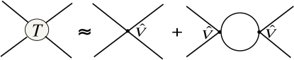
Figure 1: Diagrammatic representation of the coupling-constant renormalization in Eq. (13), where each solid line describes the one-particle Green’s function of the Hamiltonian $\hat{H}_{\text{KE}}$ and each vertex represents $\hat{V}$. The first diagram on the right-hand side represents the Hartree-Fock term, and the second diagram represents the second-order term.

Next, we illustrate how this renormalization of the coupling constant eliminates the cut-off dependence. As we will show in subsequent sections, the GSE in the absence of an external magnetic field is expressed as

$$E_{0}=E_{0}^{\text{MF}}+E_{0}^{\text{QF}}.$$ (14)

Here $E_{0}^{\text{MF}}$ is the mean-field energy

$$E_{0}^{\text{MF}}=\frac{Vn^{2}\bar{C}}{2},$$ (15)

where $n=N/V$, and $\bar{C}$ is a linear combination of the bare coupling constants. The term $E_{0}^{\text{QF}}$ in Eq. (14) describes the contribution from quantum fluctuations around the Hartree-Fock mean field and takes the following form:

$$E_{0}^{\text{QF}}=-\frac{\hbar^{2}}{4M}\sum_{j}{\sum_{\mathbf{k}}}^{{}^{\prime}}\Bigg{[}k^{2}+\frac{2Mn\bar{C}_{j}}{\hbar^{2}}-k\sqrt{k^{2}+\frac{4Mn\bar{C}_{j}}{\hbar^{2}}}\Bigg{]},$$ (16)

where the sum over $j$ is taken over the Bogoliubov modes, each of which describes fluctuations such as density and spin fluctuations, and $\bar{C}_{j}$ is a linear combination of the bare coupling constants. At the limit of $k\to\infty$, the integrand behaves as follows:

$$k^{2}+\frac{2Mn\bar{C}_{j}}{\hbar^{2}}-k\sqrt{k^{2}+\frac{4Mn\bar{C}_{j}}{\hbar^{2}}}\xrightarrow[k\to\infty]{}\frac{1}{2}\left(\frac{2MnC_{j}}{\hbar^{2}k}\right)^{2}+O\left(\frac{1}{k^{4}}\right),$$ (17)

where we substitute a renormalized coupling constant $C_{j}$ for $\bar{C}_{j}$ on the right-hand side, which is correct up to the second order in the coupling constants. On the other hand, from the $T$-matrix calculation of Eq. (13) (note that $g_{F}$ and $\bar{g}_{F}$ correspond to $C$ and $\bar{C}$, respectively), the mean-field energy is calculated to give

$$E_{0}^{\text{MF}}=\frac{Vn^{2}C^{2}}{2}+\frac{\hbar^{2}}{8M}\sum_{j}{\sum_{\mathbf{k}}}^{{}^{\prime}}\left(\frac{2MnC_{j}}{\hbar^{2}k}\right)^{2}.$$ (18)

Here the second term on the right-hand side cancels the ultraviolet part of Eq. (16). Thus, the cutoff dependence of $E_{0}^{\text{QF}}$ is removed. Therefore, the GSE is given by

$$E_{0} = \frac{Vn^{2}C}{2}-\frac{\hbar^{2}}{4M}\sum_{j}{\sum_{\mathbf{k}}}^{{}^{\prime}}\Bigg{[}k^{2}+\frac{2MnC_{j}}{\hbar^{2}}-k\sqrt{k^{2}+\frac{4MnC_{j}}{\hbar^{2}}}-\frac{1}{2}\left(\frac{2MnC_{j}}{\hbar^{2}k}\right)^{2}\Bigg{]}$$ (19)

$$= \frac{Vn^{2}C}{2}-\frac{\hbar^{2}}{8\pi^{2}M}\sum_{j}\left(\frac{2MnC_{j}}{\hbar^{2}}\right)^{\frac{5}{2}}\int_{x_{j}}^{\infty}dx\ x^{2}\left(x^{2}+1-x\sqrt{x^{2}+2}-\frac{1}{2x^{2}}\right)$$

$$\simeq \frac{Vn^{2}C}{2}\Bigg{(}1+\frac{16\sqrt{M^{3}}}{15\hbar^{3}\pi^{2}}\sum_{j}\frac{C_{j}}{C}\sqrt{nC_{j}^{3}}\Bigg{)},$$

where $x_{j}\equiv 2\pi\hbar/(V^{1/3}\sqrt{2MnC_{j}})$, and we take the thermodynamic limit $x_{j}=0$ to obtain the last expression. Even if we incorporate the quadratic Zeeman effect, the above cancellation mechanism holds as shown in Appendix A.

IV Spin-1 BEC

For a spin-1 BEC, the total spin $F$ of two interacting bosons must be 0 or 2, and therefore, Eq. (7) reduces to

$$\hat{H}=\sum_{\mathbf{k}}(\epsilon_{\mathbf{k}}+qm^{2})\hat{a}^{\dagger}_{\mathbf{k},m}\hat{a}_{\mathbf{k},m}+\frac{1}{2V}\sum_{\mathbf{k},\mathbf{p},\mathbf{q}}\Bigg{(}\bar{c}_{0}^{(1)}\hat{a}_{\mathbf{p},m}^{\dagger}\hat{a}_{\mathbf{q},m^{\prime}}^{\dagger}\hat{a}_{\mathbf{p+k},{m}}\hat{a}_{\mathbf{q-k},{m^{\prime}}}$$

$$+\bar{c}_{1}^{(1)}\mathbf{f}_{mm^{{}^{\prime}}}\cdot\mathbf{f}_{\mu\mu^{\prime}}\hat{a}_{\mathbf{p},m}^{\dagger}\hat{a}_{\mathbf{q},\mu}^{\dagger}\hat{a}_{\mathbf{p+k},{m^{{}^{\prime}}}}\hat{a}_{\mathbf{q-k},\mu^{\prime}}\Bigg{)},$$ (20)

where $\bar{c}_{0}^{(1)}=(\bar{g}_{0}+2\bar{g}_{2})/3,$ $\bar{c}_{1}^{(1)}=(\bar{g}_{2}-\bar{g}_{0})/3,$ and $\mathbf{f}_{mm^{\prime}}=(f^{x}_{mm^{\prime}},f^{y}_{mm^{\prime}},f^{z}_{mm^{\prime}})$ represents a set of the spin-1 matrices given by

$${f}^{x}=\frac{1}{\sqrt{2}}\begin{pmatrix}0&1&0\\ 1&0&1\\ 0&1&0\end{pmatrix},\ \ {f}^{y}=\frac{i}{\sqrt{2}}\begin{pmatrix}0&-1&0\\ 1&0&-1\\ 0&1&0\end{pmatrix},\ \ {f}^{z}=\begin{pmatrix}1&0&0\\ 0&0&0\\ 0&0&-1\end{pmatrix}.$$ (21)

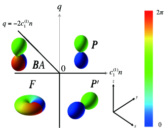
Figure 2: (Color online) Phase diagram of spin-1 BECs, where F, P (P’), and BA stand for the ferromagnetic, polar, and broken-axisymmetry phases, respectively. The spinor order parameters $(\zeta_{1},\zeta_{0},\zeta_{-1})$ of P and P’ are given by $(0,1,0)$ and $(1/\sqrt{2},0,1/\sqrt{2})$, respectively, which are transformed each other by a $\pi/2$ rotation about the $x$ axis. The degeneracy of these states are lifted by the quadratic Zeeman effect. The thick lines represent the phase boundaries. The shape of the wave function in each phase is calculated in terms of polar angle $\theta$ and azimuthal angle $\phi$ as $|\Psi(\theta,\phi)|^{2}\equiv|\sum_{m}\zeta_{m}\text{Y}_{1}^{m}(\theta,\phi)|^{2}$, where $Y^{m}_{1}(\theta,\phi)$ $(m=1,0,-1)$ are the spherical harmonics of rank 1 and color represents the phase of $\Psi(\theta,\phi)$ (see the right color gauge). The axes of the spin coordinates are shown at the bottom right of the phase diagram.

The possible phases and phase boundaries of spin-1 BEC are shown in Fig. 2 and described as follows stenger ; murata :

$$\text{ferromagnetic phase:}\ \ \ q<0,\ \ c_{1}^{(1)}<0,\ \ \text{and}\ \ \mathbf{\zeta}^{F}=(1,0,0),$$ (22)

$$\text{polar phase:}\ \ \ q>0,\ \ q>-2c_{1}^{(1)}n,\ \ \text{and}\ \ \mathbf{\zeta}^{P}=(0,1,0),$$ (23)

$$\ \ \ \ \ \ \ \ \ \ \ \ \ \ \ \ \ \ \ \ q<0,\ \ c_{1}^{(1)}>0,\ \ \ \text{and}\ \ \mathbf{\zeta}^{P^{\prime}}=\frac{1}{\sqrt{2}}(1,0,1),$$ (24)

$$\text{broken-axisymmetry phase:}\ \ \ q>0,\ \ c_{1}^{(1)}<0,\ \ q<-2c_{1}^{(1)}n,\ \ \text{and}\ \ \mathbf{\zeta}^{BA}=\left(\frac{\sin\theta}{\sqrt{2}},\cos\theta,\frac{\sin\theta}{\sqrt{2}}\right),$$ (25)

where $c_{0}^{(1)}=(g_{0}+2g_{2})/3$, $c_{1}^{(1)}=(g_{2}-g_{0})/3$, $\sin\theta=\sqrt{1/2+q/(4nc_{1}^{(1)})}$. In Fig. 2, the shape and color of the wave function in each phase represent the symmetry of the order parameter. For example, the spinor of the polar phase, $\zeta^{P}$ has a rotational symmetry about the $z$ axis, since the shape and color are symmetric about the same axis. The ferromagnetic phase apparently does not have an axisymmetry because the color changes around the $z$ axis. However, the $U(1)$ gauge transformation can make up for the variation of the color so that due to the spin-gauge symmetry, the ferromagnetic phase maintains the $U(1)$ symmetry. The broken-axisymmetry phase does not possess any continuous symmetry because any $U(1)\times SO(2)$ transformations cannot compensate for the variation of the color shown.

The ferromagnetic phase has a longitudinal magnetization, whereas the broken-axisymmetry phase has a transverse one that depends on $q$. Moreover, the broken-axisymmetry phase has a finite spin-singlet pair amplitude that also depends on $q$. In contrast, both spinors of P and P’ have no magnetization but a finite spin-singlet pair amplitude that is independent of $q$. These properties in each phase are summarized in Appendix B. Since $c_{1}^{(1)}>0$, the spin-1 ²³Na condensate is in the polar phase. On the other hand, since $c_{1}^{(1)}<0$, the spin-1 ⁸⁷Rb condensates can be in any of the ferromagnetic, broken-axisymmetry, and polar phases, depending on the sign and magnitude of $q$.

In the Bogoliubov theory, we replace operators $\hat{a}_{\mathbf{0},m}$ by c-numbers $\sqrt{N_{0}}\zeta_{m}$ and keep $\hat{a}^{\dagger}_{\mathbf{k}\neq 0,m}$ and $\hat{a}_{\mathbf{k}\neq 0,m}$ up to the second order in the Hamiltonian, where $N_{0}$ is the number of condensate bosons, which, together with $\displaystyle\hat{n}_{\mathbf{k},m}\equiv\hat{a}^{\dagger}_{\mathbf{k},m}\hat{a}_{\mathbf{k},m}$, satisfies

$$N_{0}+{\sum_{\mathbf{k}}}^{{}^{\prime}}\sum_{m}\hat{n}_{\mathbf{k},m}=N,$$ (26)

where $N$ is the total number of bosons. The Bogoliubov Hamiltonian of a spin-1 BEC is thus given by ueda2 ; murata

$$\hat{H}_{\text{eff}} = \frac{Vn^{2}}{2}\left(\bar{c}_{0}^{(1)}+\bar{c}_{1}^{(1)}\langle\mathbf{f}\rangle^{2}\right)+qN\langle(f^{z})^{2}\rangle+{\sum_{\mathbf{k}}}^{{}^{\prime}}\Bigg{[}\left(\epsilon_{\mathbf{k}}-nc_{1}^{(1)}\langle\mathbf{f}\rangle^{2}+qm^{2}-q\langle(f^{z})^{2}\rangle\right)\hat{a}^{\dagger}_{\mathbf{k},m}\hat{a}_{\mathbf{k},m}$$ (27)

$$+nc_{1}^{(1)}\langle\mathbf{f}\rangle\cdot\mathbf{f}_{mm^{\prime}}\hat{a}^{\dagger}_{\mathbf{k},m}\hat{a}_{\mathbf{k},m^{\prime}}+\frac{nc_{0}^{(1)}}{2}\left(2\hat{D}_{\mathbf{k}}^{\dagger}\hat{D}_{\mathbf{k}}+\hat{D}_{\mathbf{k}}\hat{D}_{\mathbf{-k}}+\hat{D}_{\mathbf{k}}^{\dagger}\hat{D}_{\mathbf{-k}}^{\dagger}\right)$$

$$+\frac{nc_{1}^{(1)}}{2}\left(2\mathbf{\hat{F}}_{\mathbf{k}}^{\dagger}\cdot\mathbf{\hat{F}}_{\mathbf{k}}+\mathbf{\hat{F}}_{\mathbf{k}}\cdot\mathbf{\hat{F}}_{\mathbf{-k}}+\mathbf{\hat{F}}_{\mathbf{k}}^{\dagger}\cdot\mathbf{\hat{F}}_{\mathbf{-k}}^{\dagger}\right)\Bigg{]},$$

where

$$\langle\mathbf{f}\rangle\equiv\sum_{m,m^{\prime}}\mathbf{f}_{mm^{\prime}}\zeta_{m}^{*}\zeta_{m^{\prime}},$$ (28)

$$\hat{D}_{\mathbf{k}}\equiv\sum_{m}\zeta^{*}_{m}\hat{a}_{\mathbf{k},m},$$ (29)

$$\mathbf{\hat{F}}_{k}\equiv\sum_{m,m^{\prime}}\mathbf{f}_{mm^{\prime}}\zeta^{*}_{m}\hat{a}_{\mathbf{k},m^{\prime}}.$$ (30)

Here, $\hat{D}_{\mathbf{k}}$ and $\hat{\mathbf{F}}_{\mathbf{k}}$ denote the density and spin fluctuation operators of the condensate, respectively. In Eq. (27), we substitute $c_{i}^{(1)}$ for $\bar{c}_{i}^{(1)}$ $(i=0,1)$ in the sum over the momentum because the Bogoliubov approximation is correct up to the second order in the coupling constants.

IV.1 Ferromagnetic phase

For the ferromagnetic phase (22), Eq. (27) reduces to

$$\hat{H}_{\text{eff}}^{F} = \frac{Vn^{2}(\bar{c}_{0}^{(1)}+\bar{c}_{1}^{(1)})}{2}+qN+{\sum_{\mathbf{k}}}^{{}^{\prime}}\Bigg{[}(\epsilon_{\mathbf{k}}-q)\hat{a}^{\dagger}_{\mathbf{k},0}\hat{a}_{\mathbf{k},0}+\left(\epsilon_{\mathbf{k}}-2nc_{1}^{(1)}\right)\hat{a}^{\dagger}_{\mathbf{k},-1}\hat{a}_{\mathbf{k},-1}$$ (31)

$$+\left(\epsilon_{\mathbf{k}}+n(c_{0}^{(1)}+c_{1}^{(1)})\right)\hat{a}^{\dagger}_{\mathbf{k},1}\hat{a}_{\mathbf{k},1}+\frac{n(c_{0}^{(1)}+c_{1}^{(1)})}{2}(\hat{a}^{\dagger}_{\mathbf{k},1}\hat{a}_{\mathbf{-k},1}^{\dagger}+\hat{a}_{\mathbf{k},1}\hat{a}_{\mathbf{-k},1})\Bigg{]}.$$

Here, the $m=0$ and $-1$ modes are already diagonal, and the $m=1$ mode can be diagonalized by the standard Bogoliubov transformation ho ; ohmi :

$$\hat{b}_{\mathbf{k},1}=\sqrt{\frac{\epsilon_{\mathbf{k}}+n(c_{0}^{(1)}+c_{1}^{(1)})+E_{\mathbf{k},1}}{2E_{\mathbf{k},1}}}\hat{a}_{\mathbf{k},1}+\sqrt{\frac{\epsilon_{\mathbf{k}}+n(c_{0}^{(1)}+c_{1}^{(1)})-E_{\mathbf{k},1}}{2E_{\mathbf{k},1}}}\hat{a}^{\dagger}_{\mathbf{-k},1},$$ (32)

where $E_{\mathbf{k},1}$ is the Bogoliubov spectrum given by

$$E_{\mathbf{k},1}=\sqrt{\epsilon_{\mathbf{k}}\left[\epsilon_{\mathbf{k}}+2n(c_{0}^{(1)}+c_{1}^{(1)})\right]}.$$ (33)

The diagonalized Hamiltonian is

$$\hat{H}_{\text{eff}}^{F}=E_{0}^{F}+{\sum_{\mathbf{k}}}^{{}^{\prime}}\Bigg{[}E_{\mathbf{k},1}\hat{b}^{\dagger}_{\mathbf{k},1}\hat{b}_{\mathbf{k},1}+(\epsilon_{\mathbf{k}}-q)\hat{a}^{\dagger}_{\mathbf{k},0}\hat{a}_{\mathbf{k},0}+(\epsilon_{\mathbf{k}}-2nc_{1}^{(1)})\hat{a}^{\dagger}_{\mathbf{k},-1}\hat{a}_{\mathbf{k},-1}\Bigg{]},$$ (34)

where

$$E_{0}^{F}=\frac{Vn^{2}(\bar{c}_{0}^{(1)}+\bar{c}_{1}^{(1)})}{2}+qN-\frac{1}{2}{\sum_{\mathbf{k}}}^{{}^{\prime}}\left[\epsilon_{\mathbf{k}}+n(c_{0}^{(1)}+c_{1}^{(1)})-E_{\mathbf{k},1}\right]$$ (35)

is the GSE in the ferromagnetic phase. As can be seen from Eqs. (33) and (34), the $m=1$ mode is massless, and in the absence of the external magnetic field, the $m=0$ mode is also massless. For the excitation energies with $m=0$ and $m=-1$ to be positive, we must have $q<0$ and $c_{1}^{(1)}<0$. For the $m=1$ Bogoliubov mode to be stable, $c_{0}^{(1)}+c_{1}^{(1)}>0$ is required. This condition ensures the mechanical stability of the mean-field ground state; otherwise the compressibility would not be positive definite and the system would become unstable against collapse. These requirements are consistent with the stability criteria of the mean-field theory. Conversely, if we prepare a spin-polarized state with $q>0$, $c_{1}^{(1)}>0$, or $c_{0}^{(1)}+c_{1}^{(1)}<0$, the state would undergo the Landau instability for the $m=0$ and $-1$ modes with quadratic spectra and the dynamical instability for the $m=1$ mode with a linear spectrum. The GSE per a volume $V$ in the ferromagnetic phase is calculated to give

$$\frac{E_{0}^{F}}{V}=qn+\frac{2\pi\hbar^{2}n^{2}}{M}a_{2}\left(1+\frac{128}{15}\sqrt{\frac{na_{2}^{3}}{\pi}}\right),$$ (36)

where the last term is the LHY correction. The pressure is obtained from Eq. (36) as

$$P=-\frac{\partial E_{0}^{F}}{\partial V}=\frac{2\pi\hbar^{2}n^{2}a_{2}}{M}\left(1+\frac{64}{5}\sqrt{\frac{na_{2}^{3}}{\pi}}\right),$$ (37)

and the sound velocity is given by

$$c=\sqrt{\frac{1}{M}\frac{\partial P}{\partial n}}=\sqrt{\frac{4\pi\hbar^{2}na_{2}}{M^{2}}}\left(1+8\sqrt{\frac{na_{2}^{3}}{\pi}}\right).$$ (38)

The quantum depletion is calculated to be

$$\frac{N-N_{0}}{N}=\frac{1}{N}{\sum_{\mathbf{k}}}^{{}^{\prime}}\sum_{m}n_{\mathbf{k},m}=\frac{8}{3}\sqrt{\frac{na_{2}^{3}}{\pi}}.$$ (39)

We note that the LHY corrections in the ferromagnetic phase are not affected by the quadratic Zeeman effect.

IV.2 Polar phase

The polar phase has two spinor configurations (23) and (24), which are degenerate and connected each other by a $U(1)\times SO(3)$ transformation for $q=0$. However, for nonzero $q$, the degeneracy is lifted, and they should be considered as different phases. This is because the phase of $\eqref{polar}$ has a remaining $SO(2)$ symmetry, whereas the phase of (24) is not invariant under any continuous transformation. As a consequence, it is expected that the number of the NG modes is different in each phase, and that the low-energy behavior is also different.

IV.2.1 Case of $q>0$

In the case of (23), we introduce the following density fluctuation operator $\hat{a}_{\mathbf{k},d}$ and spin fluctuation operators $\hat{a}_{\mathbf{k},f_{x}}$ and $\hat{a}_{\mathbf{k},f_{y}}$ around the $x$ and $y$ axes:

$$\hat{a}_{\mathbf{k},d}=\hat{a}_{\mathbf{k},0},$$ (40)

$$\hat{a}_{\mathbf{k},f_{x}}=\frac{1}{\sqrt{2}}(\hat{a}_{\mathbf{k},1}+\hat{a}_{\mathbf{k},-1}),$$ (41)

$$\hat{a}_{\mathbf{k},f_{y}}=\frac{i}{\sqrt{2}}(\hat{a}_{\mathbf{k},1}-\hat{a}_{\mathbf{k},-1}).$$ (42)

In terms of them, the total Hamiltonian is expressed as

$$\hat{H}_{\text{eff}}^{P} = \frac{Vn^{2}\bar{c}_{0}^{(1)}}{2}+{\sum_{\mathbf{k}}}^{{}^{\prime}}\Bigg{\{}\left(\epsilon_{\mathbf{k}}+nc_{0}^{(1)}\right)\hat{a}^{\dagger}_{\mathbf{k},d}\hat{a}_{\mathbf{k},d}+\frac{nc_{0}^{(1)}}{2}(\hat{a}^{\dagger}_{\mathbf{k},d}\hat{a}^{\dagger}_{\mathbf{-k},d}+\hat{a}_{\mathbf{k},d}\hat{a}_{\mathbf{-k},d})$$

$$+\sum_{j=f_{x},f_{y}}\Big{[}\left(\epsilon_{\mathbf{k}}+q+nc_{1}^{(1)}\right)\hat{a}^{\dagger}_{\mathbf{k},j}\hat{a}_{\mathbf{k},j}+\frac{nc_{1}^{(1)}}{2}(\hat{a}^{\dagger}_{\mathbf{k},j}\hat{a}^{\dagger}_{\mathbf{-k},j}+\hat{a}_{\mathbf{k},j}\hat{a}_{\mathbf{-k},j})\Big{]}\Bigg{\}}.$$

This effective Hamiltonian can be diagonalized by means of the following Bogoliubov transformations

$$\hat{b}_{\mathbf{k},d}=\sqrt{\frac{\epsilon_{\mathbf{k}}+nc_{0}^{(1)}+E_{\mathbf{k},d}}{2E_{\mathbf{k},d}}}\hat{a}_{\mathbf{k},d}+\sqrt{\frac{\epsilon_{\mathbf{k}}+nc_{0}^{(1)}-E_{\mathbf{k},d}}{2E_{\mathbf{k},d}}}\hat{a}^{\dagger}_{\mathbf{-k},d},$$ (44)

$$\hat{b}_{\mathbf{k},j}=\sqrt{\frac{\epsilon_{\mathbf{k}}+q+nc_{1}^{(1)}+E_{\mathbf{k},f_{t}}}{2E_{\mathbf{k},f_{t}}}}\hat{a}_{\mathbf{k},j}+\sqrt{\frac{\epsilon_{\mathbf{k}}+q+nc_{1}^{(1)}-E_{\mathbf{k},f_{t}}}{2E_{\mathbf{k},f_{t}}}}\hat{a}^{\dagger}_{\mathbf{-k},j},$$ (45)

with the result

$$\hat{H}_{\text{eff}}^{P}=E_{0}^{P}+{\sum_{\mathbf{k}}}^{{}^{\prime}}\big{[}E_{\mathbf{k},d}\hat{b}^{\dagger}_{\mathbf{k},d}\hat{b}_{\mathbf{k},d}+E_{\mathbf{k},f_{t}}(\hat{b}^{\dagger}_{\mathbf{k},f_{x}}\hat{b}_{\mathbf{k},f_{x}}+\hat{b}^{\dagger}_{\mathbf{k},f_{y}}\hat{b}_{\mathbf{k},f_{y}})\big{]},$$ (46)

where the Bogoliubov spectra are given by

$$E_{\mathbf{k},d}=\sqrt{\epsilon_{\mathbf{k}}(\epsilon_{\mathbf{k}}+2nc_{0}^{(1)})},$$ (47)

$$E_{\mathbf{k},f_{t}}=\sqrt{(\epsilon_{\mathbf{k}}+q)(\epsilon_{\mathbf{k}}+q+2nc_{1}^{(1)})},$$ (48)

and the GSE by

$$E_{0}^{P}=\frac{Vn^{2}\bar{c}_{0}^{(1)}}{2}-\frac{1}{2}{\sum_{\mathbf{k}}}^{{}^{\prime}}\Bigg{[}\left(\epsilon_{\mathbf{k}}+nc_{0}^{(1)}-E_{\mathbf{k},d}\right)+2\left(\epsilon_{\mathbf{k}}+q+nc_{1}^{(1)}-E_{\mathbf{k},f_{t}}\right)\Bigg{]}.$$ (49)

The density mode ($d$) is massless because the $U(1)$ gauge symmetry is spontaneously broken in the mean-field ground state, while the transverse magnetization ($f_{x}$, $f_{y}$) modes are massive for nonzero $q$, since the rotational degeneracies about the $x$ and $y$ axes are lifted by the external magnetic field.

In the limit of $q\to 0$, the Bogoliubov spectra (47) and (48) reduce to those obtained in Refs. ho ; ohmi , and the transverse magnetization modes become massless since the symmetry of the Hamiltonian becomes $U(1)\times SO(3)$ and the rotational symmetry around the $x$ and $y$ axes are spontaneously broken. The conditions $q>0$, $c_{0}^{(1)}>0$, and $q>-2c_{1}^{(1)}n$ are required for the Bogoliubov spectra to be positive semidefinite, and they are consistent with the stability conditions of the mean-field ground state.

Using the renormalization procedure of the coupling constant shown in Eq. (13), we find that the GSE per volume $V$ is given by (see Appendix A for derivation)

$$\frac{E_{0}^{P}}{V}=\frac{n^{2}c_{0}^{(1)}}{2}\Bigg{[}1+\frac{16\sqrt{M^{3}}}{15\pi^{2}\hbar^{3}}\sqrt{n(c_{0}^{(1)})^{3}}\Bigg{]}+\frac{16\sqrt{M^{3}}n^{2}|c_{1}^{(1)}|}{15\pi^{2}\hbar^{3}}\sqrt{n(|c_{1}^{(1)}|)^{3}}\phi_{1}(t_{1}+\text{sgn}(c_{1}^{(1)}))$$ (50)

where $t_{1}=q/(n|c_{1}^{(1)}|)-1$, and

$$\phi_{1}(t)\equiv-\frac{15}{8\sqrt{2}}\int_{0}^{\infty}dx\ x^{2}\left(x^{2}+t+1-\sqrt{(x^{2}+t)(x^{2}+t+2)}-\frac{1}{2x^{2}}\right)$$ (51)

with $\phi_{1}(0)=1$. The GSE of the polar phase consists of two parts corresponding to density and spin fluctuation, and the latter part depends on $\phi_{1}(t)$. The behavior of $\phi_{1}(t)$ for positive $t$ is plotted in FIG. 3, which shows that the GSE increases with increasing the quadratic Zeeman effect.

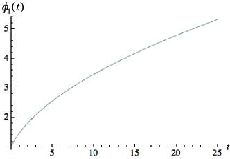
Figure 3: Plot of $\phi_{1}(t)$ in Eq. (51) which describes the contribution to the ground-state energy (50) from spin fluctuations due to the quadratic Zeeman effect, where $t=q/(n|c_{1}^{(1)}|)-1$.

The pressure and sound velocity are calculated as

$$P=\frac{n^{2}c_{0}^{(1)}}{2}\left(1+\frac{8\sqrt{M^{3}}}{5\pi^{2}\hbar^{3}}\sqrt{n(c_{0}^{(1)})^{3}}\right)+\frac{8\sqrt{M^{3}}n^{2}|c_{1}^{(1)}|}{15\pi^{2}\hbar^{3}}\sqrt{n(|c_{1}^{(1)}|)^{3}}\Big{[}3\phi_{1}(t_{1}+\text{sgn}(c_{1}^{(1)}))$$

$$-2(t_{1}+1)\phi^{\prime}_{1}(t_{1}+\text{sgn}(c_{1}^{(1)}))\Big{]},$$ (52)

and

$$c=\sqrt{\frac{nc_{0}^{(1)}}{M}}\Bigg{[}1+\frac{\sqrt{M^{3}}}{\pi^{2}\hbar^{3}}\sqrt{n(c_{0}^{(1)})^{3}}+\frac{2\sqrt{M^{3}}}{15\pi^{2}\hbar^{3}}\left(\frac{|c_{1}^{(1)}|}{c_{0}^{(1)}}\right)\sqrt{n(|c_{1}^{(1)}|)^{3}}\phi_{2}(t_{1},\text{sgn}(c_{1}^{(1)}))\Bigg{]},$$ (53)

where

$$\phi_{2}(t,\text{sgn}(c_{1}^{(1)}))\equiv 15\phi_{1}(t+\text{sgn}(c_{1}^{(1)}))-12(t+1)\phi^{\prime}_{1}(t+\text{sgn}(c_{1}^{(1)}))+4(t+1)^{2}\phi^{\prime\prime}_{1}(t+\text{sgn}(c_{1}^{(1)})),$$ (54)

which is plotted in Fig. 4. We note that for the case of $c_{1}^{(1)}<0$, the quantum correction to the sound velocity due to spin fluctuations vanishes at $t\simeq 1.4$.

Figure 4: Plot of $\phi_{2}(t,\text{sgn}(c_{1}^{(1)}))$ which gives the correction to the sound velocity (53) due to the quadratic Zeeman effect.

On the other hand, the quantum depletion is calculated to be

$$\frac{N-N_{0}}{N} = \frac{1}{N}{\sum_{\mathbf{k}}}^{{}^{\prime}}\langle\hat{a}^{\dagger}_{\mathbf{k},d}\hat{a}_{\mathbf{k},d}+\hat{a}^{\dagger}_{\mathbf{k},f_{x}}\hat{a}_{\mathbf{k},f_{x}}+\hat{a}^{\dagger}_{\mathbf{k},f_{y}}\hat{a}_{\mathbf{k},f_{y}}\rangle$$ (55)

$$= \frac{\sqrt{M^{3}}}{3\pi^{2}\hbar^{3}}\left(\sqrt{n(c_{0}^{(1)})^{3}}+2\sqrt{n(|c_{1}^{(1)}|)^{3}}\phi_{3}(t_{1}+\text{sgn}(c_{1}^{(1)}))\right),$$

where

$$\phi_{3}(t)\equiv\frac{3}{\sqrt{2}}\int_{0}^{\infty}dx\ x^{2}\left(\frac{x^{2}+t+1}{\sqrt{(x^{2}+t)(x^{2}+t+2)}}-1\right).$$ (56)

The plot of $\phi_{3}(t)$ is shown in Fig. 5, which shows that the quantum depletion is suppressed by the quadratic Zeeman effect.

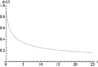
Figure 5: Plot of $\phi_{3}(t)$ which describes the quantum depletion through Eq. (55).

In contrast, the quantum corrections to the GSE and sound velocity are enhanced by it. Since the variations of $\phi_{1}(t)$, $\phi_{2}(t,\pm 1)$, and $\phi_{3}(t)$ in the typical region of $t$ are of the order of $1\sim 10$, the magnetic-field dependence of the LHY corrections is significant. However, because $c_{0}^{(1)}\gg c_{1}^{(1)}$ in the alkali species, the magnitudes of the LHY corrections are small and the quantum corrections arise mainly from density fluctuations.

IV.2.2 Case of $q<0$

To analyze the case of (24), we introduce the following fluctuation operators:

$$\hat{a}_{\mathbf{k},d}=\frac{1}{\sqrt{2}}(\hat{a}_{\mathbf{k},1}+\hat{a}_{\mathbf{k},-1}),$$ (57)

$$\hat{a}_{\mathbf{k},f_{x}}=\hat{a}_{\mathbf{k},0},$$ (58)

$$\hat{a}_{\mathbf{k},f_{z}}=\frac{1}{\sqrt{2}}(\hat{a}_{\mathbf{k},1}-\hat{a}_{\mathbf{k},-1}),$$ (59)

where $\hat{a}_{\mathbf{k},d}$, $\hat{a}_{\mathbf{k},f_{x}}$, and $\hat{a}_{\mathbf{k},f_{z}}$ describe the density fluctuation $(d)$ and spin fluctuations $(f_{x},f_{z})$ around the $x$ and $z$ axes, respectively. The Hamiltonian is diagonalized by the following Bogoliubov transformations

$$\hat{b}_{\mathbf{k},d}=\sqrt{\frac{\epsilon_{\mathbf{k}}+nc_{0}^{(1)}+E_{\mathbf{k},d}}{2E_{\mathbf{k},d}}}\hat{a}_{\mathbf{k},d}+\sqrt{\frac{\epsilon_{\mathbf{k}}+nc_{0}^{(1)}-E_{\mathbf{k},d}}{2E_{\mathbf{k},d}}}\hat{a}^{\dagger}_{\mathbf{-k},d},$$ (60)

$$\hat{b}_{\mathbf{k},f_{x}}=\sqrt{\frac{\epsilon_{\mathbf{k}}-q+nc_{1}^{(1)}+E_{\mathbf{k},f_{x}}}{2E_{\mathbf{k},f_{x}}}}\hat{a}_{\mathbf{k},f_{x}}+\sqrt{\frac{\epsilon_{\mathbf{k}}-q+nc_{1}^{(1)}-E_{\mathbf{k},f_{x}}}{2E_{\mathbf{k},f_{x}}}}\hat{a}^{\dagger}_{\mathbf{-k},f_{x}},$$ (61)

$$\hat{b}_{\mathbf{k},f_{z}}=\sqrt{\frac{\epsilon_{\mathbf{k}}+nc_{1}^{(1)}+E_{\mathbf{k},f_{z}}}{2E_{\mathbf{k},f_{z}}}}\hat{a}_{\mathbf{k},f_{z}}+\sqrt{\frac{\epsilon_{\mathbf{k}}+nc_{1}^{(1)}-E_{\mathbf{k},f_{z}}}{2E_{\mathbf{k},f_{z}}}}\hat{a}^{\dagger}_{\mathbf{-k},f_{z}},$$ (62)

with the result

$$\hat{H}_{\text{eff}}^{P^{\prime}}=E_{0}^{P^{\prime}}+{\sum_{\mathbf{k}}}^{{}^{\prime}}\big{(}E_{\mathbf{k},d}\hat{b}^{\dagger}_{\mathbf{k},d}\hat{b}_{\mathbf{k},d}+E_{\mathbf{k},f_{x}}\hat{b}^{\dagger}_{\mathbf{k},f_{x}}\hat{b}_{\mathbf{k},f_{x}}+E_{\mathbf{k},f_{z}}\hat{b}^{\dagger}_{\mathbf{k},f_{z}}\hat{b}_{\mathbf{k},f_{z}}\big{)},$$ (63)

where

$$E_{0}^{P^{\prime}}=qN+\frac{Vn^{2}\bar{c}_{0}^{(1)}}{2}-\frac{1}{2}{\sum_{\mathbf{k}}}^{{}^{\prime}}\Bigg{[}\left(\epsilon_{\mathbf{k}}+nc_{0}^{(1)}-E_{\mathbf{k},d}\right)+\left(\epsilon_{\mathbf{k}}-q+nc_{1}^{(1)}-E_{\mathbf{k},f_{x}}\right)$$

$$+\left(\epsilon_{\mathbf{k}}+nc_{1}^{(1)}-E_{\mathbf{k},f_{x}}\right)\Bigg{]}$$ (64)

is the GSE, and the Bogoliubov spectra are given by

$$E_{\mathbf{k},d}=\sqrt{\epsilon_{\mathbf{k}}\left(\epsilon_{\mathbf{k}}+2nc_{0}^{(1)}\right)},$$ (65)

$$E_{\mathbf{k},f_{x}}=\sqrt{(\epsilon_{\mathbf{k}}-q)\left(\epsilon_{\mathbf{k}}-q+2nc_{1}^{(1)}\right)},$$ (66)

$$E_{\mathbf{k},f_{z}}=\sqrt{\epsilon_{\mathbf{k}}\left(\epsilon_{\mathbf{k}}+2nc_{1}^{(1)}\right)}.$$ (67)

In contrast to the case of $q>0$, one of the spin fluctuation modes, (67), becomes massless. This is because all the continuous symmetries of the Hamiltonian are spontaneously broken for $q<0$. On the other hand, the transverse spin mode is massive because the rotational symmetry about the $x$ axis is broken by an external magnetic field. For the Bogoliubov spectra to be real, the conditions $q<0$, $c_{0}^{(1)}>0$, and $c_{1}^{(1)}>0$ must be satisfied; otherwise, the state in Eq. (24) would be dynamically unstable. The GSE $E_{0}^{P^{\prime}}$, pressure $P$, sound velocity $c$, and quantum depletion $(N-N_{0})/N$ are given by

$$\frac{E_{0}^{P^{\prime}}}{V}=qn+\frac{n^{2}c_{0}^{(1)}}{2}\left(1+\frac{16\sqrt{M^{3}}}{15\pi^{2}\hbar^{3}}\sqrt{n(c_{0}^{(1)})^{3}}\right)+\frac{8\sqrt{M^{3}}n^{2}c_{1}^{(1)}}{15\pi^{2}\hbar^{3}}\sqrt{n(c_{1}^{(1)})^{3}}(1+\phi_{1}(t_{2})),$$ (68)

$$P=\frac{n^{2}c_{0}^{(1)}}{2}\left(1+\frac{8\sqrt{M^{3}}}{5\pi^{2}\hbar^{3}}\sqrt{n(c_{0}^{(1)})^{3}}\right)+\frac{4\sqrt{M^{3}}n^{2}c_{1}^{(1)}}{15\pi^{2}\hbar^{3}}\sqrt{n(c_{1}^{(1)})^{3}}(3+3\phi_{1}(t_{2})-2t_{2}\phi^{\prime}_{1}(t_{2})),$$ (69)

$$c=\sqrt{\frac{nc_{0}^{(1)}}{M}}\Bigg{[}1+\frac{\sqrt{M^{3}}}{\pi^{2}\hbar^{3}}\sqrt{n(c_{0}^{(1)})^{3}}+\frac{\sqrt{M^{3}}}{15\pi^{2}\hbar^{3}}\left(\frac{c_{1}^{(1)}}{c_{0}^{(1)}}\right)\sqrt{n(c_{1}^{(1)})^{3}}(15+\phi_{2}(t_{2}-1,+1))\Bigg{]},$$ (70)

$$\frac{N-N_{0}}{N}=\frac{\sqrt{M^{3}}}{3\pi^{2}\hbar^{3}}\left(\sqrt{n(c_{0}^{(1)})^{3}}+\sqrt{n(c_{1}^{(1)})^{3}}(1+\phi_{3}(t_{2}))\right),$$ (71)

where $t_{2}=-q/(nc_{1}^{(1)})$. Reflecting the difference in the Bogoliubov spectra, the LHY corrections for Eq. (24) are also different from those for Eq. (23).

IV.3 Broken-axisymmetry phase

The mean-field ground state of the broken-axisymmetry phase is parametrized by Eq. (25). We define the following fluctuation operators:

$$\hat{a}_{\mathbf{k},d}=\frac{\sin\theta}{\sqrt{2}}\left(\hat{a}_{\mathbf{k},1}+\hat{a}_{\mathbf{k},-1}\right)+\cos\theta\hat{a}_{\mathbf{k},0},$$ (72)

$$\hat{a}_{\mathbf{k},f_{z}}=\frac{1}{\sqrt{2}}\left(\hat{a}_{\mathbf{k},1}-\hat{a}_{\mathbf{k},-1}\right).$$ (73)

In addition, we introduce the following operator that is independent of $\hat{a}_{\mathbf{k},d}$ and $\hat{a}_{\mathbf{k},f_{z}}$:

$$\hat{a}_{\mathbf{k},\theta}=\frac{\cos\theta}{\sqrt{2}}\left(\hat{a}_{\mathbf{k},1}+\hat{a}_{\mathbf{k},-1}\right)-\sin\theta\hat{a}_{\mathbf{k},0}.$$ (74)

In terms of them, the total Hamiltonian is expressed as

$$\hat{H}_{\text{eff}}^{BA} = \frac{Nq}{2}+\frac{Vn^{2}(\bar{c}_{0}^{(1)}+\bar{c}_{1}^{(1)})}{2}+\frac{Nq^{2}}{8n\bar{c}_{1}^{(1)}}+{\sum_{\mathbf{k}}}^{{}^{\prime}}\Bigg{[}\left(\epsilon_{\mathbf{k}}+\frac{q}{2}\right)\hat{a}^{\dagger}_{\mathbf{k},f_{z}}\hat{a}_{\mathbf{k},f_{z}}+\frac{q}{4}\left(\hat{a}_{\mathbf{k},f_{z}}\hat{a}_{\mathbf{-k},f_{z}}+\hat{a}^{\dagger}_{\mathbf{k},f_{z}}\hat{a}^{\dagger}_{\mathbf{-k},f_{z}}\right)$$ (75)

$$+\left(\epsilon_{\mathbf{k}}+nc_{0}^{(1)}+nc_{1}^{(1)}-nc_{q}^{(1)}\right)\hat{a}^{\dagger}_{\mathbf{k},d}\hat{a}_{\mathbf{k},d}+\left(\epsilon_{\mathbf{k}}-2nc_{1}^{(1)}+nc_{q}^{(1)}\right)\hat{a}^{\dagger}_{\mathbf{k},\theta}\hat{a}_{\mathbf{k},\theta}$$

$$+\frac{n(c_{0}^{(1)}+c_{1}^{(1)}-c_{q}^{(1)})}{2}\left(\hat{a}_{\mathbf{k},d}\hat{a}_{\mathbf{-k},d}+\hat{a}^{\dagger}_{\mathbf{k},d}\hat{a}^{\dagger}_{\mathbf{-k},d}\right)+\frac{nc_{q}^{(1)}}{2}\left(\hat{a}_{\mathbf{k},\theta}\hat{a}_{\mathbf{-k},\theta}+\hat{a}^{\dagger}_{\mathbf{k},\theta}\hat{a}^{\dagger}_{\mathbf{-k},\theta}\right)$$

$$-\frac{q\sin 2\theta}{2}\left(\hat{a}^{\dagger}_{\mathbf{k},d}\hat{a}_{\mathbf{k},\theta}+\hat{a}^{\dagger}_{\mathbf{k},\theta}\hat{a}_{\mathbf{k},d}+\hat{a}_{\mathbf{k},d}\hat{a}_{\mathbf{-k},\theta}+\hat{a}^{\dagger}_{\mathbf{k},d}\hat{a}^{\dagger}_{\mathbf{-k},\theta}\right)\Bigg{]},$$

where

$$c_{q}^{(1)}\equiv\frac{q^{2}}{4n^{2}c_{1}^{(1)}}.$$ (76)

To diagonalize the sub-Hamiltonian for the spin fluctuation mode around the $z$ axis, we perform the following transformation:

$$\hat{b}_{\mathbf{k},f_{z}}=\sqrt{\frac{\epsilon_{\mathbf{k}}+q/2+E_{\mathbf{k},f_{z}}}{2E_{\mathbf{k},f_{z}}}}\hat{a}_{\mathbf{k},f_{z}}+\sqrt{\frac{\epsilon_{\mathbf{k}}+q/2-E_{\mathbf{k},f_{z}}}{2E_{\mathbf{k},f_{z}}}}\hat{a}^{\dagger}_{\mathbf{-k},f_{z}},$$ (77)

where the Bogoliubov spectrum is given by

$$E_{\mathbf{k},f_{z}}=\sqrt{\epsilon_{\mathbf{k}}\left(\epsilon_{\mathbf{k}}+q\right)}.$$ (78)

On the other hand, for the density fluctuation mode and the $\theta$ mode in Eq. (74), we consider the following transformations:

$$\hat{\mathbf{B}}_{\mathbf{k}}=U(k)\hat{\mathbf{A}}_{\mathbf{k},d\theta}+V(k)\hat{\mathbf{A}^{\dagger}}_{\mathbf{-k},d\theta},$$ (79)

where the bold symbols represent the following set of the operators

$$\hat{\mathbf{B}}_{\mathbf{k}}=^{t}(\hat{b}_{\mathbf{k},-},\hat{b}_{\mathbf{k},+}),\ \ \hat{\mathbf{A}}_{\mathbf{k},d\theta}=^{t}(\hat{a}_{\mathbf{k},d},\hat{a}_{\mathbf{k},\theta}),$$ (80)

and $U(k)$ and $V(k)$ are $2\times 2$ real matrices,

$$U(k)=\frac{1}{2}\left(\begin{array}[]{cc}\frac{1}{2C_{1-}(k)E_{1}(k)}+C_{1-}(k)X_{1+}(k)&q\epsilon_{\mathbf{k}}C_{1-}(k)\sin 2\theta-\frac{X_{1-}(k)}{2q\epsilon_{\mathbf{k}}C_{1-}(k)E_{1}(k)\sin 2\theta}\\ -\frac{1}{2C_{1+}(k)E_{1}(k)}+C_{1+}(k)X_{1-}(k)&q\epsilon_{\mathbf{k}}C_{1+}(k)\sin 2\theta+\frac{X_{1+}(k)}{2q\epsilon_{\mathbf{k}}C_{1+}(k)E_{1}(k)\sin 2\theta}\end{array}\right),$$ (83)

$$V(k)=\frac{1}{2}\left(\begin{array}[]{cc}-\frac{1}{2C_{1-}(k)E_{1}(k)}+C_{1-}(k)X_{1+}(k)&q\epsilon_{\mathbf{k}}C_{1-}(k)\sin 2\theta+\frac{X_{1-}(k)}{2q\epsilon_{\mathbf{k}}C_{1-}(k)E_{1}(k)\sin 2\theta}\\ \frac{1}{2C_{1+}(k)E_{1}(k)}+C_{1+}(k)X_{1-}(k)&-q\epsilon_{\mathbf{k}}C_{1+}(k)\sin 2\theta-\frac{X_{1+}(k)}{2q\epsilon_{\mathbf{k}}C_{1+}(k)E_{1}(k)\sin 2\theta}\end{array}\right),$$ (86)

with

$$X_{1\pm}(k)=-n(c_{0}^{(1)}+3c_{1}^{(1)}-2c_{q}^{(1)})\epsilon_{\mathbf{k}}+2n^{2}c_{1}^{(1)}(c_{1}^{(1)}-c_{q}^{(1)})\pm E_{1}(k),$$ (87)

$$E_{1}(k)=\Bigg{\{}[(n^{2}(c_{0}^{(1)}+3c_{1}^{(1)})^{2}-4n^{2}c_{q}^{(1)}(c_{0}^{(1)}+2c_{1}^{(1)})]\epsilon_{\mathbf{k}}^{2}-4n^{3}c_{1}^{(1)}(c_{0}^{(1)}+3c_{1}^{(1)})(c_{1}^{(1)}-c_{q}^{(1)})\epsilon_{\mathbf{k}}$$

$$+[2n^{2}c_{1}^{(1)}(c_{1}^{(1)}-c_{q}^{(1)})]^{2}\Bigg{\}}^{1/2},$$ (88)

$$C_{1\pm}(k)=\sqrt{\frac{E_{\mathbf{k},\pm}}{X^{2}_{1\mp}(k)\epsilon_{\mathbf{k}}+q^{2}\epsilon_{\mathbf{k}}^{2}(\epsilon_{\mathbf{k}}-2nc_{1}^{(1)})\sin^{2}2\theta}}.$$ (89)

In Eq. (89), $E_{\mathbf{k},\pm}$ are the Bogoliubov spectra given by

$$E_{\mathbf{k},\pm} = \sqrt{\epsilon_{\mathbf{k}}^{2}+n(c_{0}^{(1)}-c_{1}^{(1)})\epsilon_{\mathbf{k}}+2n^{2}c_{1}^{(1)}(c_{1}^{(1)}-c_{q}^{(1)})\pm E_{1}(k)}.$$ (90)

Using the transformations (79), the total Hamiltonian is diagonalized as

$$\hat{H}_{\text{eff}}^{BA}=E_{0}^{BA}+{\sum_{\mathbf{k}}}^{{}^{\prime}}\Bigg{[}E_{\mathbf{k},f_{z}}\hat{b}^{\dagger}_{\mathbf{k},f_{z}}\hat{b}_{\mathbf{k},f_{z}}+E_{\mathbf{k},-}\hat{b}^{\dagger}_{\mathbf{k},-}\hat{b}_{\mathbf{k},-}+E_{\mathbf{k},+}\hat{b}^{\dagger}_{\mathbf{k},+}\hat{b}_{\mathbf{k},+}\Bigg{]},$$ (91)

where the GSE is given by

$$E_{0}^{BA}=\frac{Nq}{2}+\frac{Vn^{2}(\bar{c}_{0}^{(1)}+\bar{c}_{1}^{(1)})}{2}+\frac{Nq^{2}}{8n\bar{c}_{1}^{(1)}}-\frac{1}{2}{\sum_{\mathbf{k}}}^{{}^{\prime}}\Big{[}\left(\epsilon_{\mathbf{k}}+q/2-E_{\mathbf{k},f_{z}}\right)$$

$$+(2\epsilon_{\mathbf{k}}+nc_{0}^{(1)}-nc_{1}^{(1)}-E_{\mathbf{k},+}-E_{\mathbf{k},-})\Big{]}.$$ (92)

Since $E_{\mathbf{k},-}^{2}\simeq 2n(c_{0}^{(1)}+c_{1}^{(1)})\epsilon_{\mathbf{k}}$ in the long-wavelength limit, $E_{\mathbf{k},-}$ is linear and massless. Furthermore, the $f_{z}$ mode is also linear and massless for nonzero $q$. This is because the $U(1)\times SO(2)$ symmetry is completely broken in the broken-axisymmetry phase. The positivity of the density and spin modes is ensured if $q>0$, $c_{1}^{(1)}<0$, $c_{0}^{(1)}+c_{1}^{(1)}>0$, and $q<-2c_{1}^{(1)}n$. Even though each mode is still massless for $q=0$, in the long-wavelength limit, the spectrum of $f_{z}$ changes from linear with $q\neq 0$ to quadratic with $q=0$. The physical origin of this change is discussed in Sec. V. Using the renormalization procedure discussed in Appendix A, we find that the GSE per volume $V$ in the broken-axisymmetry phase is given by

$$\frac{E_{0}^{BA}}{V} = \frac{nq}{2}+\frac{n^{2}(c_{0}^{(1)}+c_{1}^{(1)})}{2}+\frac{q^{2}}{8c_{1}^{(1)}}+\frac{\sqrt{2M^{3}q^{5}}}{15\pi^{2}\hbar^{3}}+\frac{8\sqrt{M^{3}}[n(c_{0}^{(1)}+c_{1}^{(1)})]^{\frac{5}{2}}}{15\pi^{2}\hbar^{3}}\phi_{4}(t_{3}),$$ (93)

with $t_{3}=q^{2}/(nc_{0}^{(1)}+nc_{1}^{(1)})^{2}$. Here

$$\phi_{4}(t) \equiv -\frac{15}{8\sqrt{2}}\int_{0}^{\infty}dxx^{2}\left(2x^{2}+y_{1}-\phi_{4}^{(+)}(t)-\phi_{4}^{(-)}(t)-\frac{1}{2x^{2}}+\frac{c_{0}^{(1)}t}{4c_{1}^{(1)}x^{2}}\right),$$ (94)

$$\phi_{4}^{(\pm)}(t) \equiv \sqrt{x^{4}+y_{1}x^{2}+y_{2}(t)\pm\sqrt{y_{3}(t)x^{4}+y_{4}(t)x^{2}+y_{2}^{2}(t)}},$$ (95)

with $y_{1}=(c_{0}^{(1)}-c_{1}^{(1)})/(c_{0}^{(1)}+c_{1}^{(1)})$, $y_{2}(t)=(2c_{1}^{(1)})^{2}/(c_{0}^{(1)}+c_{1}^{(1)})^{2}-t/2$, $y_{3}(t)=(c_{0}^{(1)}+3c_{1}^{(1)})^{2}/(c_{0}^{(1)}+c_{1}^{(1)})^{2}-(c_{0}^{(1)}+2c_{1}^{(1)})t/c_{1}^{(1)}$, and $y_{4}(t)=-4(c_{1}^{(1)})^{2}(c_{0}^{(1)}+3c_{1}^{(1)})/(c_{0}^{(1)}+c_{1}^{(1)})^{3}+(c_{0}^{(1)}+3c_{1}^{(1)})t/(c_{0}^{(1)}+c_{1}^{(1)})$. The behavior of $\phi_{4}(t)$ is shown in Fig. 6, where the typical values of $t$ for ⁸⁷Rb is $10^{-5}$. As can be seen from Fig. 6(a), the density component of the GSE increases slightly due to the quadratic Zeeman effect.

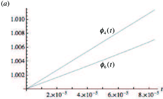
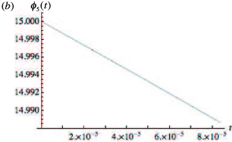
Figure 6: Plots of (a) $\phi_{4}(t)$ and $\phi_{6}(t)$, and (b) $\phi_{5}(t)$. Over the ranges of $t$ shown, they are well approximated as $\phi_{4}(t)\simeq 1+135t$ and $\phi_{6}(t)\simeq 1+80t+50000t^{2}$. ($\phi_{5}(t)$ is given by (98))

The pressure and the sound velocity are

$$P=\frac{n^{2}(c_{0}^{(1)}+c_{1}^{(1)})}{2}-\frac{q^{2}}{8c_{1}^{(1)}}-\frac{\sqrt{2M^{3}q^{5}}}{15\pi^{2}\hbar^{3}}+\frac{4\sqrt{M^{3}}[n(c_{0}^{(1)}+c_{1}^{(1)})]^{\frac{5}{2}}}{15\pi^{2}\hbar^{3}}(3\phi_{4}(t_{3})-4t_{3}\phi^{\prime}_{4}(t_{3})),$$ (96)

$$c=\sqrt{\frac{n(c_{0}^{(1)}+c_{1}^{(1)})}{M}}\left(1+\frac{\sqrt{M^{3}}}{15\pi^{2}\hbar^{3}}\sqrt{n(c_{0}^{(1)}+c_{1}^{(1)})^{3}}\phi_{5}(t_{3})\right),$$ (97)

where

$$\phi_{5}(t) \equiv 15\phi_{4}(t)-16t\phi^{\prime}_{4}(t)+16t^{2}\phi^{\prime\prime}_{4}(t).$$ (98)

The behavior of $\phi_{5}(t)$ in Fig. 6(b) shows that the LHY correction of the sound velocity decreases slightly as the external magnetic field increases.

The quantum depletion is

$$\frac{N-N_{0}}{N} = \frac{1}{N}{\sum_{\mathbf{k}}}^{{}^{\prime}}\langle\hat{a}^{\dagger}_{\mathbf{k},f_{z}}\hat{a}_{\mathbf{k},f_{z}}+\hat{a}^{\dagger}_{\mathbf{k},d}\hat{a}_{\mathbf{k},d}+\hat{a}^{\dagger}_{\mathbf{k},\theta}\hat{a}_{\mathbf{k},\theta}\rangle$$ (99)

$$= \frac{\sqrt{M^{3}}}{3\pi^{2}\hbar^{3}}\left(\sqrt{\frac{q^{3}}{8n^{2}}}+\sqrt{n(c_{0}^{(1)}+c_{1}^{(1)})^{3}}\phi_{6}(t_{3})\right),$$

with

$$\phi_{6}(t)\equiv\frac{6}{\sqrt{2}}\int_{0}^{\infty}dxx^{2}(V_{11}^{2}+V_{12}^{2}+V_{21}^{2}+V_{22}^{2}),$$ (100)

where $V_{ij}$’s are the the components of $V(k)$ in Eq. (86). The behavior of $\phi_{6}$ in Fig. 6(a) shows that the quantum depletion increases with increasing $t_{3}=q^{2}/(nc_{0}^{(1)}+nc_{1}^{(1)})^{2}$. However, the magnetic susceptibility of the quantum corrections in the broken-axisymmetry phase is small because the variations of $\phi_{4}(t)$, $\phi_{5}(t)$, and $\phi_{6}(t)$ over the typical range of $t$ are of the order of $10^{-2}$.

V Spin-2 BEC

For the case of a spin-2 BEC, the total spin in the two-body interaction $F$ takes on the values of 0, 2, or 4, and Eq. (7) reduces to ueda

$$\hat{H} = \sum_{\mathbf{k}}(\epsilon_{\mathbf{k}}+qm^{2})\hat{a}^{\dagger}_{\mathbf{k},m}\hat{a}_{\mathbf{k},m}+\frac{1}{2V}\sum_{\mathbf{k},\mathbf{p},\mathbf{q}}\Big{(}\bar{c}_{0}^{(2)}\hat{a}_{\mathbf{p},m}^{\dagger}\hat{a}_{\mathbf{q},m^{\prime}}^{\dagger}\hat{a}_{\mathbf{p+k},{m}}\hat{a}_{\mathbf{q-k},{m^{\prime}}}$$ (101)

$$+\bar{c}_{1}^{(2)}\mathbf{f}_{mm^{{}^{\prime}}}\cdot\mathbf{f}_{\mu\mu^{\prime}}\hat{a}_{\mathbf{p},m}^{\dagger}\hat{a}_{\mathbf{q},\mu}^{\dagger}\hat{a}_{\mathbf{p+k},{m^{{}^{\prime}}}}\hat{a}_{\mathbf{q-k},\mu^{\prime}}+\bar{c}_{2}^{(2)}(-1)^{m+m^{\prime}}\hat{a}_{\mathbf{p},m}^{\dagger}\hat{a}_{\mathbf{q},-m}^{\dagger}\hat{a}_{\mathbf{p+k},{m^{\prime}}}\hat{a}_{\mathbf{q-k},{-m^{\prime}}}\Big{)},$$

where $\bar{c}_{0}^{(2)}=(4\bar{g}_{2}+3\bar{g}_{4})/7,$ $\bar{c}_{1}^{(2)}=(\bar{g}_{4}-\bar{g}_{2})/7,$ $\bar{c}_{2}^{(2)}=(7\bar{g}_{0}-10\bar{g}_{2}+3\bar{g}_{4})/35,$ and the spin-2 matrices are given by

$${f}^{x} = \begin{pmatrix}0&1&0&0&0\\ 1&0&\sqrt{3\over 2}&0&0\\ 0&\sqrt{3\over 2}&0&\sqrt{3\over 2}&0\\ 0&0&\sqrt{3\over 2}&0&1\\ 0&0&0&1&0\end{pmatrix},\ \ \ {f}^{y}=\begin{pmatrix}0&-i&0&0&0\\ i&0&-i\sqrt{3\over 2}&0&0\\ 0&i\sqrt{3\over 2}&0&-i\sqrt{3\over 2}&0\\ 0&0&i\sqrt{3\over 2}&0&-i\\ 0&0&0&i&0\end{pmatrix},\ \ {f}^{z}=\begin{pmatrix}2&0&0&0&0\\ 0&1&0&0&0\\ 0&0&0&0&0\\ 0&0&0&-1&0\\ 0&0&0&0&-2\\ \end{pmatrix}.$$ (102)

The order parameter in a spin-2 BEC can be expanded in terms of the spherical harmonics of rank 2 as

$$\Psi=\sum_{m}\zeta_{m}\text{Y}^{m}_{2}(\mathbf{n})\equiv\frac{1}{2}\sqrt{\frac{15}{8\pi}}\mathbf{n}^{T}Q\mathbf{n},$$ (103)

where $\mathbf{n}=^{t}(n_{x},n_{y},n_{z})$ and

$$Q=\left(\begin{array}[]{ccc}\zeta_{2}+\zeta_{-2}-\sqrt{\frac{2}{3}}\zeta_{0}&i(\zeta_{2}-\zeta_{-2})&-\zeta_{1}+\zeta_{-1}\\ i(\zeta_{2}-\zeta_{-2})&-\zeta_{2}-\zeta_{-2}-\sqrt{\frac{2}{3}}\zeta_{0}&-i(\zeta_{1}+\zeta_{-1})\\ -\zeta_{1}+\zeta_{-1}&-i(\zeta_{1}+\zeta_{-1})&2\sqrt{\frac{2}{3}}\zeta_{0}\\ \end{array}\right)$$ (107)

is a traceless symmetric tensor mermin ; ueda . In the absence of an external magnetic field, the mean-field energy of a spin-2 BEC can be completely characterized by $Q$, and the ground-state phases are ferromagnetic, nematic, or cyclic, depending on the values of the coupling constants.

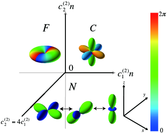
Figure 7: (Color online) Phase diagram of spin-2 BECs in the absence of an external magnetic field, where C, F, and N show the cyclic, ferromagnetic, and nematic phases, respectively. The thick lines represent the phase boundaries. The shape of the wave function is determined from $|\Psi(\theta,\phi)|^{2}\equiv|\sum_{m}\zeta_{m}\text{Y}_{2}^{m}(\theta,\phi)|^{2}$ and the color indicates the phase of $\Psi(\theta,\phi)$. The axes of the spin coordinate are depicted at the bottom right of the phase diagram. Note that the uniaxial (right) and biaxial (left) nematic phases are degenerate at the mean-field level.

The parameter regimes of these phases and the spinor order parameters are given by (see Fig. 7) ciobanu ; koashi ; ueda ; barnett ; mermin

$$\text{ferromagnetic phase:}\ \ \ c_{1}^{(2)}<0,\ \ c_{2}^{(2)}>4c_{1}^{(2)},\ \ \ \text{and}\ \ \ \mathbf{\zeta}^{F}=(1,0,0,0,0),$$ (108)

$$\text{nematic phase:}\ \ \ c_{2}^{(2)}<0,\ \ c_{2}^{(2)}<4c_{1}^{(2)},\ \text{and}\ \ \mathbf{\zeta}^{N}=\left(\frac{\sin\eta}{\sqrt{2}},0,\cos\eta,0,\frac{\sin\eta}{\sqrt{2}}\right),$$ (109)

$$\text{cyclic phase:}\ \ \ c_{1}^{(2)}>0,\ \ c_{2}^{(2)}>0,\ \text{and}\ \mathbf{\zeta}^{C}=\frac{1}{2}(1,0,\sqrt{2},0,-1),$$ (110)

where $c_{0}^{(2)}=(4g_{2}+3g_{4})/7$, $c_{1}^{(2)}=(g_{4}-g_{2})/7$, $c_{2}^{(2)}=(7g_{0}-10g_{2}+3g_{4})/35$. The nematic phase has no magnetization but features a finite spin-singlet pair amplitude, whereas the cyclic phase in the absence of an external magnetic field has neither magnetization nor spin-singlet amplitude. It is predicted ciobanu ; widera ; tojo that the ground states of ²³Na is nematic and that of ⁸⁷Rb lies in the vicinity of the phase boundary between the nematic and cyclic phases. (⁸⁵Rb is unstable at zero magnetic field in the thermodynamic limit because $c_{0}^{(2)}<0$.) The nematic phase has an additional continuous parameter $\eta$ (see $\zeta^{N}$ in Eq. (109)), which is not related to the symmetry of the Hamiltonian but represents the degeneracy of the uniaxial and biaxial spin nematic phases barnett ; turner ; song . However, this additional degeneracy arises only when the external magnetic field vanishes. In fact, for $q<0$, the biaxial nematic phase has a lower ground-state energy than the uniaxial nematic phase, and the boundaries and spinor order parameters are given as follows saito :

$$\text{ferromagnetic phase:}\ \ \ c_{2}^{(2)}>4c_{1}^{(2)},\ \ \ c_{1}^{(2)}<\frac{|q|}{2n},\ \ \ \text{and}\ \ \ \mathbf{\zeta}^{F}=(1,0,0,0,0),$$ (111)

$$\text{biaxial nematic phase:}\ \ \ c_{2}^{(2)}<4c_{1}^{(2)},\ \ c_{2}^{(2)}<\frac{2|q|}{n},\ \ \text{and}\ \ \mathbf{\zeta}^{BN}=\left(\frac{1}{\sqrt{2}},0,0,0,\frac{1}{\sqrt{2}}\right),$$ (112)

$$\text{cyclic phase:}\ \ \ c_{2}^{(2)}<4c_{1}^{(2)},\ \ c_{1}^{(2)}>\frac{|q|}{2n},\ \ c_{2}^{(2)}>\frac{2|q|}{n},\ \text{and}\ \mathbf{\zeta}^{C}=\left(\frac{\sin\theta}{\sqrt{2}},0,\cos\theta,0,-\frac{\sin\theta}{\sqrt{2}}\right),$$ (113)

$$\text{mixed phase:}\ \ \ c_{2}^{(2)}>4c_{1}^{(2)},\ \ c_{1}^{(2)}>\frac{|q|}{2n},\ \ c_{2}^{(2)}>\frac{2|q|}{n},\ \text{and}\ \mathbf{\zeta}^{M}=\left(\cos\theta^{\prime},0,0,\sin\theta^{\prime},0\right)\$$

$$\text{or}\ (0,\sin\theta^{\prime},0,0,\cos\theta^{\prime}),$$ (114)

where $\cos\theta=\sqrt{1/2+q/nc_{2}^{(2)}}$ and $\cos\theta^{\prime}=\sqrt{1/3-q/3nc_{1}^{(2)}}$. The phase diagram is shown in Fig. 8(a). The cyclic phase for $q<0$ does not have any magnetization but has a finite spin-singlet pair amplitude that depends on $q$. The mixed phase does not have a spin-singlet pair amplitude but has a finite longitudinal magnetization that depends on $q$.

On the other hand, for $q>0$, based on a numerical calculation, we find that the ground-state phases are given as follows:

$$\text{broken-axisymmetry phase:}\ \ \ \zeta^{BA}=(\pm a,b,c,b,\pm a),\ \ +\ (-)\ \text{sign for}\ c_{1}^{(2)}<0\ (>0)$$ (115)

$$\text{uniaxial nematic phase:}\ \ \ \zeta^{UN}=(0,0,1,0,0),$$ (116)

$$\text{cyclic phase:}\ \ \ \zeta^{C}=\left(\frac{\sin\theta}{\sqrt{2}},0,\cos\theta,0,-\frac{\sin\theta}{\sqrt{2}}\right),$$ (117)

where $a$, $b$, and $c$ are positive except for the case of $c_{1}^{(2)}=0$ and $c_{2}^{(2)}>0$, where $a=0$. The broken-axisymmetry phase has a transverse magnetization and a spin-singlet pair amplitude, both of which depend on $q$, as in the case of the spin-1 broken-axisymmetry phase. The phase boundaries between the broken-axisymmetry and cyclic phases and those between the cyclic and uniaxial nematic phases correspond to those between the mixed and cyclic phases and between the cyclic and biaxial nematic phases, respectively. The boundary between the broken-axisymmetry and uniaxial nematic phases is determined numerically. The phase diagram is shown in Fig. 8(b).

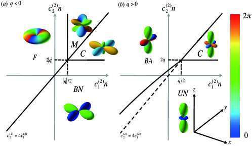
Figure 8: (Color online) Phase diagrams of spin-2 BECs for nonzero $q$. (a) Case of $q<0$, where BN, C, F, and M stand for the biaxial nematic, cyclic, ferromagnetic, and mixed phases, respectively. In the absence of an external magnetic field ($q=0$), the C and M states can be transformed to each other by a rotation in space. (b) Case of $q>0$, where the UN and BA stand for the uniaxial nematic and broken-axisymmetry phases, respectively. The thick lines show the phase boundaries.

The Bogoliubov Hamiltonian in a spin-2 BEC is given by ueda

$$\hat{H}_{\text{eff}} = \frac{Vn^{2}}{2}\left(\bar{c}_{0}^{(2)}+\bar{c}_{1}^{(2)}\langle\mathbf{f}\rangle^{2}+4\bar{c}_{2}^{(2)}|\langle s_{-}\rangle|^{2}\right)+qN\langle(f^{z})^{2}\rangle$$ (118)

$$+{\sum_{\mathbf{k}}}^{{}^{\prime}}\Bigg{[}\left(\epsilon_{\mathbf{k}}-nc_{1}^{(2)}\langle\mathbf{f}\rangle^{2}-4nc_{2}^{(2)}|\langle s_{-}\rangle|^{2}+qm^{2}-q\langle(f^{z})^{2}\rangle\right)\hat{a}^{\dagger}_{\mathbf{k},m}\hat{a}_{\mathbf{k},m}$$

$$+\frac{nc_{0}^{(2)}}{2}\left(2\hat{D}_{\mathbf{k}}^{\dagger}\hat{D}_{\mathbf{k}}+\hat{D}_{\mathbf{k}}\hat{D}_{\mathbf{-k}}+\hat{D}_{\mathbf{k}}^{\dagger}\hat{D}_{\mathbf{-k}}^{\dagger}\right)+\frac{nc_{1}^{(2)}}{2}\left(2\mathbf{\hat{F}}_{\mathbf{k}}^{\dagger}\cdot\mathbf{\hat{F}}_{\mathbf{k}}+\mathbf{\hat{F}}_{\mathbf{k}}\cdot\mathbf{\hat{F}}_{\mathbf{-k}}+\mathbf{\hat{F}}_{\mathbf{k}}^{\dagger}\cdot\mathbf{\hat{F}}_{\mathbf{-k}}^{\dagger}\right)$$

$$+nc_{1}^{(2)}\langle\mathbf{f}\rangle\cdot\mathbf{f}_{mm^{\prime}}\hat{a}^{\dagger}_{\mathbf{k},m}\hat{a}_{\mathbf{k},m^{\prime}}+2nc_{2}^{(2)}(\hat{S}^{-}_{\mathbf{k}})^{\dagger}\hat{S}^{-}_{\mathbf{k}}$$

$$+nc_{2}^{(2)}(-1)^{m}\left(\langle s_{-}\rangle\hat{a}^{\dagger}_{\mathbf{k},m}\hat{a}_{\mathbf{-k},-m}^{\dagger}+\langle s_{-}\rangle^{*}\hat{a}_{\mathbf{k},m}\hat{a}_{\mathbf{-k},-m}\right)\Bigg{]},$$

where

$$\langle s_{-}\rangle=\frac{1}{2}\sum_{m}(-1)^{m}\zeta_{m}\zeta_{-m}$$ (119)

is the spin-singlet pair amplitude, and

$$\hat{S}^{-}_{\mathbf{k}}=\sum_{m}(-1)^{m}\zeta_{m}\hat{a}_{\mathbf{k},-m},$$ (120)

is the pair fluctuation operator of the condensate. As in the case of a spin-1 BEC, we substitute $c_{i}^{(2)}$ for $\bar{c}_{i}^{(2)}$ $(i=0,1,2)$ in the sum over the momentum in Eq. (118).

V.1 Ferromagnetic phase

For the ferromagnetic phase (108), the sub-Hamiltonian with respect to $\hat{a}_{\mathbf{k},2}$ is diagonalized by the Bogoliubov transformation ueda

$$\hat{b}_{\mathbf{k},2}=\sqrt{\frac{\epsilon_{\mathbf{k}}+n(c_{0}^{(2)}+4c_{1}^{(2)})+E_{\mathbf{k},2}}{2E_{\mathbf{k},2}}}\hat{a}_{\mathbf{k},2}+\sqrt{\frac{\epsilon_{\mathbf{k}}+n(c_{0}^{(2)}+4c_{1}^{(2)})-E_{\mathbf{k},2}}{2E_{\mathbf{k},2}}}\hat{a}^{\dagger}_{\mathbf{-k},2},$$ (121)

with the Bogoliubov spectrum

$$E_{\mathbf{k},2}=\sqrt{\epsilon_{\mathbf{k}}\left[\epsilon_{\mathbf{k}}+2n(c_{0}^{(2)}+4c_{1}^{(2)})\right]}.$$ (122)

The diagonalized Hamiltonian is given by

$$\hat{H}_{\text{eff}}^{F} = E_{0}^{F}+{\sum_{\mathbf{k}}}^{{}^{\prime}}\Bigg{[}E_{\mathbf{k},2}\hat{b}^{\dagger}_{\mathbf{k},2}\hat{b}_{\mathbf{k},2}+(\epsilon_{\mathbf{k}}-3q)\hat{a}^{\dagger}_{\mathbf{k},1}\hat{a}_{\mathbf{k},1}+\left(\epsilon_{\mathbf{k}}-4q-4nc_{1}^{(2)}\right)\hat{a}^{\dagger}_{\mathbf{k},0}\hat{a}_{\mathbf{k},0}$$ (123)

$$+\left(\epsilon_{\mathbf{k}}-3q-6nc_{1}^{(2)}\right)\hat{a}^{\dagger}_{\mathbf{k},-1}\hat{a}_{\mathbf{k},-1}+\left(\epsilon_{\mathbf{k}}-8nc_{1}^{(2)}+2nc_{2}^{(2)}\right)\hat{a}^{\dagger}_{\mathbf{k},-2}\hat{a}_{\mathbf{k},-2}\Bigg{]},$$

where

$$E_{0}^{F}=4qN+\frac{Vn^{2}(\bar{c}_{0}^{(2)}+4\bar{c}_{1}^{(2)})}{2}-\frac{1}{2}{\sum_{\mathbf{k}}}^{{}^{\prime}}\left(\epsilon_{\mathbf{k}}+n(c_{0}^{(2)}+4c_{1}^{(2)})-E_{\mathbf{k},2}\right)$$ (124)

is the GSE. The $m=2$ mode is massless, and in the absence of an external magnetic field, the $m=1$ mode also becomes massless. For the excitation energies to be positive, we must have $c_{0}^{(2)}+4c_{1}^{(2)}>0$, $q<0$, $c_{1}^{(2)}<|q|/(2n)$, and $c_{2}^{(2)}>4c_{1}^{(2)}$. The GSE $E_{0}^{F}$, pressure $P$, sound velocity $c$, and quantum depletion $(N-N_{0})/N$ can be calculated as

$$\frac{E_{0}^{F}}{V}=4qn+\frac{2\pi\hbar^{2}n^{2}a_{4}}{M}\left(1+\frac{128}{15}\sqrt{\frac{na_{4}^{3}}{\pi}}\right),$$ (125)

$$P=\frac{2\pi\hbar^{2}n^{2}a_{4}}{M}\left(1+\frac{64}{5}\sqrt{\frac{na_{4}^{3}}{\pi}}\right),$$ (126)

$$c=\sqrt{\frac{4\pi\hbar^{2}na_{4}}{M^{2}}}\left(1+8\sqrt{\frac{na_{4}^{3}}{\pi}}\right),$$ (127)

$$\frac{N-N_{0}}{N}=\frac{8}{3}\sqrt{\frac{na_{4}^{3}}{\pi}},$$ (128)

where the renormalization of $\bar{g}_{4}$ is carried out to obtain the finite GSE.

V.2 Nematic phase

Let us next discuss the nematic phase. We discuss the cases of $q=0$ and $q\neq 0$ separately, since the stationary solutions are different.

V.2.1 Case of $q=0$

In the absence of an external magnetic field, the nematic phase is characterized by Eq. (109). We introduce the following four independent fluctuation operators:

$$\hat{a}_{\mathbf{k},d}=\frac{\sin\eta}{\sqrt{2}}(\hat{a}_{\mathbf{k},2}+\hat{a}_{\mathbf{k},-2})+\cos\eta\hat{a}_{\mathbf{k},0},$$ (129)

$$\hat{a}_{\mathbf{k},f_{x}}=\frac{1}{\sqrt{2}}(\hat{a}_{\mathbf{k},1}+\hat{a}_{\mathbf{k},-1}),$$ (130)

$$\hat{a}_{\mathbf{k},f_{y}}=\frac{i}{\sqrt{2}}(-\hat{a}_{\mathbf{k},1}+\hat{a}_{\mathbf{k},-1}),$$ (131)

$$\hat{a}_{\mathbf{k},f_{z}}=\frac{1}{\sqrt{2}}(\hat{a}_{\mathbf{k}2}-\hat{a}_{\mathbf{k},-2}),$$ (132)

where $\hat{a}_{\mathbf{k},d}$ and $\hat{a}_{\mathbf{k},f_{x,y,z}}$ describe density and spin fluctuations, respectively note:nematic . Furthermore, we introduce the following nematic fluctuation operator:

$$\hat{a}_{\mathbf{k},\eta}=\frac{\cos\eta}{\sqrt{2}}(\hat{a}_{\mathbf{k},2}+\hat{a}_{\mathbf{k},-2})-\sin\eta\hat{a}_{\mathbf{k},0}.$$ (133)

This operator describes fluctuations of the nematic order parameter; in fact, the coefficients in Eq. (133) are related to the nematic order parameter (109) by

$$\frac{\partial\mathbf{\zeta}^{N}}{\partial\eta}=\left(\frac{\cos\eta}{\sqrt{2}},0,-\sin\eta,0,\frac{\cos\eta}{\sqrt{2}}\right).$$ (134)

In terms of the operators in Eqs. (129)-(133), the total Hamiltonian can be decomposed into sub-Hamiltonians as

$$\hat{H}_{\text{eff}}^{N} = \frac{Vn^{2}(\bar{c}_{0}^{(2)}+\bar{c}_{2}^{(2)})}{2}+{\sum_{\mathbf{k}}}^{{}^{\prime}}\Bigg{\{}\left[\epsilon_{\mathbf{k}}+n(c_{0}^{(2)}+c_{2}^{(2)})\right]\hat{a}^{\dagger}_{\mathbf{k},d}\hat{a}_{\mathbf{k},d}+\frac{n(c_{0}^{(2)}+c_{2}^{(2)})}{2}(\hat{a}^{\dagger}_{\mathbf{k},d}\hat{a}^{\dagger}_{\mathbf{-k},d}+\hat{a}_{\mathbf{k},d}\hat{a}_{\mathbf{-k},d})$$ (135)

$$+\left[\epsilon_{\mathbf{k}}+nc_{3}^{(2)}(\eta+\pi/3)\right]\hat{a}^{\dagger}_{\mathbf{k},f_{x}}\hat{a}_{\mathbf{k},f_{x}}+\frac{nc_{3}^{(2)}(\eta+\pi/3)}{2}(\hat{a}^{\dagger}_{\mathbf{k},f_{x}}\hat{a}^{\dagger}_{\mathbf{-k},f_{x}}+\hat{a}_{\mathbf{k},f_{x}}\hat{a}_{\mathbf{-k},f_{x}})$$

$$+\left[\epsilon_{\mathbf{k}}+nc_{3}^{(2)}(\eta-\pi/3)\right]\hat{a}^{\dagger}_{\mathbf{k},f_{y}}\hat{a}_{\mathbf{k},f_{y}}-\frac{nc_{3}^{(2)}(\eta-\pi/3)}{2}(\hat{a}^{\dagger}_{\mathbf{k},f_{y}}\hat{a}^{\dagger}_{\mathbf{-k},f_{y}}+\hat{a}_{\mathbf{k},f_{y}}\hat{a}_{\mathbf{-k},f_{y}})$$

$$+\left[\epsilon_{\mathbf{k}}+nc_{3}^{(2)}(\eta)\right]\hat{a}^{\dagger}_{\mathbf{k},f_{z}}\hat{a}_{\mathbf{k},f_{z}}+\frac{nc_{3}^{(2)}(\eta)}{2}(\hat{a}^{\dagger}_{\mathbf{k},f_{z}}\hat{a}^{\dagger}_{\mathbf{-k},f_{z}}+\hat{a}_{\mathbf{k},f_{z}}\hat{a}_{\mathbf{-k},f_{z}})$$

$$+\left(\epsilon_{\mathbf{k}}-nc_{2}^{(2)}\right)\hat{a}^{\dagger}_{\mathbf{k},\eta}\hat{a}_{\mathbf{k},\eta}+\frac{nc_{2}^{(2)}}{2}(\hat{a}^{\dagger}_{\mathbf{k},\eta}\hat{a}^{\dagger}_{\mathbf{-k},\eta}+\hat{a}_{\mathbf{k},\eta}\hat{a}_{\mathbf{-k},\eta})\Bigg{\}},$$

where $\displaystyle c_{3}^{(2)}(\eta)\equiv 4c_{1}^{(2)}\sin^{2}\eta-c_{2}^{(2)}$. To diagonalize this Hamiltonian, we consider the following Bogoliubov transformations:

$$\hat{b}_{\mathbf{k},d}=\sqrt{\frac{\epsilon_{\mathbf{k}}+n(c_{0}^{(2)}+c_{2}^{(2)})+E_{\mathbf{k},d}}{E_{\mathbf{k},d}}}\hat{a}_{\mathbf{k},d}+\sqrt{\frac{\epsilon_{\mathbf{k}}+n(c_{0}^{(2)}+c_{2}^{(2)})-E_{\mathbf{k},d}}{E_{\mathbf{k},d}}}\hat{a}^{\dagger}_{\mathbf{-k},d},$$ (136)

$$\hat{b}_{\mathbf{k},f_{x}}=\sqrt{\frac{\epsilon_{\mathbf{k}}+nc_{3}^{(2)}(\eta+\pi/3)+E_{\mathbf{k},f_{x}}}{E_{\mathbf{k},f_{x}}}}\hat{a}_{\mathbf{k},f_{x}}+\sqrt{\frac{\epsilon_{\mathbf{k}}+nc_{3}^{(2)}(\eta+\pi/3)-E_{\mathbf{k},f_{x}}}{E_{\mathbf{k},f_{x}}}}\hat{a}^{\dagger}_{\mathbf{-k},f_{x}},$$ (137)

$$\hat{b}_{\mathbf{k},f_{y}}=\sqrt{\frac{\epsilon_{\mathbf{k}}+nc_{3}^{(2)}(\eta-\pi/3)+E_{\mathbf{k},f_{y}}}{E_{\mathbf{k},f_{y}}}}\hat{a}_{\mathbf{k},f_{y}}-\sqrt{\frac{\epsilon_{\mathbf{k}}+nc_{3}^{(2)}(\eta-\pi/3)-E_{\mathbf{k},f_{y}}}{E_{\mathbf{k},f_{y}}}}\hat{a}^{\dagger}_{\mathbf{-k},f_{y}},$$ (138)

$$\hat{b}_{\mathbf{k},f_{z}}=\sqrt{\frac{\epsilon_{\mathbf{k}}+nc_{3}^{(2)}(\eta)+E_{\mathbf{k},f_{z}}}{E_{\mathbf{k},f_{z}}}}\hat{a}_{\mathbf{k},f_{z}}+\sqrt{\frac{\epsilon_{\mathbf{k}}+nc_{3}^{(2)}(\eta)-E_{\mathbf{k},f_{z}}}{E_{\mathbf{k},f_{z}}}}\hat{a}^{\dagger}_{\mathbf{-k},f_{z}},$$ (139)

$$\hat{b}_{\mathbf{k},\eta}=\sqrt{\frac{\epsilon_{\mathbf{k}}-nc_{2}^{(2)}+E_{\mathbf{k},\eta}}{E_{\mathbf{k},\eta}}}\hat{a}_{\mathbf{k},\eta}-\sqrt{\frac{\epsilon_{\mathbf{k}}-nc_{2}^{(2)}-E_{\mathbf{k},\eta}}{E_{\mathbf{k},\eta}}}\hat{a}^{\dagger}_{\mathbf{-k},\eta},$$ (140)

where the Bogoliubov spectra are given byturner ; song

$$E_{\mathbf{k},d}=\sqrt{\epsilon_{\mathbf{k}}[\epsilon_{\mathbf{k}}+2n(c_{0}^{(2)}+c_{2}^{(2)})]},$$ (141)

$$E_{\mathbf{k},f_{x}}=\sqrt{\epsilon_{\mathbf{k}}[\epsilon_{\mathbf{k}}+2nc_{3}^{(2)}(\eta+\pi/3)]},$$ (142)

$$E_{\mathbf{k},f_{y}}=\sqrt{\epsilon_{\mathbf{k}}[\epsilon_{\mathbf{k}}+2nc_{3}^{(2)}(\eta-\pi/3)]},$$ (143)

$$E_{\mathbf{k},f_{z}}=\sqrt{\epsilon_{\mathbf{k}}[\epsilon_{\mathbf{k}}+2nc_{3}^{(2)}(\eta)]},$$ (144)

$$E_{\mathbf{k},\eta}=\sqrt{\epsilon_{\mathbf{k}}(\epsilon_{\mathbf{k}}-2nc_{2}^{(2)})}.$$ (145)

The diagonalized Hamiltonian is then given by

$$\hat{H}_{\text{eff}}^{N} = E_{0}^{N}(\eta)+{\sum_{\mathbf{k}}}^{{}^{\prime}}\Bigg{[}E_{\mathbf{k},d}\hat{b}^{\dagger}_{\mathbf{k},d}\hat{b}_{\mathbf{k},d}+E_{\mathbf{k},f_{x}}\hat{b}^{\dagger}_{\mathbf{k},f_{x}}\hat{b}_{\mathbf{k},f_{x}}+E_{\mathbf{k},f_{y}}\hat{b}^{\dagger}_{\mathbf{k},f_{y}}\hat{b}_{\mathbf{k},f_{y}}+E_{\mathbf{k},f_{z}}\hat{b}^{\dagger}_{\mathbf{k},f_{z}}\hat{b}_{\mathbf{k},f_{z}}+E_{\mathbf{k},\eta}\hat{b}^{\dagger}_{\mathbf{k},\eta}\hat{b}_{\mathbf{k},\eta}\Bigg{]},$$

where

$$E_{0}^{N}(\eta) = \frac{Vn^{2}(\bar{c}_{0}^{(2)}+\bar{c}_{2}^{(2)})}{2}-\frac{1}{2}{\sum_{\mathbf{k}}}^{{}^{\prime}}\Bigg{[}\left(\epsilon_{\mathbf{k}}+n(c_{0}^{(2)}+c_{2}^{(2)})-E_{\mathbf{k},d}\right)+\left(\epsilon_{\mathbf{k}}+nc_{3}^{(2)}(\eta+\pi/3)-E_{\mathbf{k},f_{x}}\right)$$

$$+\left(\epsilon_{\mathbf{k}}+nc_{3}^{(2)}(\eta-\pi/3)-E_{\mathbf{k},f_{y}}\right)+\left(\epsilon_{\mathbf{k}}+nc_{3}^{(2)}(\eta)-E_{\mathbf{k},f_{z}}\right)+\left(\epsilon_{\mathbf{k}}-nc_{2}^{(2)}-E_{\mathbf{k},\eta}\right)\Bigg{]}.$$

Although the total number of the symmetry generators of the Hamiltonian is $4$, the five Bogoliubov massless modes emerge. The physical origin of this result is discussed in Sec. V. We also note that regardless of the value of $\eta$, the above Bogoliubov spectra are real if $c_{0}^{(2)}+c_{2}^{(2)}>0$, $c_{2}^{(2)}<0$, and $c_{2}^{(2)}<4c_{1}^{(2)}$, in agreement with the stability criteria of the mean-field ground state. As shown in Appendix A, the GSE $E_{0}^{N}(\eta)$, pressure, sound velocity, quantum depletion are respectively given by

$$\frac{E_{0}^{N}(\eta)}{V} = \frac{n^{2}(c_{0}^{(2)}+c_{2}^{(2)})}{2}\left(1+\frac{16\sqrt{M^{3}}}{15\pi^{2}\hbar^{3}}\sqrt{n(c_{0}^{(2)}+c_{2}^{(2)})^{3}}\right)+\frac{8\sqrt{M^{3}}}{15\pi^{2}\hbar^{3}}\Bigg{\{}(n|c_{2}^{(2)}|)^{\frac{5}{2}}$$ (148)

$$+[n(2c_{1}^{(2)}-c_{2}^{(2)})]^{\frac{5}{2}}\sum_{j=0}^{2}[1+X\cos(2\eta+2\pi j/3)]^{\frac{5}{2}}\Bigg{\}},$$

$$P(\eta) = \frac{n^{2}(c_{0}^{(2)}+c_{2}^{(2)})}{2}\left(1+\frac{8\sqrt{M^{3}}}{5\pi^{2}\hbar^{3}}\sqrt{n(c_{0}^{(2)}+c_{2}^{(2)})^{3}}\right)+\frac{4\sqrt{M^{3}}}{5\pi^{2}\hbar^{3}}\Bigg{\{}(n|c_{2}^{(2)}|)^{\frac{5}{2}}$$ (149)

$$+[n(2c_{1}^{(2)}-c_{2}^{(2)})]^{\frac{5}{2}}\sum_{j=0}^{2}[1+X\cos(2\eta+2\pi j/3)]^{\frac{5}{2}}\Bigg{\}},$$

$$c(\eta) = \sqrt{\frac{n(c_{0}^{(2)}+c_{2}^{(2)})}{M}}\Bigg{\{}1+\frac{\sqrt{M^{3}}}{\pi^{2}\hbar^{3}}\Bigg{[}\sqrt{n(c_{0}^{(2)}+c_{2}^{(2)})^{3}}-\frac{\sqrt{n(-c_{2}^{(2)})^{5}}}{c_{0}^{(2)}+c_{2}^{(2)}}$$ (150)

$$+\frac{\sqrt{n(2c_{1}^{(2)}-c_{2}^{(2)})^{5}}}{c_{0}^{(2)}+c_{2}^{(2)}}\sum_{j=0}^{2}(1+X\cos(2\eta+2\pi j/3))^{\frac{5}{2}}\Bigg{]}\Bigg{\}},$$

$$\frac{N-N_{0}}{N}=\frac{\sqrt{M^{3}}}{3\pi^{2}\hbar^{3}}\Bigg{[}\sqrt{n(c_{0}^{(2)}+c_{2}^{(2)})^{3}}+\sqrt{n\left(c_{3}^{(2)}(\eta+\pi/3)\right)^{3}}+\sqrt{n\left(c_{3}^{(2)}(\eta-\pi/3)\right)^{3}}$$

$$+\sqrt{n\left(c_{3}^{(2)}\left(\eta\right)\right)^{3}}+\sqrt{n(|c_{2}^{(2)}|)^{3}}\Bigg{]},$$ (151)

where $X=-2c_{1}^{(2)}/(2c_{1}^{(2)}-c_{2}^{(2)})$ and $2c_{1}^{(2)}-c_{2}^{(2)}\geq 0$ in the nematic phase.

We note that the GSE satisfies the following symmetries:

$$E_{0}^{N}(\eta+\pi/3)=E_{0}^{N}(\eta)\ \ \text{and}\ \ E_{0}^{N}(-\eta)=E_{0}^{N}(\eta).$$ (152)

Therefore, other physical properties derived from it such as the pressure, sound velocity, and quantum depletion also satisfy similar relations: we may therefore restrict the domain of the definition of $\eta$ to $\displaystyle 0\leq\eta<\pi/3$ to find the ground state. We define the part of the GSE that depends on $\eta$ as

$$E/\omega=\sum_{j=0}^{2}[1+X\cos(2\eta+2\pi j/3)]^{\frac{5}{2}},$$ (153)

where $\omega=8\sqrt{M^{3}}V[n(2c_{1}^{(2)}-c_{2}^{(2)})]^{\frac{5}{2}}/(15\pi^{2}\hbar^{3}).$ Since $\eta=0\ \text{and}\ \pi/6$ satisfy $\partial E/\partial\eta=0$, these points are the candidates of the ground state.

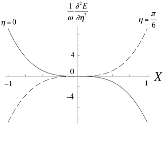
Figure 9: Second derivative of E with respect to $\eta$. The solid and dashed curves correspond to $\eta=0\ \text{and}\ \pi/6$, respectively.

The second derivative with respect to $\eta$ is plotted in FIG. 9, which shows that $\eta=0$ and $\eta=\pi/6$ correspond to the ground state for $X<0$ and $X>0$, respectively turner ; song . The phase transition between uniaxial and biaxial nematic phases occurs at $X=0$ because the diagonalized order-parameter matrices (107) for $X<0$ and $X>0$ given respectively by

$$Q_{X<0}=\left(\begin{array}[]{ccc}-\sqrt{\frac{2}{3}}&0&0\\ 0&-\sqrt{\frac{2}{3}}&0\\ 0&0&2\sqrt{\frac{2}{3}}\\ \end{array}\right)\ \ \text{and}\ \ Q_{X>0}=\left(\begin{array}[]{ccc}0&0&0\\ 0&-\sqrt{2}&0\\ 0&0&\sqrt{2}\\ \end{array}\right),$$ (160)

cannot be connected by any transformation that belongs to $U(1)\times SO(3)$ because Det$(Q_{X>0})=0$ and Det$(Q_{X<0})\neq 0$. The phase diagram that incorporates the quantum fluctuations arising from the Bogoliubov theory is depicted in Fig. 10. Here, we note that the many-body analysis in the single-mode approximation (SMA) koashi ; ueda ; uchino does not predict such a phase transition because the SMA ignores quantum fluctuations of momentum that play a crucial role in the phase transition between the uniaxial and biaxial nematic phases.

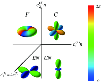
Figure 10: (Color online) Beyond-mean-field-theory phase diagram of spin-2 BECs in the absence of an external magnetic field obtained by the Bogoliubov theory, where C, F, UN, and BN stand for the cyclic, ferromagnetic, uniaxial nematic, and biaxial nematic phases, respectively. The thick lines show the phase boundaries. The phase diagram is consistent with that obtained in Refs. turner ; song .

We briefly comment on another stationary state $\displaystyle\zeta^{\prime}=\frac{1}{\sqrt{2}}(0,1,0,1,0)$. This state does not provide any new piece of information because it can be transformed into a biaxial nematic state by an element of $U(1)\times SO(3)$; in fact,

$$\zeta^{\prime}=e^{i\theta}e^{-i\gamma f^{z}}e^{-i\beta f^{y}}e^{-i\alpha f^{z}}\zeta^{BN},$$ (161)

where $\displaystyle\zeta^{BN}=\frac{1}{\sqrt{2}}(1,0,0,0,1)$, $\theta=\pi/2$, $\alpha=\pi/4$, $\beta=\pi/2$, and $\displaystyle\gamma=0$. Therefore, this state belongs to the biaxial nematic phase and it has the same spectra as the biaxial nematic state in the absence of an external magnetic field.

There is a hidden symmetry in the mean-field stationary solution of the nematic phase. The nematic phase is characterized as $|\langle s_{-}\rangle|=1/2$ and $\langle\mathbf{f}\rangle=\mathbf{0}$, both of which remain invariant under the $U(1)\times SO(3)$ transformations and are independent on $\eta$. In fact, we can show that the full symmetry group that leaves the nematic invariant is $U(1)\times SO(5)$, which includes the $U(1)\times SO(3)$ as a subgroup. This is confirmed by using the fact that the pair-singlet interaction term, which is proportional to $\bar{c}_{2}^{(2)}$ in the Hamiltonian, has the $SO(5)$ symmetry uchino , and that $\langle\mathbf{f}\rangle=\mathbf{0}$ if $|\langle s_{-}\rangle|=1/2$ ueda ; ciobanu . In Sec. VI, we discuss a role of the $SO(5)$ symmetry and relationship with the massless modes in the nematic phase.

V.2.2 Biaxial nematic phase

The effective Hamiltonian of the biaxial nematic phase defined in Eq. (112) can be decomposed by the transformations of Eqs. (129)- (133):

$$\hat{H}_{\text{eff}}^{BN} = \frac{Vn^{2}(\bar{c}_{0}^{(2)}+\bar{c}_{2}^{(2)})}{2}+4qN+{\sum_{\mathbf{k}}}^{{}^{\prime}}\Bigg{\{}(\epsilon_{\mathbf{k}}+nc_{0}^{(2)}+nc_{2}^{(2)})\hat{a}^{\dagger}_{\mathbf{k},d}\hat{a}_{\mathbf{k},d}$$ (162)

$$+\frac{n(c_{0}^{(2)}+c_{2}^{(2)})}{2}(\hat{a}_{\mathbf{k},d}\hat{a}_{\mathbf{-k},d}+\hat{a}^{\dagger}_{\mathbf{k},d}\hat{a}^{\dagger}_{\mathbf{-k},d})$$

$$+\sum_{j=f_{x},f_{y}}\Big{[}(\epsilon_{\mathbf{k}}-3q+nc_{1}^{(2)}-nc_{2}^{(2)})\hat{a}^{\dagger}_{\mathbf{k},j}\hat{a}_{\mathbf{k},j}+\frac{n(c_{1}^{(2)}-c_{2}^{(2)})}{2}(\hat{a}_{\mathbf{k},j}\hat{a}_{\mathbf{-k},j}+\hat{a}^{\dagger}_{\mathbf{k},j}\hat{a}^{\dagger}_{\mathbf{k},j})\Big{]}$$

$$+(\epsilon_{\mathbf{k}}+4nc_{1}^{(2)}-nc_{2}^{(2)})\hat{a}^{\dagger}_{\mathbf{k},f_{z}}\hat{a}_{\mathbf{k},f_{z}}+\frac{n(4c_{1}^{(2)}-c_{2}^{(2)})}{2}(\hat{a}_{\mathbf{k},f_{z}}\hat{a}_{\mathbf{-k},f_{z}}+\hat{a}^{\dagger}_{\mathbf{k},f_{z}}\hat{a}^{\dagger}_{\mathbf{-k},f_{z}})$$

$$+(\epsilon_{\mathbf{k}}-4q-nc_{2}^{(2)})\hat{a}^{\dagger}_{\mathbf{k},\eta}\hat{a}_{\mathbf{k},\eta}+\frac{nc_{2}^{(2)}}{2}(\hat{a}_{\mathbf{k},\eta}\hat{a}_{\mathbf{-k},\eta}+\hat{a}^{\dagger}_{\mathbf{k},\eta}\hat{a}^{\dagger}_{\mathbf{-k},\eta})\Bigg{\}}.$$

This Hamiltonian can be diagonalized by the following Bogoliubov transformations

$$\hat{b}_{\mathbf{k},d}=\sqrt{\frac{\epsilon_{\mathbf{k}}+n(c_{0}^{(2)}+c_{2}^{(2)})+E_{\mathbf{k},d}}{E_{\mathbf{k},d}}}\hat{a}_{\mathbf{k},d}+\sqrt{\frac{\epsilon_{\mathbf{k}}+n(c_{0}^{(2)}+c_{2}^{(2)})-E_{\mathbf{k},d}}{E_{\mathbf{k},d}}}\hat{a}^{\dagger}_{\mathbf{-k},d},$$ (163)

$$\hat{b}_{\mathbf{k},j}=\sqrt{\frac{\epsilon_{\mathbf{k}}-3q+n(c_{1}^{(2)}-c_{2}^{(2)})+E_{\mathbf{k},f_{t}}}{E_{\mathbf{k},f_{t}}}}\hat{a}_{\mathbf{k},j}+\sqrt{\frac{\epsilon_{\mathbf{k}}-3q+n(c_{1}^{(2)}-c_{2}^{(2)})-E_{\mathbf{k},f_{t}}}{E_{\mathbf{k},f_{t}}}}\hat{a}^{\dagger}_{\mathbf{-k},j},$$ (164)

$$\hat{b}_{\mathbf{k},f_{z}}=\sqrt{\frac{\epsilon_{\mathbf{k}}+n(4c_{1}^{(2)}-c_{2}^{(2)})+E_{\mathbf{k},f_{z}}}{E_{\mathbf{k},f_{z}}}}\hat{a}_{\mathbf{k},f_{z}}+\sqrt{\frac{\epsilon_{\mathbf{k}}+n(4c_{1}^{(2)}-c_{2}^{(2)})-E_{\mathbf{k},f_{z}}}{E_{\mathbf{k},f_{z}}}}\hat{a}^{\dagger}_{\mathbf{-k},f_{z}},$$ (165)

$$\hat{b}_{\mathbf{k},\eta}=\sqrt{\frac{\epsilon_{\mathbf{k}}-4q-nc_{2}^{(2)}+E_{\mathbf{k},\eta}}{E_{\mathbf{k},\eta}}}\hat{a}_{\mathbf{k},\eta}-\sqrt{\frac{\epsilon_{\mathbf{k}}-4q-nc_{2}^{(2)}-E_{\mathbf{k},\eta}}{E_{\mathbf{k},\eta}}}\hat{a}^{\dagger}_{\mathbf{-k},\eta},$$ (166)

with the result

$$\hat{H}_{\text{eff}}^{BN}=E_{0}^{BN}+{\sum_{\mathbf{k}}}^{{}^{\prime}}\big{[}E_{\mathbf{k},d}\hat{b}^{\dagger}_{\mathbf{k},d}\hat{b}_{\mathbf{k},d}+E_{\mathbf{k},f_{t}}(\hat{b}^{\dagger}_{\mathbf{k},f_{x}}\hat{b}_{\mathbf{k},f_{x}}+\hat{b}^{\dagger}_{\mathbf{k},f_{y}}\hat{b}_{\mathbf{k},f_{y}})+E_{\mathbf{k},f_{z}}\hat{b}^{\dagger}_{\mathbf{k},f_{z}}\hat{b}_{\mathbf{k},f_{z}}+E_{\mathbf{k},\eta}\hat{b}^{\dagger}_{\mathbf{k},\eta}\hat{b}_{\mathbf{k},\eta}\big{]},$$

where

$$E_{0}^{BN} = \frac{Vn^{2}(\bar{c}_{0}^{(2)}+\bar{c}_{2}^{(2)})}{2}+4qN-\frac{1}{2}{\sum_{\mathbf{k}}}^{{}^{\prime}}\Bigg{[}\left(\epsilon_{\mathbf{k}}+nc_{0}^{(2)}+nc_{2}^{(2)}-E_{\mathbf{k},d}\right)$$ (168)

$$+2\left(\epsilon_{\mathbf{k}}-3q+nc_{1}^{(2)}-nc_{2}^{(2)}-E_{\mathbf{k},f_{t}}\right)$$

$$+\left(\epsilon_{\mathbf{k}}+4nc_{1}^{(2)}-nc_{2}^{(2)}-E_{\mathbf{k},f_{z}}\right)+\left(\epsilon_{\mathbf{k}}-4q-nc_{2}^{(2)}-E_{\mathbf{k},\eta}\right)\Bigg{]}$$

is the GSE, and the Bogoliubov spectra are given by

$$E_{\mathbf{k},d}=\sqrt{\epsilon_{\mathbf{k}}(\epsilon_{\mathbf{k}}+2n(c_{0}^{(2)}+c_{2}^{(2)}))},$$ (169)

$$E_{\mathbf{k},f_{t}}=\sqrt{(\epsilon_{\mathbf{k}}-3q)(\epsilon_{\mathbf{k}}-3q+2n(c_{1}^{(2)}-c_{2}^{(2)}))},$$ (170)

$$E_{\mathbf{k},f_{z}}=\sqrt{\epsilon_{\mathbf{k}}(\epsilon_{\mathbf{k}}+2n(4c_{1}^{(2)}-c_{2}^{(2)}))},$$ (171)

$$E_{\mathbf{k},\eta}=\sqrt{(\epsilon_{\mathbf{k}}-4q)(\epsilon_{\mathbf{k}}-4q-2nc_{2}^{(2)})}.$$ (172)

The density and spin fluctuations around the $z$ axis are massless and those of nematic and spin fluctuations around the $x$ and $y$ axes are massive. This is because the symmetry of the Hamiltonian is reduced to $U(1)\times SO(2)$ due to the external magnetic field and the fact that the isotropy group of the biaxial nematic phase does not include any continuous group. The Bogoliubov spectra in Eqs. (170) and (172) are positive semidefinite if $q<0$, which is consistent with the stability criterion of the mean-field ground state.

The GSE $E_{0}^{BN}$, pressure, sound velocity, and quantum depletion up to the LHY corrections are given as follows:

$$\frac{E_{0}^{BN}}{V} = 4qn+\frac{n^{2}(c_{0}^{(2)}+c_{2}^{(2)})}{2}\left(1+\frac{16\sqrt{M^{3}}}{15\pi^{2}\hbar^{3}}\sqrt{n(c_{0}^{(2)}+c_{2}^{(2)})^{3}}\right)+\frac{8\sqrt{M^{3}}}{15\pi^{2}\hbar^{3}}\Big{\{}(n|c_{2}^{(2)}|)^{\frac{5}{2}}\phi_{1}(t_{5}-\text{sgn}(c_{2}^{(2)}))$$ (173)

$$+2(n|c_{1}^{(2)}-c_{2}^{(2)}|)^{\frac{5}{2}}\phi_{1}(t_{4}+\text{sgn}(c_{1}^{(2)}-c_{2}^{(2)}))+[n(4c_{1}^{(2)}-c_{2}^{(2)})]^{\frac{5}{2}}\Big{\}},$$

$$P = \frac{n^{2}(c_{0}^{(2)}+c_{2}^{(2)})}{2}\left(1+\frac{8\sqrt{M^{3}}}{5\pi^{2}\hbar^{3}}\sqrt{n(c_{0}^{(2)}+c_{2}^{(2)})^{3}}\right)$$ (174)

$$+\frac{4\sqrt{M^{3}}}{15\pi^{2}\hbar^{3}}\Big{\{}(n|c_{2}^{(2)}|)^{\frac{5}{2}}\Big{[}3\phi_{1}(t_{5}-\text{sgn}(c_{2}^{(2)}))-2(t_{5}+1)\phi^{\prime}_{1}(t_{5}-\text{sgn}(c_{2}^{(2)}))\Big{]}$$

$$+2(n|c_{1}^{(2)}-c_{2}^{(2)}|)^{\frac{5}{2}}\Big{[}3\phi_{1}(t_{4}+\text{sgn}(c_{1}^{(2)}-c_{2}^{(2)}))-2(t_{4}+1)\phi^{\prime}_{1}(t_{4}+\text{sgn}(c_{1}^{(2)}-c_{2}^{(2)})\Big{]}$$

$$+3[n(4c_{1}^{(2)}-c_{2}^{(2)})]^{\frac{5}{2}}\Big{\}},$$

$$c = \sqrt{\frac{n(c_{0}^{(2)}+c_{2}^{(2)})}{M}}\Bigg{\{}1+\frac{\sqrt{M^{3}}}{\pi^{2}\hbar^{3}}\sqrt{n(c_{0}^{(2)}+c_{2}^{(2)})^{3}}+\frac{\sqrt{M^{3}}}{15\pi^{2}\hbar^{3}}\frac{\sqrt{n|c_{2}^{(2)}|^{5}}}{c_{0}^{(2)}+c_{2}^{(2)}}\phi_{2}(t_{5},-\text{sgn}(c_{2}^{(2)}))$$ (175)

$$+\frac{2\sqrt{M^{3}}}{15\pi^{2}\hbar^{3}}\frac{\sqrt{n|c_{1}^{(2)}-c_{2}^{(2)}|^{5}}}{c_{0}^{(2)}+c_{2}^{(2)}}\phi_{2}(t_{4},\text{sgn}(c_{1}^{(2)}-c_{2}^{(2)}))+\frac{\sqrt{M^{3}}}{\pi^{2}\hbar^{3}}\frac{\sqrt{n|4c_{1}^{(2)}-c_{2}^{(2)}|^{5}}}{c_{0}^{(2)}+c_{2}^{(2)}}\Bigg{\}},$$

$$\frac{N-N_{0}}{N} = \frac{\sqrt{M^{3}}}{3\pi^{2}\hbar^{3}}\Big{[}\sqrt{n(c_{0}^{(2)}+c_{2}^{(2)})^{3}}+2\sqrt{n|c_{1}^{(2)}-c_{2}^{(2)}|^{3}}+\sqrt{n(|c_{2}^{(2)}|)^{3}}\phi_{3}(t_{5}-\text{sgn}(c_{2}^{(2)}))$$ (176)

$$+\phi_{3}(t_{4}+\text{sgn}(c_{1}^{(2)}-c_{2}^{(2)}))+\sqrt{n(4c_{1}^{(2)}-c_{2}^{(2)})^{3}}\Big{]},$$

where $\displaystyle t_{4}=-3q/(n|c_{1}^{(2)}-c_{2}^{(2)}|)-1$ and $\displaystyle t_{5}=-4q/(n|c_{2}^{(2)}|)-1$. For $q<0$, all the LHY corrections are positive definite, indicating the robustness of the biaxial nematic phase against the beyond-Bogoliubov effect.

V.2.3 Uniaxial nematic phase

The effective Hamiltonian of the uniaxial nematic state in Eq. (116) is obtained by using the canonical transformations of Eqs. (129)- (133) as

$$\hat{H}_{\text{eff}}^{UN} = \frac{Vn^{2}(\bar{c}_{0}^{(2)}+\bar{c}_{2}^{(2)})}{2}+{\sum_{\mathbf{k}}}^{{}^{\prime}}\Bigg{\{}(\epsilon_{\mathbf{k}}+nc_{0}^{(2)}+nc_{2}^{(2)})\hat{a}^{\dagger}_{\mathbf{k},d}\hat{a}_{\mathbf{k},d}+\frac{n(c_{0}^{(2)}+c_{2}^{(2)})}{2}(\hat{a}_{\mathbf{k},d}\hat{a}_{\mathbf{-k},d}+\hat{a}^{\dagger}_{\mathbf{k},d}\hat{a}^{\dagger}_{\mathbf{-k},d})$$ (177)

$$+\sum_{j=f_{x},f_{y}}\Big{[}(\epsilon_{\mathbf{k}}+q+3nc_{1}^{(2)}-nc_{2}^{(2)})\hat{a}^{\dagger}_{\mathbf{k},j}\hat{a}_{\mathbf{k},j}+\frac{n(3c_{1}^{(2)}-c_{2}^{(2)})}{2}(\hat{a}_{\mathbf{k},j}\hat{a}_{\mathbf{-k},j}+\hat{a}^{\dagger}_{\mathbf{k},j}\hat{a}^{\dagger}_{\mathbf{k},j})\Big{]}$$

$$+\sum_{l=f_{z},\eta}\Big{[}(\epsilon_{\mathbf{k}}+4q-nc_{2}^{(2)})\hat{a}^{\dagger}_{\mathbf{k},l}\hat{a}_{\mathbf{k},l}+\frac{nc_{2}^{(2)}}{2}(\hat{a}_{\mathbf{k},l}\hat{a}_{\mathbf{-k},l}+\hat{a}^{\dagger}_{\mathbf{k},l}\hat{a}^{\dagger}_{\mathbf{-k},l})\Big{]}\Bigg{\}}.$$

This can be diagonalized by means of the following Bogoliubov transformations,

$$\hat{b}_{\mathbf{k},d}=\sqrt{\frac{\epsilon_{\mathbf{k}}+n(c_{0}^{(2)}+c_{2}^{(2)})+E_{\mathbf{k},d}}{E_{\mathbf{k},d}}}\hat{a}_{\mathbf{k},d}+\sqrt{\frac{\epsilon_{\mathbf{k}}+n(c_{0}^{(2)}+c_{2}^{(2)})-E_{\mathbf{k},d}}{E_{\mathbf{k},d}}}\hat{a}^{\dagger}_{\mathbf{-k},d},$$ (178)

$$\hat{b}_{\mathbf{k},j}=\sqrt{\frac{\epsilon_{\mathbf{k}}+q+n(3c_{1}^{(2)}-c_{2}^{(2)})+E_{\mathbf{k},f_{t}}}{E_{\mathbf{k},f_{t}}}}\hat{a}_{\mathbf{k},j}+\sqrt{\frac{\epsilon_{\mathbf{k}}+q+n(3c_{1}^{(2)}-c_{2}^{(2)})-E_{\mathbf{k},f_{t}}}{E_{\mathbf{k},f_{t}}}}\hat{a}^{\dagger}_{\mathbf{-k},j},$$ (179)

$$\hat{b}_{\mathbf{k},l}=\sqrt{\frac{\epsilon_{\mathbf{k}}+4q-nc_{2}^{(2)}+E_{\mathbf{k},\eta}}{E_{\mathbf{k},\eta}}}\hat{a}_{\mathbf{k},l}-\sqrt{\frac{\epsilon_{\mathbf{k}}+4q-nc_{2}^{(2)}-E_{\mathbf{k},\eta}}{E_{\mathbf{k},\eta}}}\hat{a}^{\dagger}_{\mathbf{-k},l},$$ (180)

with the result

$$\hat{H}_{\text{eff}}^{UN}=E_{0}^{UN}+{\sum_{\mathbf{k}}}^{{}^{\prime}}\big{[}E_{\mathbf{k},d}\hat{b}^{\dagger}_{\mathbf{k},d}\hat{b}_{\mathbf{k},d}+E_{\mathbf{k},f_{t}}(\hat{b}^{\dagger}_{\mathbf{k},f_{x}}\hat{b}_{\mathbf{k},f_{x}}+\hat{b}^{\dagger}_{\mathbf{k},f_{y}}\hat{b}_{\mathbf{k},f_{y}})+E_{\mathbf{k},\eta}(\hat{b}^{\dagger}_{\mathbf{k},f_{z}}\hat{b}_{\mathbf{k},f_{z}}+\hat{b}^{\dagger}_{\mathbf{k},\eta}\hat{b}_{\mathbf{k},\eta})\big{]},$$

where

$$E_{0}^{UN} = \frac{Vn^{2}(\bar{c}_{0}^{(2)}+\bar{c}_{2}^{(2)})}{2}-\frac{1}{2}{\sum_{\mathbf{k}}}^{{}^{\prime}}\Bigg{[}\left(\epsilon_{\mathbf{k}}+nc_{0}^{(2)}+nc_{2}^{(2)}-E_{\mathbf{k},d}\right)$$ (182)

$$+2\left(\epsilon_{\mathbf{k}}+q+3nc_{0}^{(2)}-nc_{2}^{(2)}-E_{\mathbf{k},f_{t}}\right)+2\left(\epsilon_{\mathbf{k}}+4q-nc_{2}^{(2)}-E_{\mathbf{k},\eta}\right)\Bigg{]}$$

is the GSE, and the Bogoliubov spectra are given by

$$E_{\mathbf{k},d}=\sqrt{\epsilon_{\mathbf{k}}(\epsilon_{\mathbf{k}}+2n(c_{0}^{(2)}+c_{2}^{(2)}))},$$ (183)

$$E_{\mathbf{k},f_{t}}=\sqrt{(\epsilon_{\mathbf{k}}+q)(\epsilon_{\mathbf{k}}+q+2n(3c_{1}^{(2)}-c_{2}^{(2)}))},$$ (184)

$$E_{\mathbf{k},\eta}=\sqrt{(\epsilon_{\mathbf{k}}+4q)(\epsilon_{\mathbf{k}}+4q-2nc_{2}^{(2)})}.$$ (185)

The density fluctuation is massless, while the nematic and spin fluctuations around all the axes are massive. This is because the isotropy group of the uniaxial nematic phase includes the continuous group $SO(2)$ and, therefore, one massless mode should appear. As can be seen from Eqs. (184) and (185), the Bogoliubov spectra are positive definite only if $q>0$, which is consistent with the mean-field analysis.

The GSE $E_{0}^{UN}$, pressure, sound velocity, and quantum depletion are given by

$$\frac{E_{0}^{UN}}{V} = \frac{n^{2}(c_{0}^{(2)}+c_{2}^{(2)})}{2}\left(1+\frac{16\sqrt{M^{3}}}{15\pi^{2}\hbar^{3}}\sqrt{n(c_{0}^{(2)}+c_{2}^{(2)})^{3}}\right)+\frac{16\sqrt{M^{3}}}{15\pi^{2}\hbar^{3}}\Big{[}(n|c_{2}^{(2)}|)^{\frac{5}{2}}\phi_{1}(t_{7}-\text{sgn}(c_{2}^{(2)}))$$ (186)

$$+(n|3c_{1}^{(2)}-c_{2}^{(2)}|)^{\frac{5}{2}}\phi_{1}(t_{6}+\text{sgn}(3c_{1}^{(2)}-c_{2}^{(2)}))\Big{]},$$

$$P = \frac{n^{2}(c_{0}^{(2)}+c_{2}^{(2)})}{2}\left(1+\frac{8\sqrt{M^{3}}}{5\pi^{2}\hbar^{3}}\sqrt{n(c_{0}^{(2)}+c_{2}^{(2)})^{3}}\right)$$

$$+\frac{8\sqrt{M^{3}}}{15\pi^{2}\hbar^{3}}\Big{\{}(n|c_{2}^{(2)}|)^{\frac{5}{2}}\Big{[}3\phi_{1}(t_{7}-\text{sgn}(c_{2}^{(2)}))-2(t_{7}+1)\phi^{\prime}_{1}(t_{7}-\text{sgn}(c_{2}^{(2)}))\Big{]}$$

$$+(n|3c_{1}^{(2)}-c_{2}^{(2)}|)^{\frac{5}{2}}\Big{[}3\phi_{1}(t_{6}+\text{sgn}(3c_{1}^{(2)}-c_{2}^{(2)}))-2(t_{6}+1)\phi^{\prime}_{1}(t_{6}+\text{sgn}(3c_{1}^{(2)}-c_{2}^{(2)}))\Big{]}\Big{\}},$$

$$c = \sqrt{\frac{n(c_{0}^{(2)}+c_{2}^{(2)})}{M}}\Bigg{[}1+\frac{\sqrt{M^{3}}}{\pi^{2}\hbar^{3}}\sqrt{n(c_{0}^{(2)}+c_{2}^{(2)})^{3}}+\frac{2\sqrt{M^{3}}}{15\pi^{2}\hbar^{3}}\Bigg{(}\frac{\sqrt{n|c_{2}^{(2)}|^{5}}}{c_{0}^{(2)}+c_{2}^{(2)}}\phi_{2}(t_{7},-\text{sgn}(c_{2}^{(2)}))$$ (188)

$$+\frac{\sqrt{n|3c_{1}^{(2)}-c_{2}^{(2)}|^{5}}}{c_{0}^{(2)}+c_{2}^{(2)}}\phi_{2}(t_{6},\text{sgn}(3c_{1}^{(2)}-c_{2}^{(2)}))\Bigg{)}\Bigg{]},$$

$$\frac{N-N_{0}}{N}=\frac{\sqrt{M^{3}}}{3\pi^{2}\hbar^{3}}\Big{[}\sqrt{n(c_{0}^{(2)}+c_{2}^{(2)})^{3}}+2\sqrt{n(|c_{2}^{(2)}|)^{3}}\phi_{3}(t_{7}-\text{sgn}(c_{2}^{(2)}))$$

$$+2\sqrt{n(|3c_{1}^{(2)}-c_{2}^{(2)}|)^{3}}\phi_{3}(t_{6}+\text{sgn}(3c_{1}^{(2)}-c_{2}^{(2)}))\Big{]},$$ (189)

where $t_{6}=q/(n|3c_{1}^{(2)}-c_{2}^{(2)}|)-1$, $t_{7}=q/(n|c_{2}^{(2)}|)-1$. The LHY corrections become imaginary for $q<0$, which implies that the system undergoes the dynamical instability, and that the uniaxial nematic phase is only stable for $q>0$.

V.3 Cyclic phase

In addition to the stable configuration of Eq. (113), we also examine the tetrahedral configuration of Eq. (110), even though the latter configuration is not a stationary solution of the mean-field theory for nonzero $q$. This is because the tetrahedral configuration has attracted considerable attention, since it gives rise to nontrivial phenomena such as the non-Abelian vortices zhou ; makela ; kobayashi .

V.3.1 Stable configuration for nonzero $q$

For the stable cyclic phase in Eq. (113), we consider the following canonical transformations:

$$\hat{a}_{\mathbf{k},d} = \frac{\sin\theta}{\sqrt{2}}(\hat{a}_{\mathbf{k},2}-\hat{a}_{\mathbf{k},-2})+\cos\theta\hat{a}_{\mathbf{k},0},$$ (190)

$$\hat{a}_{\mathbf{k},f_{x}} = \frac{\sin\theta+\sqrt{3}\cos\theta}{\sqrt{2\sin^{2}\theta+6\cos^{2}\theta}}\hat{a}_{\mathbf{k},1}+\frac{-\sin\theta+\sqrt{3}\cos\theta}{\sqrt{2\sin^{2}\theta+6\cos^{2}\theta}}\hat{a}_{\mathbf{k},-1},$$ (191)

$$\hat{a}_{\mathbf{k},f_{y}} = i\frac{-\sin\theta+\sqrt{3}\cos\theta}{\sqrt{2\sin^{2}\theta+6\cos^{2}\theta}}\hat{a}_{\mathbf{k},1}-i\frac{\sin\theta+\sqrt{3}\cos\theta}{\sqrt{2\sin^{2}\theta+6\cos^{2}\theta}}\hat{a}_{\mathbf{k},-1},$$ (192)

$$\hat{a}_{\mathbf{k},f_{z}} = \frac{1}{\sqrt{2}}(\hat{a}_{\mathbf{k},2}+\hat{a}_{\mathbf{k},-2}),$$ (193)

$$\hat{a}_{\mathbf{k},\theta} = \frac{\cos\theta}{\sqrt{2}}(-\hat{a}_{\mathbf{k},2}+\hat{a}_{\mathbf{k},-2})-\cos\theta\hat{a}_{\mathbf{k},0},$$ (194)

where $\hat{a}_{\mathbf{k},d}$, $\hat{a}_{\mathbf{k},f_{x}}$, $\hat{a}_{\mathbf{k},f_{y}}$, and $\hat{a}_{\mathbf{k},f_{z}}$ represent the density and spin fluctuations, and $\hat{a}_{\mathbf{k},\theta}$ is the operator that commute with the other four operators. Then, the Hamiltonian is given by

$$\hat{H}_{\text{eff}}^{C} = 2qN+\frac{Vn^{2}\bar{c}_{0}^{(2)}}{2}-\frac{2Vq^{2}}{\bar{c}_{2}^{(2)}}+{\sum_{\mathbf{k}}}^{{}^{\prime}}\Bigg{\{}\left[\epsilon_{\mathbf{k}}-q+2nc_{1}^{(2)}\left(1+\frac{q}{nc_{2}^{(2)}}\right)\right](\hat{a}^{\dagger}_{\mathbf{k},f_{x}}\hat{a}_{\mathbf{k},f_{x}}+\hat{a}^{\dagger}_{\mathbf{k},f_{y}}\hat{a}_{\mathbf{k},f_{y}})$$ (195)

$$+\left[nc_{1}^{(2)}\left(1+\frac{q}{nc_{2}^{(2)}}\right)-q\left(\frac{-\sin^{2}\theta+3\cos^{2}\theta}{\sin^{2}\theta+3\cos^{2}\theta}\right)\right]$$

$$\times(\hat{a}_{\mathbf{k},f_{x}}\hat{a}_{\mathbf{-k},f_{x}}+\hat{a}_{\mathbf{k},f_{y}}\hat{a}_{\mathbf{-k},f_{y}}+\hat{a}^{\dagger}_{\mathbf{k},f_{x}}\hat{a}^{\dagger}_{\mathbf{-k},f_{x}}+\hat{a}^{\dagger}_{\mathbf{k},f_{y}}\hat{a}^{\dagger}_{\mathbf{-k},f_{y}})$$

$$-\frac{2\sqrt{3}q\sin 2\theta}{\sin^{2}\theta+3\cos^{2}\theta}(\hat{a}_{\mathbf{k},f_{x}}\hat{a}_{\mathbf{-k},f_{y}}-\hat{a}^{\dagger}_{\mathbf{k},f_{x}}\hat{a}^{\dagger}_{\mathbf{-k},f_{y}})+\left(\epsilon_{\mathbf{k}}+2nc_{1}^{(2)}+2q-\frac{4qc_{1}^{(2)}}{c_{2}^{(2)}}\right)\hat{a}^{\dagger}_{\mathbf{k},f_{z}}\hat{a}_{\mathbf{k},f_{z}}$$

$$+\frac{1}{2}\left(2nc_{1}^{(2)}+2q-\frac{4qc_{1}^{(2)}}{c_{2}^{(2)}}\right)(\hat{a}_{\mathbf{k},f_{z}}\hat{a}_{\mathbf{-k},f_{z}}+\hat{a}^{\dagger}_{\mathbf{k},f_{z}}\hat{a}^{\dagger}_{\mathbf{-k},f_{z}})$$

$$+\left(\epsilon_{\mathbf{k}}+nc_{0}^{(2)}+nc_{q}^{(2)}\right)\hat{a}^{\dagger}_{\mathbf{k},d}\hat{a}_{\mathbf{k},d}+\frac{n(c_{0}^{(2)}+c_{q}^{(2)})}{2}(\hat{a}_{\mathbf{k},d}\hat{a}_{\mathbf{-k},d}+\hat{a}^{\dagger}_{\mathbf{k},d}\hat{a}^{\dagger}_{\mathbf{k},d})$$

$$+\left(\epsilon_{\mathbf{k}}+nc_{0}^{(2)}-nc_{q}^{(2)}\right)\hat{a}^{\dagger}_{\mathbf{k},\theta}\hat{a}_{\mathbf{k},\theta}-\frac{nc_{q}^{(2)}}{2}(\hat{a}_{\mathbf{k},\theta}\hat{a}_{\mathbf{-k},\theta}+\hat{a}^{\dagger}_{\mathbf{k},\theta}\hat{a}^{\dagger}_{\mathbf{k},\theta})$$

$$-2q\sin 2\theta(\hat{a}^{\dagger}_{\mathbf{k},d}\hat{a}_{\mathbf{k},\theta}+\hat{a}^{\dagger}_{\mathbf{k},\theta}\hat{a}_{\mathbf{k},\theta}+\hat{a}_{\mathbf{k},d}\hat{a}_{\mathbf{-k},\theta}+\hat{a}^{\dagger}_{\mathbf{k},d}\hat{a}^{\dagger}_{\mathbf{-k},\theta})\Bigg{\}},$$

where $c_{q}^{(2)}\equiv 4q^{2}/(n^{2}c_{2}^{(2)})$. For nonzero $q$, the above Hamiltonian is not decomposed into sub-Hamiltonians completely because all modes except for $\hat{a}_{\mathbf{k},f_{z}}$ couple. For the $f_{z}$ mode, we consider the following Bogoliubov transformation:

$$\hat{b}_{\mathbf{k},f_{z}}=\sqrt{\frac{\epsilon_{\mathbf{k}}+2nc_{1}^{(2)}+2q-4c_{1}^{(2)}q/c_{2}^{(2)}+E_{\mathbf{k},f_{z}}}{2E_{\mathbf{k},f_{z}}}}\hat{a}_{\mathbf{k},f_{z}}+\sqrt{\frac{\epsilon_{\mathbf{k}}+2nc_{1}^{(2)}+2q-4c_{1}^{(2)}q/c_{2}^{(2)}-E_{\mathbf{k},f_{z}}}{2E_{\mathbf{k},f_{z}}}}\hat{a}^{\dagger}_{\mathbf{-k},f_{z}},$$

where

$$E_{\mathbf{k},f_{z}}=\sqrt{\epsilon_{\mathbf{k}}\left(\epsilon_{\mathbf{k}}+4nc_{1}^{(2)}+4q-8c_{1}^{(2)}q/c_{2}^{(2)}\right)}$$ (197)

is the Bogoliubov spectrum. For the $f_{x}$ and $f_{y}$ modes, we consider the following Bogoliubov transformations:

$$\hat{b}_{\mathbf{k},f_{t1}} = \frac{1}{2}\Bigg{[}\sqrt{\frac{\epsilon_{\mathbf{k}}-q+2nc_{1}^{(2)}+2c_{1}^{(2)}q/c_{2}^{(2)}+E_{\mathbf{k},f_{t}}}{E_{\mathbf{k},f_{t}}}}(\hat{a}_{\mathbf{k},f_{x}}+\hat{a}_{\mathbf{k},f_{y}})$$ (198)

$$+e^{i\tau}\sqrt{\frac{\epsilon_{\mathbf{k}}-q+2nc_{1}^{(2)}+2c_{1}^{(2)}q/c_{2}^{(2)}-E_{\mathbf{k},f_{t}}}{E_{\mathbf{k},f_{t}}}}(\hat{a}^{\dagger}_{\mathbf{-k},f_{x}}+\hat{a}^{\dagger}_{\mathbf{-k},f_{y}})\Bigg{]},$$

$$\hat{b}_{\mathbf{k},f_{t2}} = \frac{1}{2}\Bigg{[}\sqrt{\frac{\epsilon_{\mathbf{k}}-q+2nc_{1}^{(2)}+2c_{1}^{(2)}q/c_{2}^{(2)}+E_{\mathbf{k},f_{t}}}{E_{\mathbf{k},f_{t}}}}(\hat{a}_{\mathbf{k},f_{x}}-\hat{a}_{\mathbf{k},f_{y}})$$ (199)

$$+e^{-i\tau}\sqrt{\frac{\epsilon_{\mathbf{k}}-q+2nc_{1}^{(2)}+2c_{1}^{(2)}q/c_{2}^{(2)}-E_{\mathbf{k},f_{t}}}{E_{\mathbf{k},f_{t}}}}(\hat{a}^{\dagger}_{\mathbf{-k},f_{x}}-\hat{a}^{\dagger}_{\mathbf{-k},f_{y}})\Bigg{]},$$

$$\beta=nc_{1}^{(2)}\left(1+\frac{q}{nc_{2}^{(2)}}\right)-q\left(\frac{-\sin^{2}\theta+3\cos^{2}\theta+2\sqrt{3}i\sin\theta\cos\theta}{\sin^{2}\theta+3\cos^{2}\theta}\right),$$ (200)

where $\tau\equiv-\text{Im}\beta/\text{Re}\beta$ and

$$E_{\mathbf{k},f_{t}}=\sqrt{3n^{2}c_{1}^{(2)}c_{q}^{(2)}-3q^{2}+\epsilon_{\mathbf{k}}\left(\epsilon_{\mathbf{k}}+4nc_{1}^{(2)}+4nc_{1}^{(2)}q/c_{2}^{(2)}-2q\right)},$$ (201)

is the doubly degenerate Bogoliubov spectrum. Finally, for the density and $\theta$ modes, we consider the following transformations:

$$\hat{\mathbf{B}}_{\mathbf{k}}=U(k)\hat{\mathbf{A}}_{\mathbf{k},d\theta}+V(k)\hat{\mathbf{A}^{\dagger}}_{\mathbf{-k},d\theta},$$ (202)

where $\hat{\mathbf{B}}_{\mathbf{k}}=^{t}(\hat{b}_{\mathbf{k},-},\hat{b}_{\mathbf{k},+}),\ \hat{\mathbf{A}}_{\mathbf{k},d\theta}=^{t}(\hat{a}_{\mathbf{k},d},\hat{a}_{\mathbf{k},\theta}),$

$$U(k)=\frac{1}{2}\left(\begin{array}[]{cc}\frac{1}{2C_{2-}(k)E_{2}(k)}+C_{2-}(k)X_{2+}(k)&4q\epsilon_{\mathbf{k}}C_{2-}(k)\sin 2\theta-\frac{X_{2-}(k)}{8q\epsilon_{\mathbf{k}}C_{2-}(k)E_{2}(k)\sin 2\theta}\\ -\frac{1}{2C_{2+}(k)E_{2}(k)}+C_{2+}(k)X_{2-}(k)&4q\epsilon_{\mathbf{k}}C_{2+}(k)\sin 2\theta+\frac{X_{2+}(k)}{8q\epsilon_{\mathbf{k}}C_{2+}(k)E_{2}(k)\sin 2\theta}\end{array}\right),$$ (205)

$$V(k)=\frac{1}{2}\left(\begin{array}[]{cc}-\frac{1}{2C_{2-}(k)E_{2}(k)}+C_{2-}(k)X_{2+}(k)&4q\epsilon_{\mathbf{k}}C_{2-}(k)\sin 2\theta+\frac{X_{2-}(k)}{8q\epsilon_{\mathbf{k}}C_{2-}(k)E_{2}(k)\sin 2\theta}\\ \frac{1}{2C_{2+}(k)E_{2}(k)}+C_{2+}(k)X_{2-}(k)&4q\epsilon_{\mathbf{k}}C_{2+}(k)\sin 2\theta-\frac{X_{2+}(k)}{8q\epsilon_{\mathbf{k}}C_{2+}(k)E_{2}(k)\sin 2\theta}\end{array}\right),$$ (208)

$$X_{2\pm}(k)=-n(c_{0}^{(2)}-2c_{2}^{(2)}+2c_{q}^{(2)})\epsilon_{\mathbf{k}}+2n^{2}c_{2}^{(2)}(c_{2}^{(2)}-c_{q}^{(2)})\pm E_{2}(k),$$ (209)

$$C_{2\pm}(k)=\sqrt{\frac{E_{\mathbf{k},\pm}}{X^{2}_{2\mp}(k)\epsilon_{\mathbf{k}}+16q^{2}\sin^{2}2\theta\epsilon_{\mathbf{k}}^{2}(\epsilon_{\mathbf{k}}+2nc_{2}^{(2)})}},$$ (210)

$$E_{2}(k)=\Bigg{\{}\{(nc_{0}^{(2)}-2nc_{2}^{(2)})^{2}+4n^{2}c_{q}^{(2)}(c_{0}^{(2)}-c_{2}^{(2)})\}\epsilon_{\mathbf{k}}^{2}-4n^{3}c_{2}^{(2)}(c_{0}^{(2)}-2c_{2}^{(2)})(c_{2}^{(2)}-c_{q}^{(2)})\epsilon_{\mathbf{k}}$$

$$+\{2n^{2}c_{2}^{(2)}(c_{2}^{(2)}-c_{q}^{(2)})\}^{2}\Bigg{\}}^{1/2},$$ (211)

and $E_{\mathbf{k},\pm}$ are the Bogoliubov spectra given by

$$E_{\mathbf{k},\pm}=\sqrt{\epsilon_{\mathbf{k}}\left(\epsilon_{\mathbf{k}}+nc_{0}^{(2)}+2nc_{2}^{(2)}\right)+2n^{2}c_{2}^{(2)}\left(c_{2}^{(2)}-c_{q}^{(2)}\right)\pm E_{2}(k)}.$$ (212)

Using the above transformations, the total Hamiltonian is diagonalized as follows:

$$\hat{H}_{\text{eff}}^{C}=E_{0}^{C}+{\sum_{\mathbf{k}}}^{{}^{\prime}}\Big{[}E_{\mathbf{k},f_{t}}(\hat{b}^{\dagger}_{\mathbf{k},f_{t1}}\hat{b}_{\mathbf{k},f_{t1}}+\hat{b}^{\dagger}_{\mathbf{k},f_{t2}}\hat{b}_{\mathbf{k},f_{t2}})+E_{\mathbf{k},f_{z}}\hat{b}^{\dagger}_{\mathbf{k},f_{z}}\hat{b}_{\mathbf{k},f_{z}}+E_{\mathbf{k},+}\hat{b}^{\dagger}_{\mathbf{k},+}\hat{b}_{\mathbf{k},+}+E_{\mathbf{k},-}\hat{b}^{\dagger}_{\mathbf{k},-}\hat{b}_{\mathbf{k},-}\Big{]},$$

where

$$E_{0}^{C} = 2qN+\frac{Vn^{2}\bar{c}_{0}^{(2)}}{2}-\frac{2Vq^{2}}{\bar{c}_{2}^{(2)}}-\frac{1}{2}{\sum_{\mathbf{k}}}^{{}^{\prime}}\Bigg{[}2\left(\epsilon_{\mathbf{k}}+2nc_{1}^{(2)}+2c_{1}^{(2)}q/c_{2}^{(2)}-q-E_{\mathbf{k},f_{t}}\right)$$

$$+\left(\epsilon_{\mathbf{k}}+2nc_{1}^{(2)}+2q-4c_{1}^{(2)}q/c_{2}^{(2)}-E_{\mathbf{k},f_{z}}\right)+\left(2\epsilon_{\mathbf{k}}+nc_{0}^{(2)}+2nc_{2}^{(2)}-E_{\mathbf{k},+}-E_{\mathbf{k},-}\right)\Bigg{]}.$$

In the long-wavelength limit, $E_{\mathbf{k},-}^{2}\simeq 2nc_{0}^{(2)}\epsilon_{\mathbf{k}}$; therefore, $E_{\mathbf{k},-}$ is linear and massless. This is the NG mode associated with the spontaneous breaking of the $U(1)$ gauge symmetry. The spectrum on the spin fluctuations around the $z$ axis is also linear and massless since the $SO(2)$ symmetry is spontaneously broken at the mean-field level. The spectra around the transverse axes are massive because the rotational symmetry about transverse directions are explicitly broken by an external magnetic field. We note that this cyclic configuration is stable if $c_{0}^{(2)}>c_{2}^{(2)}$, $c_{2}^{(2)}<4c_{1}^{(2)}$, $c_{1}^{(2)}>|q|/(2n)$, and $c_{2}^{(2)}>2|q|/n$. It is robust regardless the sign of $q$, which is consistent with the stability condition of the mean-field ground state. Using the renormalization procedure discussed in Appendix A, we find that the GSE per volume $V$ is given by

$$\frac{E_{0}^{C}}{V}=2qn+\frac{n^{2}c_{0}^{(2)}}{2}-\frac{2q^{2}}{c_{2}^{(2)}}+\frac{8\sqrt{M^{3}}}{15\pi^{2}\hbar^{3}}\Bigg{[}(2nc_{1}^{(2)}+2q-4c_{1}^{(2)}q/c_{2}^{(2)})^{\frac{5}{2}}+2(2nc_{1}^{(2)})^{\frac{5}{2}}\phi_{7\pm}(t_{8})$$

$$+(nc_{0}^{(2)})^{\frac{5}{2}}\phi_{8}(t_{9})\Bigg{]},$$ (215)

where the $+$ $(-)$ sign in $\phi_{7\pm}(t)$ corresponds to the case of $q>0$ $(q<0)$,

$$\phi_{7\pm}(t)\equiv-\frac{15}{8\sqrt{2}}\int_{0}^{\infty}dxx^{2}\left(x^{2}+z_{1\pm}(t)-\sqrt{z_{2}(t)+x^{2}(x^{2}+2z_{1\pm}(t))}-\frac{z_{1\pm}^{2}(t)-z_{2}(t)}{2x^{2}}\right),$$

$$\phi_{8}(t)\equiv-\frac{15}{8\sqrt{2}}\int_{0}^{\infty}dxx^{2}\left(2x^{2}+z_{3}-\phi_{8}^{(+)}(t)-\phi_{8}^{(-)}(t)-\frac{1}{2x^{2}}-\frac{z_{4}(t)}{x^{2}}\right),$$ (217)

$$\phi_{8}^{(\pm)}(t)\equiv\sqrt{x^{4}+z_{3}x^{2}+z_{5}(t)\pm\sqrt{z_{6}(t)x^{4}+z_{7}(t)x^{2}+z_{5}^{2}(t)}},$$ (218)

with $t_{8}=|q|/2nc_{1}^{(2)}$, $t_{9}=(2q)^{2}/(nc_{0}^{(2)})^{2}$, $z_{1\pm}(t)=1\mp t(1-2c_{1}^{(2)}/c_{2}^{(2)})$, $z_{2}(t)=t^{2}(12c_{1}^{(2)}/c_{2}^{(2)}-3)$, $z_{3}=(c_{0}^{(2)}+2c_{2}^{(2)})/c_{0}^{(2)}$, $z_{4}(t)=t(1+c_{0}^{(2)}/c_{2}^{(2)})$, $z_{5}(t)=2(c_{2}^{(2)}/c_{0}^{(2)})^{2}-2t$, $z_{6}(t)=(1-2c_{2}^{(2)}/c_{0}^{(2)})^{2}+4t(c_{0}^{(2)}/c_{2}^{(2)}-1)$, and $z_{7}(t)=-4(c_{2}^{(2)}/c_{0}^{(2)})(c_{0}^{(2)}-2c_{2}^{(2)})[c_{2}^{(2)}/(c_{0}^{(2)})^{2}-t/c_{2}^{(2)}]$. The plots of $\phi_{7\pm}(t)$ and $\phi_{8}(t)$ in Fig. 11 show that the spin components of the GSE around the $x$ and $y$ axes for $q<0$ (for $q>0$) decrease (increase), while the density component of the GSE increases as the external magnetic field increases. The typical values of $t_{8}$ and $t_{9}$ are of the order of $10^{-2}$ and $10^{-6}$, respectively, for the parameters of ⁸⁷Rb.

Figure 11: Plots of (a) $\phi_{7\pm}(t)$ and (b) $\phi_{8}(t)$. These functions are approximated as $\phi_{7\pm}(t)\simeq 1\pm 24.1t+116t^{2}$ and $\phi_{8}(t)\simeq 1+1140t$.

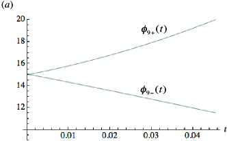
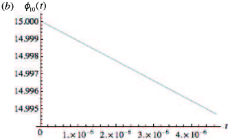
Figure 12: Plots of $\phi_{9\pm}(t)$ (a) and $\phi_{10}(t)$ (b).

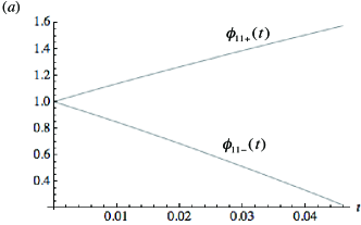
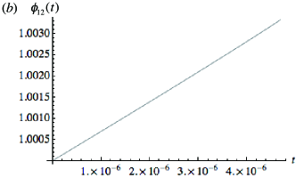
Figure 13: Plots of (a) $\phi_{11\pm}(t)$ and (b) $\phi_{12}(t)$. These functions are approximated as $\phi_{11-}(t)\simeq 1-15.1t-40t^{2}$, $\phi_{11+}(t)\simeq 1+13.6t-26t^{2}$, and $\phi_{12}(t)\simeq 1+700t$.

Performing the derivatives of the GSE with respect to $V$ and $n$, we obtain the pressure and sound velocity as follows:

$$P=\frac{n^{2}c_{0}^{(2)}}{2}+\frac{2q^{2}}{c_{2}^{(2)}}+\frac{4\sqrt{M^{3}}}{15\pi^{2}\hbar^{3}}\Bigg{[}(nc_{0}^{(2)})^{\frac{5}{2}}(3\phi_{8}(t_{9})-4t_{9}\phi_{8}^{\prime}(t_{9}))+(2nc_{1}^{(2)})^{\frac{5}{2}}(6\phi_{7\pm}(t_{8})-4t_{8}\phi_{7\pm}^{\prime}(t_{8}))$$

$$+\frac{3nc_{1}^{(2)}-2q+4c_{1}^{(2)}q/c_{2}^{(2)}}{nc_{1}^{(2)}+q-2c_{1}^{(2)}q/c_{2}^{(2)}}(2nc_{1}^{(2)}+2q-4c_{1}^{(2)}q/c_{2}^{(2)})^{\frac{5}{2}}\Bigg{]},$$

(219)

$$c = \sqrt{\frac{nc_{0}^{(2)}}{M}}\Bigg{[}1+\frac{\sqrt{M^{3}}}{15\pi^{2}\hbar^{3}}\sqrt{n(c_{0}^{(2)})^{3}}\phi_{10}(t_{9})+\frac{4\sqrt{M^{3}}}{15\pi^{2}\hbar^{3}}\frac{c_{1}^{(2)}}{c_{0}^{(2)}}\sqrt{n(2nc_{1}^{(2)})^{3}}\phi_{9\pm}(t_{8})$$ (220)

$$+\frac{4\sqrt{M^{3}}}{\pi^{2}\hbar^{3}}\frac{c_{1}^{(2)}}{c_{0}^{(2)}}\frac{nc_{1}^{(2)}}{2nc_{1}^{(2)}+2q-4c_{1}^{(2)}q/c_{2}^{(2)}}\sqrt{n\left(2c_{1}^{(2)}+2q/n-4c_{1}^{(2)}q/(nc_{2}^{(2)})\right)^{3}}\Bigg{]},$$

where

$$\phi_{9\pm}(t)\equiv 15\phi_{7\pm}(t)-12t\phi_{7\pm}^{\prime}(t)+4t^{2}\phi_{7\pm}^{\prime\prime}(t),$$ (221)

$$\phi_{10}(t)\equiv 15\phi_{8}(t)-16t\phi_{8}^{\prime}(t)+16t^{2}\phi_{8}^{\prime\prime}(t).$$ (222)

The behaviors of $\phi_{9\pm}(t)$ and $\phi_{10}(t)$ plotted in Fig. 12 show that for $q<0$ the sound velocities with respect to the density and spin wave around the $x$ and $y$ axes decrease, while for $q>0$ those with respect to the spin around the $x$ and $y$ axes increases, as the quadratic Zeeman effect becomes stronger. The quantum depletion is expressed as

$$\frac{N-N_{0}}{N}=\frac{\sqrt{M^{3}}}{3\pi^{2}\hbar^{3}}\Bigg{[}\sqrt{n\left(2q/n+2c_{1}^{(2)}-4c_{1}^{(2)}q/(nc_{2}^{(2)})\right)^{3}}+2\sqrt{n(2c_{1}^{(2)})^{3}}\phi_{11\pm}(t_{8})$$

$$+\sqrt{n(c_{0}^{(2)})^{3}}\phi_{12}(t_{9})\Bigg{]},$$ (223)

where the $+$ $(-)$ sign in $\phi_{11\pm}$ corresponds to the case of $q>0$ $(q<0)$, and

$$\phi_{11\pm}(t)\equiv\frac{3}{\sqrt{2}}\int dxx^{2}\left(\frac{x^{2}+1\mp t(1-2c_{1}^{(2)}/c_{2}^{(2)})}{\sqrt{3t^{2}(4c_{1}^{(2)}/c_{2}^{(2)}-1)+x^{2}(x^{2}+2\mp 2t(1-2c_{1}^{(2)}/c_{2}^{(2)}))}}-1\right),$$ (224)

$$\phi_{12}(t)\equiv\frac{6}{\sqrt{2}}\int_{0}^{\infty}dxx^{2}(V_{11}^{2}+V_{12}^{2}+V_{21}^{2}+V_{22}^{2}).$$ (225)

The behaviors of $\phi_{11\pm}(t)$ and $\phi_{12}(t)$ plotted in Fig. 13 show that the quantum depletion from the density fluctuations increases, while that from the spin fluctuations around the $x$ and $y$ axes for $q<0$ (for $q>0$) decreases (increases), as the external magnetic field increases. The variations of the quantum corrections with respect to the density component are small since the changes in $\phi_{8}(t)$, $\phi_{10}(t)$, and $\phi_{12}(t)$ are of the order of $10^{-3}$. On the other hand, the variations with respect to the spin components are of the order of 1. Considering the fact that $c_{0}^{(2)}\gg c_{1}^{(2)}$, $c_{2}^{(2)}$, and $|q|/n$ for the alkali species, however, the main contribution in the LHY corrections stems from the density fluctuations as in the cases of the other phases.

V.3.2 Tetrahedral configuration

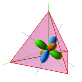
Figure 14: (Color online) Schematic illustration showing that the symmetry axes of the cyclic order parameter constitute a tetrahedron, where the color shows the phase of the order parameter as indicated in the color gauge of Fig. 7.

Finally, we examine the mean-field configuration of Eq. (110), which has the tetrahedral symmetry as shown in Fig. 14. We consider the following canonical transformations:

$$\hat{a}_{\mathbf{k},d} = \frac{1}{2}(\hat{a}_{\mathbf{k},2}-\hat{a}_{\mathbf{k},-2})+\frac{1}{\sqrt{2}}\hat{a}_{\mathbf{k},0},$$ (226)

$$\hat{a}_{\mathbf{k},f_{x}} = \frac{1+\sqrt{3}}{2\sqrt{2}}\hat{a}_{\mathbf{k},1}+\frac{-1+\sqrt{3}}{2\sqrt{2}}\hat{a}_{\mathbf{k},-1},$$ (227)

$$\hat{a}_{\mathbf{k},f_{y}} = i\frac{-1+\sqrt{3}}{2\sqrt{2}}\hat{a}_{\mathbf{k},1}-i\frac{1+\sqrt{3}}{2\sqrt{2}}\hat{a}_{\mathbf{k},-1},$$ (228)

$$\hat{a}_{\mathbf{k},f_{z}} = \frac{1}{\sqrt{2}}(\hat{a}_{\mathbf{k},2}+\hat{a}_{\mathbf{k},-2}),$$ (229)

$$\hat{a}_{\mathbf{k},p} = \frac{1}{2}(-\hat{a}_{\mathbf{k},2}+\hat{a}_{\mathbf{k},-2})+\frac{1}{\sqrt{2}}\hat{a}_{\mathbf{k},0},$$ (230)

which represent the density $(d)$, spin $(f_{x},f_{y},f_{z})$, and pair $(p)$ fluctuations, respectively. Then, the Hamiltonian is rewritten as follows:

$$\hat{H}_{\text{eff}}^{C} = 2qN+\frac{Vn^{2}\bar{c}_{0}^{(2)}}{2}+{\sum_{\mathbf{k}}}^{{}^{\prime}}\Bigg{\{}\sum_{j=f_{x},f_{y}}\Big{[}\left(\epsilon_{\mathbf{k}}-q+2nc_{1}^{(2)}\right)\hat{a}^{\dagger}_{\mathbf{k},j}\hat{a}_{\mathbf{k},j}+nc_{1}^{(2)}(\hat{a}_{\mathbf{k},j}\hat{a}_{\mathbf{-k},j}+\hat{a}^{\dagger}_{\mathbf{k},j}\hat{a}^{\dagger}_{\mathbf{-k},j})\Big{]}$$ (231)

$$+\left(\epsilon_{\mathbf{k}}+2q+2c_{1}^{(2)}\right)\hat{a}^{\dagger}_{\mathbf{k},f_{z}}\hat{a}_{\mathbf{k},f_{z}}+nc_{1}^{(2)}(\hat{a}^{\dagger}_{\mathbf{k},f_{z}}\hat{a}^{\dagger}_{\mathbf{-k},f_{z}}+\hat{a}_{\mathbf{k},f_{z}}\hat{a}_{\mathbf{-k},f_{z}})$$

$$+\left(\epsilon_{\mathbf{k}}+nc_{0}^{(2)}\right)\hat{a}^{\dagger}_{\mathbf{k},d}\hat{a}_{\mathbf{k},d}+\left(\epsilon_{\mathbf{k}}+2nc_{2}^{(2)}\right)\hat{a}^{\dagger}_{\mathbf{k},p}\hat{a}_{\mathbf{k},p}-2q(\hat{a}^{\dagger}_{\mathbf{k},d}\hat{a}_{\mathbf{k},p}+\hat{a}^{\dagger}_{\mathbf{k},p}\hat{a}_{\mathbf{k},d})$$

$$+\frac{nc_{0}^{(2)}}{2}(\hat{a}^{\dagger}_{\mathbf{k},d}\hat{a}^{\dagger}_{\mathbf{-k},d}+\hat{a}_{\mathbf{k},d}\hat{a}_{\mathbf{-k},d})\Bigg{\}}.$$

For nonzero $q$, the density fluctuation couples with the pair fluctuation. For the spin modes, we consider the following transformations:

$$\hat{b}_{\mathbf{k},j}=\sqrt{\frac{\epsilon_{\mathbf{k}}-q+2nc_{1}^{(2)}+E_{\mathbf{k},f_{t}}}{E_{\mathbf{k},f_{t}}}}\hat{a}_{\mathbf{k},j}+\sqrt{\frac{\epsilon_{\mathbf{k}}-q+2nc_{1}^{(2)}-E_{\mathbf{k},f_{t}}}{E_{\mathbf{k},f_{t}}}}\hat{a}^{\dagger}_{\mathbf{-k},j},$$ (232)

$$\hat{b}_{\mathbf{k},f_{z}}=\sqrt{\frac{\epsilon_{\mathbf{k}}+2q+2nc_{1}^{(2)}+E_{\mathbf{k},f_{z}}}{E_{\mathbf{k},f_{z}}}}\hat{a}_{\mathbf{k},f_{z}}+\sqrt{\frac{\epsilon_{\mathbf{k}}+2q+2nc_{1}^{(2)}-E_{\mathbf{k},f_{z}}}{E_{\mathbf{k},f_{z}}}}\hat{a}^{\dagger}_{\mathbf{-k},f_{z}},$$ (233)

where the Bogoliubov spectra are given by

$$E_{\mathbf{k},f_{t}}=\sqrt{(\epsilon_{\mathbf{k}}-q)\left(\epsilon_{\mathbf{k}}-q+4nc_{1}^{(2)}\right)},$$ (234)

$$E_{\mathbf{k},f_{z}}=\sqrt{(\epsilon_{\mathbf{k}}+2q)\left(\epsilon_{\mathbf{k}}+2q+4nc_{1}^{(2)}\right)}.$$ (235)

On the other hand, for the density and pair modes, we consider the following transformations:

$$\hat{\mathbf{B}}_{\mathbf{k}}=U(k)\hat{\mathbf{A}}_{\mathbf{k},dp}+V(k)\hat{\mathbf{A}^{\dagger}}_{\mathbf{-k},dp},$$ (236)

where $\hat{\mathbf{B}}_{\mathbf{k}}=^{t}(\hat{b}_{\mathbf{k},-},\hat{b}_{\mathbf{k},+}),\ \hat{\mathbf{A}}_{\mathbf{k},dp}=^{t}(\hat{a}_{\mathbf{k},d},\hat{a}_{\mathbf{k},p}),$

$$U(k)=\frac{1}{2}\left(\begin{array}[]{cc}\frac{1}{2C_{3-}(k)E_{3}(k)}+C_{3-}(k)X_{3+}(k)&4C_{3-}(k)q(\epsilon_{\mathbf{k}}+nc_{2}^{(2)})-\frac{X_{3-}(k)}{8C_{3-}(k)q(\epsilon_{\mathbf{k}}+nc_{2}^{(2)})E_{3}(k)}\\ -\frac{1}{2C_{3+}(k)E_{3}(k)}+C_{3+}(k)X_{3-}(k)&4C_{3+}(k)q(\epsilon_{\mathbf{k}}+nc_{2}^{(2)})+\frac{X_{3+}(k)}{8C_{3+}(k)q(\epsilon_{\mathbf{k}}+nc_{2}^{(2)})E_{3}(k)}\end{array}\right),$$ (239)

$$V(k)=\frac{1}{2}\left(\begin{array}[]{cc}-\frac{1}{2C_{3-}(k)E_{3}(k)}+C_{3-}(k)X_{3+}(k)&4C_{3-}(k)q(\epsilon_{\mathbf{k}}+nc_{2}^{(2)})+\frac{X_{3-}(k)}{8C_{3-}(k)q(\epsilon_{\mathbf{k}}+nc_{2}^{(2)})E_{3}(k)}\\ \frac{1}{2C_{3+}(k)E_{3}(k)}+C_{3+}(k)X_{3-}(k)&4C_{3+}(k)q(\epsilon_{\mathbf{k}}+nc_{2}^{(2)})-\frac{X_{3+}(k)}{8C_{3+}(k)q(\epsilon_{\mathbf{k}}+nc_{2}^{(2)})E_{3}(k)}\end{array}\right),$$ (242)

$$X_{3\pm}(k)=-n(c_{0}^{(2)}-2c_{2}^{(2)})\epsilon_{\mathbf{k}}+2(nc_{2}^{(2)})^{2}\pm E_{3}(k),$$ (243)

$$E_{3}(k)=\sqrt{\left\{n(c_{0}^{(2)}-2c_{2}^{(2)})\epsilon_{\mathbf{k}}-2(nc_{2}^{(2)})^{2}\right\}^{2}+16q^{2}(\epsilon_{\mathbf{k}}+nc_{2}^{(2)})\left\{\epsilon_{\mathbf{k}}+n(c_{0}^{(2)}+c_{2}^{(2)})\right\}},$$ (244)

$$C_{3\pm}(k)=\sqrt{\frac{E_{\mathbf{k},\pm}}{X^{2}_{3\mp}(k)\epsilon_{\mathbf{k}}+16q^{2}(\epsilon_{\mathbf{k}}+nc_{2}^{(2)})\left\{(\epsilon_{\mathbf{k}}+2nc_{2}^{(2)})(\epsilon_{\mathbf{k}}+nc_{2}^{(2)})-X_{3\mp}(k)\right\}}},$$ (245)

where the Bogoliubov spectra are given by

$$E_{\mathbf{k},\pm}=\sqrt{\epsilon_{\mathbf{k}}^{2}+n(c_{0}^{(2)}+2c_{2}^{(2)})\epsilon_{\mathbf{k}}+2(nc_{2}^{(2)})^{2}+4q^{2}\pm E_{3}(k)}.$$ (246)

By using the above transformations, the effective Hamiltonian is diagonalized as follows:

$$\bar{H}_{\text{eff}}^{C} = E_{0}^{C}+{\sum_{\mathbf{k}}}^{{}^{\prime}}\big{[}E_{\mathbf{k},f_{t}}(\hat{b}^{\dagger}_{\mathbf{k},f_{x}}\hat{b}_{\mathbf{k},f_{x}}+\hat{b}^{\dagger}_{\mathbf{k},f_{y}}\hat{b}_{\mathbf{k},f_{y}})+E_{\mathbf{k},f_{z}}\hat{b}^{\dagger}_{\mathbf{k},f_{z}}\hat{b}_{\mathbf{k},f_{z}}+E_{\mathbf{k},+}\hat{b}^{\dagger}_{\mathbf{k},+}\hat{b}_{\mathbf{k},+}+E_{\mathbf{k},-}\hat{b}^{\dagger}_{\mathbf{k},-}\hat{b}_{\mathbf{k},-}\big{]},$$

where

$$E_{0}^{C} = 2qN+\frac{Vn^{2}\bar{c}_{0}^{(2)}}{2}-\frac{1}{2}{\sum_{\mathbf{k}}}^{{}^{\prime}}\Bigg{[}2\left(\epsilon_{\mathbf{k}}-q+2nc_{1}^{(2)}-E_{\mathbf{k},f_{t}}\right)+\left(\epsilon_{\mathbf{k}}+2q+2nc_{1}^{(2)}-E_{\mathbf{k},f_{z}}\right)$$ (248)

$$+\left(2\epsilon_{\mathbf{k}}+nc_{0}^{(2)}+2nc_{2}^{(2)}-E_{\mathbf{k},+}-E_{\mathbf{k},-}\right)\Bigg{]}$$

is the GSE. As can be seen from Eqs. (234) and (235), the cyclic configuration of Eq. (110) suffers the dynamical instability unless $q=0$. Moreover, the following inequality needs to be satisfied for the Bogoliubov mode of Eq. (246) to be stable:

$$\epsilon_{\mathbf{k}}^{4} + 2n(c_{0}^{(2)}+2c_{2}^{(2)})\epsilon_{\mathbf{k}}^{3}+[8n^{2}c_{0}^{(2)}c_{2}^{(2)}+4(nc_{2}^{(2)})^{2}-8q^{2}]\epsilon_{\mathbf{k}}^{2}$$ (249)

$$+ [8n^{3}c_{0}^{(2)}(c_{2}^{(2)})^{2}-16q^{2}n(c_{0}^{(2)}+2c_{2}^{(2)})]\epsilon_{\mathbf{k}}+16q^{2}(q^{2}-n^{2}c_{0}^{(2)}c_{2}^{(2)})>0.$$

Conversely, the dynamical instability occurs if the above inequality is not satisfied. Therefore, the tetrahedral configuration (110) is unstable for an infinitesimal quadratic Zeeman effect in the thermodynamic limit. For $q=0$, the spectra (234), (235), and (246) reduce to those of Ref. ueda :

$$E_{\mathbf{k},-}=\sqrt{\epsilon_{\mathbf{k}}\left(\epsilon_{\mathbf{k}}+2nc_{0}^{(2)}\right)},$$ (250)

$$E_{\mathbf{k},f_{i}}=\sqrt{\epsilon_{\mathbf{k}}\left(\epsilon_{\mathbf{k}}+4nc_{1}^{(2)}\right)},\ (i=x,\ y\ \text{or}\ z)$$ (251)

$$E_{\mathbf{k},+}=\epsilon_{\mathbf{k}}+2nc_{2}^{(2)}.$$ (252)

The above spectra are positive semidefinite if $c_{0}^{(2)}>0$, $c_{1}^{(2)}>0$, and $c_{2}^{(2)}>0$, consistent with the stability criteria of the mean-field cyclic state.

VI Relation between the number of the spontaneously broken generators and that of the Nambu-Goldstone modes

We discuss the number of the Nambu-Goldstone (NG) modes in light of the rule found by Nielsen and Chadha nielsen (see Ref. brauner2 for a review). In general, if the Hamiltonian has a symmetry with respect to the internal degrees of freedom, we can introduce the corresponding conserved charge operator defined as follows nagaosa :

$$\hat{G}=\int d\mathbf{x}\hat{J}^{0}(x),$$ (253)

where

$$\hat{J}^{0}(x)=\frac{1}{\hbar}\frac{\delta\hat{S}}{\delta\dot{\hat{\Psi}}_{m}(x)}\delta\hat{\Psi}_{m}(x),$$ (254)

$\hat{S}$ is the action corresponding to the Hamiltonian, $\delta\hat{\Psi}_{m}(x)$ is an infinitesimal transformation of the field, and the overdot denotes the differentiation with respect to time. The conserved charge operator commutes with the Hamiltonian,

$$[\hat{G},\hat{H}]=0.$$ (255)

When the spontaneous symmetry breaking occurs, the ground state $|\text{GS}\rangle$ does not have the full symmetry of the original Hamiltonian. Mathematically, this implies that the following expectation value does not vanish:

$$\langle\text{GS}|[\hat{\Psi}_{m}(x),\hat{G}]|\text{GS}\rangle\neq 0.$$ (256)

Note that, in general, we can also substitute $[\hat{\Psi},\hat{G}]$ for the commutator in Eq. (256), where $\hat{\Psi}$ is a composite field of $\hat{\Psi}_{m}^{\dagger}$ and $\hat{\Psi}_{m}$. Then, the NG theorem predicts the appearance of the corresponding NG mode whose energy vanishes in the long-wavelength limit.

According to Ref. nielsen , the energy of the NG mode obeys a power law of the wave number in the long-wavelength limit, and the NG mode is classified as type-I or type-II according to whether this power is odd or even, respectively. Nielsen and Chadha formulated the following theorem: if the NG mode of type-I is counted once and that of type-II is counted twice, then the total number of the NG modes is equal to or greater than the number of the symmetry generators that correspond to the spontaneously broken symmetries:

$$N_{\text{NG}}\equiv N_{\text{I}}+2N_{\text{II}}\geq N_{\text{BG}},$$ (257)

where $N_{\text{I}}$, $N_{\text{II}}$, $N_{\text{BG}}$ are the total number of the type-I NG mode, that of the type-II NG mode, that of the symmetry generators whose symmetries are spontaneously broken, respectively.

Lorentz invariant theories can have only NG modes with linear dispersion relations. In non-relativistic theories, however, there are examples that belong to type-II NG modes. A well-known example of type-II NG modes is the Heisenberg ferromagnet, which has a NG mode satisfying a quadratic dispersion relation. The authors of Ref. schafer have proved that if $\hat{G}_{i}$, $(i=1,2,...,n)$, constitute a full set of broken charges, and if $\langle\text{GS}|[\hat{G}_{i},\hat{G}_{j}]]|\text{GS}\rangle=0$ for any pair $(i,j)$, the relation $N_{\text{I}}+N_{\text{II}}=N_{\text{BG}}$ is satisfied. In Ref. brauner , the author suggests that if the above commutators are not equal to zero, namely $\langle\text{GS}|[\hat{G}_{i},\hat{G}_{j}]]|\text{GS}\rangle\neq 0$, a type-II NG mode appears.

We apply the above arguments to spinor BECs. In the absence of an external magnetic field, the low-energy Hamiltonian in a spinor BEC has the $U(1)\times SO(3)$ symmetry, representing the global gauge and spin-rotation symmetries. Specifically, $\delta\hat{\Psi}_{m}(x)$ in the $U(1)$ and $SO(3)$ transformations are given by

$$\delta_{U(1)}\hat{\Psi}_{m}(x)=i\theta\hat{\Psi}_{m}(x),$$ (258)

$$\delta_{SO(3)}\hat{\Psi}_{m}(x)=i\theta^{\prime}f^{j}_{mm^{\prime}}\hat{\Psi}_{m^{\prime}}(x),\ \ \ (j=x,\ y\ \text{or}\ z)$$ (259)

where $\theta$ and $\theta^{\prime}$ are infinitesimal parameters. The conserved charges of the $U(1)$ and $SO(3)$ transformations are

$$\hat{G}_{U(1)}\equiv\hat{N}=\int d\mathbf{x}\hat{\Psi}_{m}^{\dagger}(x)\hat{\Psi}_{m}(x),$$ (260)

$$\hat{G}_{SO(3)}\equiv\hat{F}^{j}=\int d\mathbf{x}\hat{\Psi}_{m}^{\dagger}(x)f_{mm^{\prime}}^{j}\hat{\Psi}_{m^{\prime}}(x),$$ (261)

where we drop the infinitesimal parameters. These conserved charge operators are nothing but the total number and spin operators. In the presence of an external magnetic field, however, the $SO(3)$ symmetry reduces to $SO(2)$, representing the spin-rotation symmetry about the direction of the external magnetic field, and the symmetry of the Hamiltonian therefore reduces to $U(1)\times SO(2)$. Since some or all of these symmetries are spontaneously broken in each phase, NG modes are expected to emerge. To find the types of the relevant NG modes, it is important to specify the order parameter manifold of each phase. This is equivalent to finding the combination of gauge transformation and spin rotations to keep the order parameter of each phase unchanged. Such a programme has been carried out in Refs. ho ; song ; zhou ; makela ; zhou2 for spin-1 and spin-2 BEC in the absence of an external magnetic field, based on the mean-field theory. The number of NG modes and the classification are investigated based on the Bogoliubov theory by analyzing the long-wavelength limit of the massless modes.

We first discuss the cases of zero external magnetic field. TABLE I shows the summary in spin-1 and spin-2 BECs. Interestingly, the number of symmetry generators that are spontaneously broken $N_{\text{BG}}$ is equal to that of the NG modes $N_{\text{NG}}$ in the all phases in spin-1 and spin-2 BECs, namely $N_{\text{NG}}=N_{\text{BG}}$, and to the best knowledge of the present authors, the equality holds in all systems studied so far. For the spin-1 ferromagnetic BEC, it follows from Eqs. (31) and (33) that there exist one type-I and one type-II NG modes, which describe the density mode and transverse spin mode, respectively. We note that the spin-1 ferromagnetic BEC is similar to the Heisenberg ferromagnet in that the type-II mode appears if the following condition holds:

$$\langle\text{GS}|[\hat{F}^{x},\hat{F}^{y}]|\text{GS}\rangle=i\langle\text{GS}|\hat{F}^{z}|\text{GS}\rangle\neq 0.$$ (262)

This rule applies also to a spin-2 ferromagnetic BEC. For the other spin-1 and spin-2 phases, however, the expectation values of the commutators of the generators are equal to zero. Therefore, $N_{\text{I}}+N_{\text{II}}=N_{\text{BG}}$. In addition, all these phases only have the Bogoliubov modes that are linear and massless. Hence, $N_{\text{I}}=N_{\text{BG}}$ for all phases except for the spin-1 and spin-2 ferromagnetic phases.

The spin-2 nematic phase is special since not all of the massless Bogoliubov modes can be interpreted as the NG modes. Both of the uniaxial and biaxial nematic phases have the five Bogoliubov modes that are linear and massless, while the number of spontaneously broken generators is three for the uniaxial nematic phase and four for the biaxial nematic phase. However, since the expectation values of the commutators of the generators are always zero, $N_{\text{I}}$ must be equal to $N_{\text{BG}}$ according to Ref. schafer . Therefore, there is one Bogoliubov mode that is not the NG mode for the biaxial nematic phase and there are two such modes for the uniaxial nematic phases. In each of the uniaxial and biaxial nematic phases, there exists the Bogoliubov mode that originates from the fluctuations with respect to $\eta$ and is not a NG mode because $\eta$ is not related to the symmetry of the Hamiltonian and we cannot introduce a conserved current on $\eta$. Here, we note that this Bogoliubov mode can also be interpreted as a fluctuation mode with respect to one of the $SO(5)$ directions other than $SO(3)$ directions. This is because we can define the fluctuation operator around the one of $SO(5)$ directions as follows:

$$\frac{\cos\eta}{\sqrt{2}}(\hat{a}_{\mathbf{k},2}+\hat{a}_{\mathbf{k},-2})-\sin\eta\hat{a}_{\mathbf{k},0},$$ (263)

which is the same as the nematic fluctuation operator defined in Eq. (133). In addition, one of the spin fluctuation modes is not the NG mode in the uniaxial nematic phase as mentioned in Sec. V. B. To show this, we can choose the configuration $\eta=0$ without loss of generality. Then the isotropy groups in the uniaxial spin nematic phase include $SO(2)$, which represents the rotational symmetry around the $z$ axis. Therefore, the spin mode around the $z$ axis is not the NG mode since the symmetry is not broken spontaneously. This is also confirmed by the fact that the following expectation value is zero in the uniaxial nematic phase:

$$\langle\text{GS}|[\hat{\tilde{\Psi}}(\mathbf{x}),\hat{F}^{z}]|\text{GS}\rangle=0,$$ (264)

where $\hat{\tilde{\Psi}}(\mathbf{x})$ is an arbitrary polynomial in $\hat{\Psi}_{m}^{\dagger}(\mathbf{x})$ and $\hat{\Psi}_{m}(\mathbf{x})$. This implies that the Bogoliubov mode under consideration is not a NG mode. However, this Bogoliubov mode defined in Eq. (144) can be interpreted as the fluctuation mode around the other direction of $SO(5)$, since we can define the fluctuation operator

$$\frac{1}{\sqrt{2}}(\hat{a}_{\mathbf{k},2}-\hat{a}_{\mathbf{k}-2}),$$ (265)

which is the same as the fluctuation operator defined in Eq. (132). When taken together, these massless Bogoliubov modes that are not NG modes can be interpreted as the modes related to the $SO(5)$ symmetry that the mean-field solution in the nematic phase has. This is worthy of special mention because it is rather exceptional that a massless mode is not a NG mode. The other exceptions are a two-dimensional $SU(N)$ Thirring model witten and a two-dimensional superfluid nagaosa , both of which have massless modes that are not a NG modes because of the Coleman-Hohenberg-Mermin-Wagner theorem nagaosa .

Phase $G/H$ $N_{\text{BG}}$ $N_{\text{NG}}$ Spin-1 F $SO(3)$ ho 3 3 Spin-1 P $(U(1)\times S^{2})/Z_{2}$ zhou 3 3 Spin-2 F $SO(3)/Z_{2}$ makela 3 3 Spin-2 UN $U(1)\times S^{2}/Z_{2}$ song 3 3 Spin-2 BN $(U(1)\times SO(3))/D_{4}$ song 4 4 Spin-2 C $(U(1)\times SO(3))/T$ makela ; zhou2 4 4 Table 1: Order parameter manifold $G/H$, the number of spontaneously broken generators $N_{\text{BG}}$, and that of NG modes $N_{\text{NG}}$ in each phase in the absence of an external magnetic field, where $D_{4}$ and $T$ represent the dihedral-four and tetrahedral groups, respectively. Phase $G/H$ $N_{\text{BG}}$ $N_{\text{NG}}$ Spin-1 F $U(1)$ 1 1 Spin-1 P $U(1)$ 1 1 Spin-1 P’ $(U(1)\times SO(2))/Z_{2}$ 2 2 Spin-1 BA $U(1)\times SO(2)$ 2 2 Spin-2 F $U(1)/Z_{2}$ 1 1 Spin-2 UN $U(1)$ 1 1 Spin-2 BN $(U(1)\times SO(2))/Z_{4}$ 2 2 Spin-2 C $U(1)\times SO(2)/Z_{2}$ 2 2 Table 2: Order parameter manifold $G/H$, the number of spontaneously broken generators $N_{\text{BG}}$, and that of NG modes $N_{\text{NG}}$ in each phase in the presence of an external magnetic field.

Finally, we discuss the cases in the presence of an external magnetic field, which are summarized in TABLE 2. Since the symmetry of the Hamiltonian reduces to $U(1)\times SO(2)$ and the commutator of $U(1)$ and $SO(2)$ is zero, we must have $N_{\text{I}}+N_{\text{II}}=N_{\text{BG}}$. The Bogoliubov theory shows that for all phases that we have analyzed, only type-I NG modes appear; therefore, $N_{\text{I}}=N_{\text{BG}}$. To the best knowledge of the present authors, this is always the case, that is, only type-I NG modes appear, when $\langle\text{GS}|[\hat{G}_{i},\hat{G}_{j}]|\text{GS}\rangle=0$ for any pair $(i,j)$ of broken generators. Hence, it is expected that for arbitrary phases in the presence of an external magnetic field, only type-I NG modes emerge whenever spontaneous symmetry breaking occurs.

VII Summary and concluding remarks

We have derived the Bogoliubov spectra and LHY corrections to the GSE, pressure, sound velocity, and quantum depletion in the presence of a quadratic Zeeman effect. We have shown that in the absence of an external magnetic field, the Bogoliubov effective Hamiltonian reduces to the sum of sub-Hamiltonians that can be diagonalized by the standard Bogoliubov transformations. A nontrivial example is the nematic phase of a spin-2 BEC because we cannot determine the sufficient number of fluctuation operators that decompose the Hamiltonian from the symmetry of the Hamiltonian only. However, because the nematic phase features an additional continuous parameter $\eta$, the fluctuation operator with respect to $\eta$ can be constructed and allows the decomposition of the Hamiltonian into the sum of the sub-Hamiltonians. Furthermore, because of the $\eta$ dependence in the Bogoliubov Hamiltonian, the nematic phase is divided into the uniaxial and biaxial nematic phases by quantum fluctuations even though these phases are degenerate at the mean-field level. Finally, the $\eta$ dependence removes the degeneracy and causes the phase transition between the uniaxial and biaxial nematic phases.

In the presence of the quadratic Zeeman effect, the magnetic quantum number is no longer conserved and different modes are coupled. Therefore, the Hamiltonian must be diagonalized by treating the multidimensional Hamiltonian explicitly. By explicitly constructing the Bogoliubov transformations, we have obtained the LHY corrections to the GSE, sound velocity, and quantum depletion. In the case of a scalar BEC, the LHY corrections depend only on the coupling constant and density. For spinor BECs, the LHY corrections also depend on the quadratic Zeeman effect except for the ferromagnetic phase. Moreover, taking into consideration the fact that the spin-dependent coupling constants are small compared to the spin-independent one for the alkali species, the main contribution of the LHY corrections arises from the density fluctuation. The LHY corrections in spinor BECs may be observed by making the system strongly correlated by using an optical lattice song2 or by controlling an external magnetic field. Since the enhancement of the quantum depletion in an optical lattice has already been demonstrated by the MIT group in a scalar ²³Na condensate xu , it should also be possible to apply it to spinor condensates.

Following the argument by Nielsen and Chadha, we have pointed out the relation between the number of symmetry generators that are spontaneously broken $N_{\text{BG}}$ and that of the NG modes $N_{\text{NG}}$. The NG modes are divided into type-I and type-II according to the dispersion laws, and the following inequality must be satisfied: $N_{\text{NG}}\equiv N_{\text{I}}+2N_{\text{II}}\geq N_{\text{BG}}$. In contrast, for all the phases that we have analyzed, it is shown that $N_{\text{NG}}=N_{\text{BG}}$. The type-II NG modes only appear in the spin-1 and spin-2 ferromagnetic phases in the absence of an external magnetic field, as in the case of the Heisenberg ferromagnet. Although only type-I NG modes emerge for the other phases, nontrivial situations arise for the spin-2 nematic phase in the absence of an external magnetic field: there exist the Bogoliubov modes that have linear dispersion relations but do not belong to the NG modes.

We have shown that every configuration of the mean-field ground state that we have studied is stable against quantum fluctuations. However, if the configuration is not a mean-field ground state, instabilities set in. For the quadratic spectrum, it implies the Landau instability, while for the linear spectrum, it implies the dynamical instability. Furthermore, it is expected that the instabilities also occur for the configurations that are not stationary solutions of the mean-field theory. We illustrated this for the tetrahedral configuration of the cyclic phase, which is not a stationary solution of the mean-field theory for nonzero $q$ and is unstable regardless of the sign of $q$. We hope that our analysis helps the determination of the ground-state phase of the spin-2 ⁸⁷Rb condensate, which lies in the vicinity of the phase boundary between the biaxial nematic and cyclic phases for $q<0$ tojo .

States that are unstable in the thermodynamic limit may be stable in a mesoscopic regime. For example, for the case of the tetrahedral configuration of the cyclic phase, if the lowest wave number is higher than a critical value $k_{c}=\sqrt{4M|q|/\hbar^{2}}$, the Bogoliubov spectra of the spin fluctuations are positive definite. For the Bogoliubov spectrum of the density fluctuation, the condition of Eq. (249) is needed to be positive. Hence, this configuration can be stabilized by the balance between the finite-size and quadratic Zeeman effects. Similar arguments can be applied to other configurations.

Finally, we briefly comment on several applications related to our analysis. Incorporating the trapping effect is an important extension of the present theory. Meanwhile, changing of the sign of $q$ with the technique discussed in Ref. leslie also gives rise to nontrivial effect. For example, the polar configuration in Eq. (23) becomes unstable and is expected to undergo the phase transition to the configuration in Eq. (24) through the dynamical instability when the sign of $q$ changes from positive to negative. In this process, the polar direction changes from the $z$ axis to a transverse direction, triggering spontaneously symmetry breaking of axisymmetry and dynamical creation of half-quantum vortices around which both the polar axis and condensate phase rotate $\pi$ uchino2 .

Appendix A Derivation of the ground-state energies

A.1 Polar phase

In the polar phase, the renormalized and bare coupling constants are related up to the second Born approximation by

$$\bar{c}_{0}^{(1)} = \frac{\bar{g}_{0}+2\bar{g}_{2}}{3}=\frac{g_{0}+2g_{2}}{3}+\frac{g_{0}^{2}+2g_{2}^{2}}{3V}{\sum_{\mathbf{k}}}^{{}^{\prime}}\frac{1}{2\epsilon_{\mathbf{k}}}$$ (266)

$$= c_{0}^{(1)}+[(c_{0}^{(1)})^{2}+2(c_{1}^{(1)})^{2}]\frac{M}{V\hbar^{2}}{\sum_{\mathbf{k}}}^{{}^{\prime}}\frac{1}{k^{2}}.$$

Therefore, the mean-field energy diverges as follows:

$$\frac{Vn^{2}c_{0}^{(1)}}{2}+\frac{\hbar^{2}}{8M}{\sum_{\mathbf{k}}}^{{}^{\prime}}\Bigg{[}\left(\frac{2Mnc_{0}^{(1)}}{\hbar^{2}k}\right)^{2}+2\left(\frac{2Mnc_{1}^{(1)}}{\hbar^{2}k}\right)^{2}\Bigg{]}.$$ (267)

On the other hand, the components of the GSE arising from quantum fluctuations involve the $k^{-2}$ terms as follows:

$$-\frac{1}{2}{\sum_{\mathbf{k}}}^{{}^{\prime}}\Bigg{[}\left(\epsilon_{\mathbf{k}}+nc_{0}^{(1)}-E_{\mathbf{k},d}\right)+2\left(\epsilon_{\mathbf{k}}+q+nc_{1}^{(1)}-E_{\mathbf{k},f_{t}}\right)\Bigg{]}$$ (268)

$$= -\frac{\hbar^{2}}{4M}{\sum_{\mathbf{k}}}^{{}^{\prime}}\Bigg{[}\left(k^{2}+2Mnc_{0}^{(1)}-k\sqrt{k^{2}+\frac{4Mnc_{0}^{(1)}}{\hbar^{2}}}\right)$$

$$+2\left(k^{2}+\frac{2Mq}{\hbar^{2}}+\frac{2Mnc_{1}^{(1)}}{\hbar^{2}}-\sqrt{\left(k^{2}+\frac{2Mq}{\hbar^{2}}\right)\left(k^{2}+\frac{2Mq}{\hbar^{2}}+\frac{4Mnc_{1}^{(1)}}{\hbar^{2}}\right)}\right)\Bigg{]}$$

$$\xrightarrow[k\to\infty]{}-\frac{\hbar^{2}}{8M}{\sum_{\mathbf{k}}}^{{}^{\prime}}\Bigg{[}\left(\frac{2Mnc_{0}^{(1)}}{\hbar^{2}k}\right)^{2}+2\left(\frac{2Mnc_{1}^{(1)}}{\hbar^{2}k}\right)^{2}\Bigg{]}.$$

Hence, the divergence in Eq. (267) is canceled with the last terms in Eq. (268) and the convergence of the GSE is ensured. The GSE for $c_{1}^{(1)}>0$ in the polar phase $E_{0}^{P}$ is given by

$$\frac{E_{0}^{P}}{V} = \frac{n^{2}\bar{c}_{0}^{(1)}}{2}-\frac{1}{2V}{\sum_{\mathbf{k}}}^{{}^{\prime}}\Bigg{[}\left(\epsilon_{\mathbf{k}}+nc_{0}^{(1)}-E_{\mathbf{k},d}\right)+2\left(\epsilon_{\mathbf{k}}+q+nc_{1}^{(1)}-E_{\mathbf{k},f_{t}}\right)\Bigg{]}$$ (269)

$$= \frac{n^{2}c_{0}^{(1)}}{2}-\frac{\hbar^{2}}{4MV}{\sum_{\mathbf{k}}}^{{}^{\prime}}\Bigg{\{}\left[k^{2}+2Mnc_{0}^{(1)}-k\sqrt{k^{2}+\frac{4Mnc_{0}^{(1)}}{\hbar^{2}}}-\frac{1}{2}\left(\frac{2Mnc_{0}^{(1)}}{\hbar^{2}k}\right)^{2}\right]$$

$$+2\left[k^{2}+\frac{2Mq}{\hbar^{2}}+\frac{2Mnc_{1}^{(1)}}{\hbar^{2}}-\sqrt{\left(k^{2}+\frac{2Mq}{\hbar^{2}}\right)\left(k^{2}+\frac{2Mq}{\hbar^{2}}+\frac{4Mnc_{1}^{(1)}}{\hbar^{2}}\right)}-\frac{1}{2}\left(\frac{2Mnc_{1}^{(1)}}{\hbar^{2}k}\right)^{2}\right]\Bigg{\}}$$

$$= \frac{n^{2}c_{0}^{(1)}}{2}-\frac{\hbar^{2}}{8\pi^{2}M}\left(\frac{2Mnc_{0}^{(1)}}{\hbar^{2}}\right)^{\frac{5}{2}}\int_{0}^{\infty}dxx^{2}\left(x^{2}+1-x\sqrt{x^{2}+2}-\frac{1}{2x^{2}}\right)$$

$$-\frac{\hbar^{2}}{4\pi^{2}M}\left(\frac{2Mnc_{1}^{(1)}}{\hbar^{2}}\right)^{\frac{5}{2}}\int_{0}^{\infty}dxx^{2}\left(x^{2}+t_{1}+2-\sqrt{(x^{2}+t_{1}+1)(x^{2}+t_{1}+3)}-\frac{1}{2x^{2}}\right)$$

$$= \frac{n^{2}c_{0}^{(1)}}{2}\left(1+\frac{16\sqrt{M^{3}}}{15\pi^{2}\hbar^{3}}\sqrt{n\left(c_{0}^{(1)}\right)^{3}}\right)+\frac{16\sqrt{M^{3}}n^{2}c_{1}^{(1)}}{15\pi^{2}\hbar^{3}}\sqrt{n\left(c_{1}^{(1)}\right)^{3}}\phi_{1}(t_{1}+1).$$

The GSE for $c_{1}^{(1)}<0$ can also be derived similarly.

A.2 Broken-axisymmetry phase

In the broken-axisymmetry phase, we note the following relations:

$$\frac{q^{2}}{\bar{c}_{1}^{(1)}} = \frac{q^{2}}{c_{1}^{(1)}}+\frac{g_{0}^{2}-g_{2}^{2}}{3(c_{1}^{(1)})^{2}}\frac{q^{2}M}{V\hbar^{2}}{\sum_{\mathbf{k}}}^{{}^{\prime}}\frac{1}{k^{2}}=\frac{q^{2}}{c_{1}^{(1)}}+\frac{c_{1}^{(1)}-2c_{0}^{(1)}}{c_{1}^{(1)}}\frac{q^{2}M}{V\hbar^{2}}{\sum_{\mathbf{k}}}^{{}^{\prime}}\frac{1}{k^{2}},$$ (270)

$$\bar{c}_{0}^{(1)}+\bar{c}_{1}^{(1)}=c_{0}^{(1)}+c_{1}^{(1)}+(c_{0}^{(1)}+c_{1}^{(1)})^{2}\frac{M}{V\hbar^{2}}{\sum_{\mathbf{k}}}^{{}^{\prime}}\frac{1}{k^{2}}.$$ (271)

Therefore, the mean-field term diverges as

$$\frac{Vn^{2}(c_{0}^{(1)}+c_{1}^{(1)})}{2}+\frac{Vq^{2}}{8c_{1}^{(1)}}+\frac{\hbar^{2}}{8M}{\sum_{\mathbf{k}}}^{{}^{\prime}}\Bigg{[}\left(\frac{2Mn(c_{0}^{(1)}+c_{1}^{(1)})}{\hbar^{2}k}\right)^{2}+\frac{c_{1}^{(1)}-2c_{0}^{(1)}}{c_{1}^{(1)}}\left(\frac{Mq}{\hbar^{2}k}\right)^{2}\Bigg{]}.$$ (272)

On the other hand, in the short-wavelength limit, the components of the GSE arising from the quantum fluctuations behave as

$$-\frac{1}{2}{\sum_{\mathbf{k}}}^{{}^{\prime}}\Bigg{[}\left(\epsilon_{\mathbf{k}}+\frac{q}{2}-E_{\mathbf{k},f_{z}}\right)+\left(2\epsilon_{\mathbf{k}}+nc_{0}^{(1)}-nc_{1}^{(1)}-E_{\mathbf{k},d}-E_{\mathbf{k},\theta}\right)\Bigg{]}$$

$$\xrightarrow[k\to\infty]{}-\frac{\hbar^{2}}{8M}{\sum_{\mathbf{k}}}^{{}^{\prime}}\Bigg{[}\left(\frac{2Mn(c_{0}^{(1)}+c_{1}^{(1)})}{\hbar^{2}k}\right)^{2}+\frac{c_{1}^{(1)}-2c_{0}^{(1)}}{c_{1}^{(1)}}\left(\frac{Mq}{\hbar^{2}k}\right)^{2}\Bigg{]}.$$ (273)

Therefore, the above $k^{-2}$ terms are canceled with those from the mean-field terms. Thus, the convergence of the GSE is ensured and the GSE $E_{0}^{BA}$ is given by

$$\frac{E_{0}^{BA}}{V} = \frac{nq}{2}+\frac{n^{2}(\bar{c}_{0}^{(1)}+\bar{c}_{1}^{(1)})}{2}+\frac{q^{2}}{8\bar{c}_{1}^{(1)}}$$ (274)

$$-\frac{1}{2V}{\sum_{\mathbf{k}}}^{{}^{\prime}}\Big{[}\left(\epsilon_{\mathbf{k}}+q/2-E_{\mathbf{k},f_{z}}\right)+\left(2\epsilon_{\mathbf{k}}+nc_{0}^{(1)}-nc_{1}^{(1)}-E_{\mathbf{k},d}-E_{\mathbf{k},\theta}\right)\Big{]}$$

$$= \frac{nq}{2}+\frac{n^{2}(c_{0}^{(1)}+c_{1}^{(1)})}{2}+\frac{q^{2}}{8c_{1}^{(1)}}-\frac{\hbar^{2}}{4MV}{\sum_{\mathbf{k}}}^{{}^{\prime}}\Bigg{\{}\left[k^{2}+\frac{Mq}{\hbar^{2}}-k\sqrt{k^{2}+\frac{2Mq}{\hbar^{2}}}-\frac{1}{2}\left(\frac{Mq}{\hbar^{2}k}\right)^{2}\right]$$

$$+\Bigg{[}2k^{2}+\frac{2Mn(c_{0}^{(1)}-c_{1}^{(1)})}{\hbar^{2}}-\frac{2M}{\hbar^{2}}(E_{\mathbf{k},d}+E_{\mathbf{k},\theta})$$

$$-\left(\frac{2Mn}{\hbar^{2}k}\right)^{2}\left(\frac{(c_{0}^{(1)}+c_{1}^{(1)})^{2}}{2}-\frac{(c_{0}^{(1)}+c_{1}^{(1)})q^{2}}{4n^{2}c_{1}^{(1)}}+\frac{3q^{2}}{8n^{2}}\right)\Bigg{]}\Bigg{\}}$$

$$= \frac{nq}{2}+\frac{n^{2}(c_{0}^{(1)}+c_{1}^{(1)})}{2}+\frac{q^{2}}{8c_{1}^{(1)}}+\frac{\sqrt{2M^{3}q^{5}}}{15\pi^{2}\hbar^{3}}+\frac{8\sqrt{M^{3}}[n(c_{0}^{(1)}+c_{1}^{(1)})]^{\frac{5}{2}}}{15\pi^{2}\hbar^{3}}\phi_{4}(t_{3}).$$

A.3 Nematic phase

In the nematic phase, the following relation holds:

$$\bar{c}_{0}^{(2)}+\bar{c}_{2}^{(2)} = \frac{7\bar{g}_{0}+10\bar{g}_{2}+18\bar{g}_{4}}{35}$$

$$=\left(c_{0}^{(2)}+c_{2}^{(2)}\right)+\Bigg{[}\left(c_{0}^{(2)}+c_{2}^{(2)}\right)^{2}+\left(c_{2}^{(2)}\right)^{2}+\sum_{j=0}^{2}\left(c_{3}^{(2)}(\eta+\pi j/3)\right)^{2}\Bigg{]}\frac{M}{V\hbar^{2}}{\sum_{\mathbf{k}}}^{{}^{\prime}}\frac{1}{k^{2}},$$

where we use

$$\sin^{2}(\eta+\pi/3)+\sin^{2}(\eta-\pi/3)+\sin^{2}\left(\eta\right)=\frac{3}{2},$$ (276)

$$\sin^{4}(\eta+\pi/3)+\sin^{4}(\eta-\pi/3)+\sin^{4}\left(\eta\right)=\frac{9}{8}.$$ (277)

Therefore, the mean-field energy is rewritten as follows:

$$\frac{Vn^{2}(c_{0}^{(2)}+c_{2}^{(2)})}{2}+\frac{\hbar^{2}}{8M}{\sum_{\mathbf{k}}}^{{}^{\prime}}\Bigg{[}\left(\frac{2Mn(c_{0}^{(2)}+c_{2}^{(2)})}{\hbar^{2}k}\right)^{2}+\left(\frac{2Mn(-c_{2}^{(2)})}{\hbar^{2}k}\right)^{2}$$

$$+\sum_{j=0}^{2}\left(\frac{2Mnc_{3}^{(2)}(\eta+\pi j/3)}{\hbar^{2}k}\right)^{2}\Bigg{]}.$$ (278)

On the other hand, the components of the GSE arising from the quantum fluctuations diverge as follows:

$$-\frac{1}{2}{\sum_{\mathbf{k}}}^{{}^{\prime}}\Bigg{[}\left(\epsilon_{\mathbf{k}}+nc_{0}^{(2)}+nc_{2}^{(2)}-E_{\mathbf{k},d}\right)+\left(\epsilon_{\mathbf{k}}+nc_{3}^{(2)}(\eta+\pi/3)-E_{\mathbf{k},f_{x}}\right)$$

$$+\left(\epsilon_{\mathbf{k}}+nc_{3}^{(2)}(\eta-\pi/3)-E_{\mathbf{k},f_{y}}\right)+\left(\epsilon_{\mathbf{k}}+nc_{3}^{(2)}(\eta)-E_{\mathbf{k},f_{z}}\right)+\left(\epsilon_{\mathbf{k}}-nc_{2}^{(2)}-E_{\mathbf{k},\eta}\right)\Bigg{]}$$

$$\xrightarrow[k\to\infty]{}-\frac{\hbar^{2}}{8M}{\sum_{\mathbf{k}}}^{{}^{\prime}}\Bigg{[}\left(\frac{2Mn(c_{0}^{(2)}+c_{2}^{(2)})}{\hbar^{2}k}\right)^{2}+\left(\frac{2Mn(-c_{2}^{(2)})}{\hbar^{2}k}\right)^{2}+\sum_{j=0}^{2}\left(\frac{2Mnc_{3}^{(2)}(\eta+\pi j/3)}{\hbar^{2}k}\right)^{2}\Bigg{]}.$$

As expected, these divergences are canceled out with the last three terms of Eq. (278), and the GSE in the nematic phase $E_{0}^{N}$ is given by

$$\frac{E_{0}^{N}(\eta)}{V} = \frac{n^{2}(\bar{c}_{0}^{(2)}+\bar{c}_{2}^{(2)})}{2}-\frac{1}{2V}{\sum_{\mathbf{k}}}^{{}^{\prime}}\Bigg{[}\left(\epsilon_{\mathbf{k}}+nc_{0}^{(2)}+nc_{2}^{(2)}-E_{\mathbf{k},d}\right)+\left(\epsilon_{\mathbf{k}}+nc_{3}^{(2)}(\eta+\pi/3)-E_{\mathbf{k},f_{x}}\right)$$ (280)

$$+\left(\epsilon_{\mathbf{k}}+nc_{3}^{(2)}(\eta-\pi/3)-E_{\mathbf{k},f_{y}}\right)+\left(\epsilon_{\mathbf{k}}+nc_{3}^{(2)}(\eta)-E_{\mathbf{k},f_{z}}\right)+\left(\epsilon_{\mathbf{k}}-nc_{2}^{(2)}-E_{\mathbf{k},\eta}\right)\Bigg{]}$$

$$= \frac{n^{2}(c_{0}^{(2)}+c_{2}^{(2)})}{2}-\frac{\hbar^{2}}{4MV}{\sum_{\mathbf{k}}}^{{}^{\prime}}\Bigg{\{}\Bigg{[}(k^{2}+\frac{2Mn(c_{0}^{(2)}+c_{2}^{(2)})}{\hbar^{2}}-k\sqrt{k^{2}+\frac{4Mn(c_{0}^{(2)}+c_{2}^{(2)})}{\hbar^{2}}}$$

$$-\frac{1}{2}\left(\frac{2Mn(c_{0}^{(2)}+c_{2}^{(2)})}{\hbar^{2}k}\right)^{2}\Bigg{]}$$

$$+\Bigg{[}k^{2}+\frac{2Mn(-c_{2}^{(2)})}{\hbar^{2}}-k\sqrt{k^{2}+\frac{4Mn(-c_{2}^{(2)})}{\hbar^{2}}}-\frac{1}{2}\left(\frac{2Mn(-c_{2}^{(2)})}{\hbar^{2}k}\right)^{2}\Bigg{]}\Bigg{\}}$$

$$+\sum_{j=0}^{2}\Bigg{[}k^{2}+\frac{2Mnc_{3}^{(2)}(\eta+\pi j/3)}{\hbar^{2}}-k\sqrt{k^{2}+\frac{4Mnc_{3}^{(2)}(\eta+\pi j/3)}{\hbar^{2}}}$$

$$-\frac{1}{2}\left(\frac{2Mnc_{3}^{(2)}(\eta+\pi j/3)}{\hbar^{2}k}\right)^{2}\Bigg{]}$$

$$= \frac{n^{2}(c_{0}^{(2)}+c_{2}^{(2)})}{2}\left(1+\frac{16\sqrt{M^{3}}}{15\pi^{2}\hbar^{3}}\sqrt{n(c_{0}^{(2)}+c_{2}^{(2)})^{3}}\right)+\frac{8\sqrt{M^{3}}}{15\pi^{2}\hbar^{3}}\Big{[}[n|c_{2}^{(2)}|]^{\frac{5}{2}}$$

$$+[n(2c_{1}^{(2)}-c_{2}^{(2)})]^{\frac{5}{2}}\sum_{j=0}^{2}(1+X\cos(2\eta+2\pi j/3))^{\frac{5}{2}}\Big{]}.$$

We note that the above renormalization procedure can be used in the cases of the uniaxial and biaxial nematic phases. To see this, we focus on the uniaxial spin nematic phase. As $\eta=0$ in the uniaxial nematic phase, the relation (278) is rewritten as

$$\bar{c}_{0}^{(2)}+\bar{c}_{2}^{(2)} = \frac{7\bar{g}_{0}+10\bar{g}_{2}+18\bar{g}_{4}}{35}$$

$$= \left(c_{0}^{(2)}+c_{2}^{(2)}\right)+\Bigg{[}\left(c_{0}^{(2)}+c_{2}^{(2)}\right)^{2}+2\left(3c_{1}^{(2)}-c_{2}^{(2)}\right)^{2}+2\left(c_{2}^{(2)}\right)^{2}\Bigg{]}\frac{M}{V\hbar^{2}}{\sum_{\mathbf{k}}}^{{}^{\prime}}\frac{1}{k^{2}}.$$

The mean-field term involves the $k^{-2}$ terms as follows:

$$\frac{Vn^{2}(c_{0}^{(2)}+c_{2}^{(2)})}{2}+\frac{\hbar^{2}}{8M}{\sum_{\mathbf{k}}}^{{}^{\prime}}\Bigg{[}\left(\frac{2Mn(c_{0}^{(2)}+c_{2}^{(2)})}{\hbar^{2}k}\right)^{2}+2\left(\frac{2Mn(3c_{1}^{(2)}-c_{2}^{(2)})}{\hbar^{2}k}\right)^{2}+2\left(\frac{2Mn(-c_{2}^{(2)})}{\hbar^{2}k}\right)^{2}\Bigg{]}.$$

(282)

On the other hand, the components of the GSE arising from the quantum fluctuations diverge as follows:

$$-\frac{1}{2}{\sum_{\mathbf{k}}}^{{}^{\prime}}\Bigg{[}(\epsilon_{\mathbf{k}}+n(c_{0}^{(2)}+c_{2}^{(2)})-E_{\mathbf{k},d})+2(\epsilon_{\mathbf{k}}+q+n(3c_{1}^{(2)}-c_{2}^{(2)})-E_{\mathbf{k},f_{t}})+2(\epsilon_{\mathbf{k}}+4q-nc_{2}^{(2)}-E_{\mathbf{k},f_{z}})\Bigg{]}$$

$$\xrightarrow[k\to\infty]{}-\frac{\hbar^{2}}{8M}{\sum_{\mathbf{k}}}^{{}^{\prime}}\Bigg{[}\left(\frac{2Mn(c_{0}^{(2)}+c_{2}^{(2)})}{\hbar^{2}k}\right)^{2}+2\left(\frac{2Mn(3c_{1}^{(2)}-c_{2}^{(2)})}{\hbar^{2}k}\right)^{2}+2\left(\frac{2Mn(c_{2}^{(2)})}{\hbar^{2}k}\right)^{2}\Bigg{]}.$$

As in the case of $q=0$, these divergences are canceled out with the last three terms of Eq. (282) and the finite GSE is obtained. The same holds in the biaxial nematic phase.

A.4 Cyclic phase

In the cyclic phase, we consider the following relations:

$$\frac{q^{2}}{\bar{c}_{2}^{(2)}} = \frac{q^{2}}{c_{2}^{(2)}}-\Bigg{[}\frac{7g_{0}^{2}-10g_{2}^{2}+3g_{4}^{2}}{35(c_{2}^{(2)})^{2}}\Bigg{]}\frac{q^{2}M}{V\hbar^{2}}{\sum_{\mathbf{k}}}^{{}^{\prime}}\frac{1}{k^{2}}$$ (284)

$$= \frac{q^{2}}{c_{2}^{(2)}}-\Bigg{[}\frac{25(c_{2}^{(2)})^{2}+30(c_{1}^{(2)})^{2}-60c_{1}^{(2)}c_{2}^{(2)}+10c_{0}^{(2)}c_{2}^{(2)}}{5(c_{2}^{(2)})^{2}}\Bigg{]}\frac{q^{2}M}{V\hbar^{2}}{\sum_{\mathbf{k}}}^{{}^{\prime}}\frac{1}{k^{2}},$$

$$\bar{c}_{0}^{(2)} = \frac{4\bar{g}_{2}+3\bar{g}_{4}}{7}=c_{0}^{(2)}+\Bigg{[}(c_{0}^{(2)})^{2}+3(2c_{1}^{(2)})^{2}\Bigg{]}\frac{M}{V\hbar^{2}}{\sum_{\mathbf{k}}}^{{}^{\prime}}\frac{1}{k^{2}}.$$ (285)

Hence, the mean-field terms behave as

$$2qN+\frac{Vn^{2}c_{0}^{(2)}}{2}-\frac{2Vq^{2}}{c_{2}^{(2)}}+\frac{\hbar^{2}}{8M}{\sum_{\mathbf{k}}}^{{}^{\prime}}\Bigg{[}\left(\frac{2Mnc_{0}^{(2)}}{\hbar^{2}k}\right)^{2}+3\left(\frac{4Mnc_{1}^{(2)}}{\hbar^{2}k}\right)^{2}$$

$$+4\left(\frac{2Mq}{\hbar^{2}k}\right)^{2}\left(\frac{25(c_{2}^{(2)})^{2}+30(c_{1}^{(2)})^{2}-60c_{1}^{(2)}c_{2}^{(2)}+10c_{0}^{(2)}c_{2}^{(2)}}{5(c_{2}^{(2)})^{2}}\right)\Bigg{]}.$$ (286)

At short-wavelength limit, the components of the GSE stemming from the quantum fluctuations diverge as follows:

$$-\frac{1}{2}{\sum_{\mathbf{k}}}^{{}^{\prime}}\Bigg{[}2\left(\epsilon_{\mathbf{k}}+2nc_{1}^{(2)}+2c_{1}^{(2)}q/c_{2}^{(2)}-q-E_{\mathbf{k},f_{t}}\right)+\left(\epsilon_{\mathbf{k}}+2nc_{1}^{(2)}+2q-4c_{1}^{(2)}q/c_{2}^{(2)}-E_{\mathbf{k},f_{z}}\right)$$

$$+\left(2\epsilon_{\mathbf{k}}+nc_{0}^{(2)}+2nc_{2}^{(2)}-E_{\mathbf{k},\theta}-E_{\mathbf{k},d}\right)\Bigg{]}$$

$$\xrightarrow[k\to\infty]{}-\frac{\hbar^{2}}{8M}{\sum_{\mathbf{k}}}^{{}^{\prime}}\Bigg{[}\left(\frac{2Mnc_{0}^{(2)}}{\hbar^{2}k}\right)^{2}+3\left(\frac{4Mnc_{1}^{(2)}}{\hbar^{2}k}\right)^{2}$$

$$+4\left(\frac{2Mq}{\hbar^{2}k}\right)^{2}\left(\frac{25(c_{2}^{(2)})^{2}+30(c_{1}^{(2)})^{2}-60c_{1}^{(2)}c_{2}^{(2)}+10c_{0}^{(2)}c_{2}^{(2)}}{5(c_{2}^{(2)})^{2}}\right)\Bigg{]}.$$

These divergences are canceled out with $k$-dependent terms of Eq. (286). The GSE $E_{0}^{C}$ is then given by

$$\frac{E_{0}^{C}}{V} = 2qn+\frac{n^{2}\bar{c}_{0}^{(2)}}{2}-\frac{2q^{2}}{\bar{c}_{2}^{(2)}}-\frac{1}{2V}{\sum_{\mathbf{k}}}^{{}^{\prime}}\Bigg{[}2\left(\epsilon_{\mathbf{k}}+2nc_{1}^{(2)}+2c_{1}^{(2)}q/c_{2}^{(2)}-q-E_{\mathbf{k},f_{t}}\right)$$ (288)

$$+\left(\epsilon_{\mathbf{k}}+2nc_{1}^{(2)}+2q-4c_{1}^{(2)}q/c_{2}^{(2)}-E_{\mathbf{k},f_{z}}\right)+\left(2\epsilon_{\mathbf{k}}+nc_{0}^{(2)}+2nc_{2}^{(2)}-E_{\mathbf{k},\theta}-E_{\mathbf{k},d}\right)\Bigg{]}$$

$$= 2qn+\frac{n^{2}c_{0}^{(2)}}{2}-\frac{2q^{2}}{c_{2}^{(2)}}-\frac{\hbar^{2}}{4MV}{\sum_{\mathbf{k}}}^{{}^{\prime}}\Bigg{\{}\Bigg{[}k^{2}+\frac{2M(2nc_{1}^{(2)}+2q-4c_{1}^{(2)}q/c_{2}^{(2)})}{\hbar^{2}}$$

$$-k\sqrt{k^{2}+\frac{4M(2nc_{1}^{(2)}+2q-4c_{1}^{(2)}q/c_{2}^{(2)})}{\hbar^{2}}}-\frac{1}{2}\left(\frac{2M(2nc_{1}^{(2)}+2q-4c_{1}^{(2)}q/c_{2}^{(2)})}{\hbar^{2}k}\right)^{2}\Bigg{]}$$

$$+2\Bigg{[}k^{2}+\frac{2M(2nc_{1}^{(2)}-q+2c_{1}^{(2)}q/c_{2}^{(2)})}{\hbar^{2}}$$

$$-\sqrt{\frac{2M(3n^{2}c_{1}^{(2)}c_{q}^{(2)}-3q^{2})}{\hbar^{2}}+k^{2}\left(k^{2}+\frac{4M(2nc_{1}^{(2)}+2c_{1}^{(2)}q/c_{2}^{(2)}-q)}{\hbar^{2}}\right)}$$

$$-\frac{1}{2}\left(\frac{2M}{\hbar^{2}k}\right)^{2}\left((2nc_{1}^{(2)}+2c_{1}^{(2)}q/c_{2}^{(2)}-q)^{2}-(3n^{2}c_{1}^{(2)}c_{q}^{(2)}-3q^{2})\right)\Bigg{]}$$

$$+\Bigg{[}2k^{2}+\frac{2Mn(c_{0}^{(2)}+2c_{2}^{(2)})}{\hbar^{2}}-\frac{2M(E_{\mathbf{k},d}+E_{\mathbf{k},\theta})}{\hbar^{2}}-\left(\frac{2Mn}{\hbar^{2}k}\right)^{2}\left(\frac{(c_{0}^{(2)})^{2}}{2}+\frac{4c_{0}^{(2)}c_{2}^{(2)}q^{2}}{(nc_{2}^{(2)})^{2}}+\frac{4q^{2}}{n^{2}}\right)\Bigg{]}\Bigg{\}}$$

$$= 2qn+\frac{n^{2}c_{0}^{(2)}}{2}-\frac{2q^{2}}{c_{2}^{(2)}}$$

$$+\frac{8\sqrt{M^{3}}}{15\pi^{2}\hbar^{3}}\Bigg{[}(2nc_{1}^{(2)}+2q-4c_{1}^{(2)}q/c_{2}^{(2)})^{\frac{5}{2}}+2(2nc_{1}^{(2)})^{\frac{5}{2}}\phi_{7\pm}(t_{8})+(nc_{0}^{(2)})^{\frac{5}{2}}\phi_{8}(t_{9})\Bigg{]}.$$

Appendix B Lists of equation numbers and symbols

In this appendix, we list the properties in each phase of spin-1 and spin-2 BECs in Table 3, equation numbers of various physical quantities in Table 4, and symbols in Table 5.

Table 3: Possible ground-state phases, order parameters $\zeta_{m}$, magnetization, and spin-singlet pair amplitude defined by $\langle s_{-}\rangle=\frac{1}{2}\sum_{m}(-1)^{m}\zeta_{m}\zeta_{-m}$ of spin-1 and spin-2 BECs. Here, F, P, BA, N, BN, UN, and C stand for ferromagnetic, polar, broken-axisymmetry, nematic, biaxial nematic, uniaxial nematic, and cyclic phases, respectively. In the spin-2 nematic phase, $\eta$ is an additional continuous parameter that represents the degeneracy of the uniaxial and biaxial nematic phases. In the spin-2 broken axisymmetry phase, $+$ $(-)$ sign corresponds to the case of $c_{1}^{(2)}<0$ $(>0)$.

Phase	order parameter $\zeta_{m}$	$\langle\mathbf{f}\rangle$	$2\times\langle s_{-}\rangle$
Spin-1 F	$(1,0,0)$	$\langle f^{z}\rangle=1$	0
P	$(0,1,0)$	$\langle\mathbf{f}\rangle=\mathbf{0}$	1
P’	$(1/\sqrt{2},0,1/\sqrt{2})$	$\langle\mathbf{f}\rangle=\mathbf{0}$	1
BA	$\Big{(}\sqrt{1/4+q/(8nc_{1}^{(1)})},\sqrt{1/2-q/(4nc_{1}^{(1)})},\sqrt{1/4+q/(8nc_{1}^{(1)})}\Big{)}$	$\langle f^{x}\rangle=\sqrt{1-(q/2nc_{1}^{(1)})^{2}}$	$-q/(2nc_{1}^{(1)})$
Spin-2 F	$(1,0,0,0,0)$	$\langle f^{z}\rangle=2$	0
N	$(\sin\eta/\sqrt{2},0,\cos\eta,0,\sin\eta/\sqrt{2})$	$\langle\mathbf{f}\rangle=\mathbf{0}$	1
BN	$(1/\sqrt{2},0,0,0,1/\sqrt{2})$	$\langle\mathbf{f}\rangle=\mathbf{0}$	1
UN	$(0,0,1,0,0)$	$\langle\mathbf{f}\rangle=\mathbf{0}$	1
C	$\Big{(}\sqrt{1/4-q/(2nc_{2}^{(2)})},0,\sqrt{1/2+q/(nc_{2}^{(2)})},0,\sqrt{1/4-q/(2nc_{2}^{(2)})}\Big{)}$	$\langle\mathbf{f}\rangle=\mathbf{0}$	$2q/(nc_{2}^{(2)})$
M	$\Big{(}\sqrt{1/3-q/(3nc_{1}^{(2)})},0,0,\sqrt{2/3+q/(3nc_{1}^{(2)})},0\Big{)}$	$\langle f^{z}\rangle=-4q/(3nc_{1}^{(2)})$	$0$
	or $\Big{(}0,\sqrt{2/3+q/(3nc_{1}^{(2)})},0,0,\sqrt{1/3-q/(3nc_{1}^{(2)})}\Big{)}$	$\langle f^{z}\rangle=4q/(3nc_{1}^{(2)})$	$0$
BA	$(\pm a,b,c,,b,\pm a)$	$\langle f^{x}\rangle=4b(\sqrt{3/2}c\pm a)$	$2(a^{2}-b^{2})+c^{2}$

Table 4: Equation numbers of various physical quantities.

Phase	Bogoliubov spectra	GSE	Pressure	Sound velocity	Depletion
Spin-1 F	(33)	(36)	(37)	(38)	(39)
P	(47), (48)	(50)	(52)	(53)	(55)
P’	(65)-(67)	(68)	(69)	(70)	(71)
BA	(78), (90)	(93)	(96)	(97)	(99)
Spin-2 F	(122)	(125)	(126)	(127)	(128)
N	(141)-(145)	(148)	(149)	(150)	(151)
BN	(169)-(172)	(173)	(174)	(175)	(176)
UN	(183)-(185)	(186)	(LABEL:eq:spin-2-un-p)	(188)	(189)
C	(197), (201), (212)	(215)	(219)	(220)	(223)

Table 5: List of symbols. Note that $c_{i}^{(j)}$ has the dimension of the coupling constant and $t_{i}$ is dimensionless.

Common	$g_{F}$	$4\pi\hbar^{2}a_{F}/M$
	$q$	$(g\mu_{B}B)^{2}/E_{\text{hf}}$
Spin-1 BEC	$c_{0}^{(1)}$	$(g_{0}+2g_{2})/3$
	$c_{1}^{(1)}$	$(g_{2}-g_{0})/3$
	$c_{q}^{(1)}$	$q^{2}/(4n^{2}c_{1}^{(1)})$
	$t_{1}$	$q/(n|c_{1}^{(1)}|)-1$
	$t_{2}$	$-q/(nc_{1}^{(1)})$
	$t_{3}$	$q^{2}/(nc_{0}^{(1)}+nc_{1}^{(1)})^{2}$
Spin-2 BEC	$c_{0}^{(2)}$	$(4g_{2}+3g_{4})/7$
	$c_{1}^{(2)}$	$(g_{4}-g_{2})/7$
	$c_{2}^{(2)}$	$(7g_{0}-10g_{2}+3g_{4})/35$
	$c_{3}^{(2)}(\eta)$	$4c_{1}^{(2)}\sin^{2}\eta-c_{2}^{(2)}$
	$c_{q}^{(2)}$	$4q^{2}/(n^{2}c_{2}^{(2)})$
	$t_{4}$	$-3q/(n|c_{1}^{(2)}-c_{2}^{(2)}|)-1$
	$t_{5}$	$-4q/(n|c_{2}^{(2)}|)-1$
	$t_{6}$	$q/(n|3c_{1}^{(2)}-c_{2}^{(2)}|)-1$
	$t_{7}$	$q/(n|c_{2}^{(2)}|)-1$
	$t_{8}$	$|q|/(2nc_{1}^{(2)})$
	$t_{9}$	$(2q)^{2}/(nc_{0}^{(2)})^{2}$

References

- (1) N. N. Bogoliubov, J. Phys. (U.S.S.R.) 11, 23 (1947).
- (2) T. D. Lee and C. N. Yang, Phys. Rev. 105, 1119 (1957).
- (3) T. D. Lee, K. Huang, and C. N. Yang, Phys. Rev. 106, 1135 (1957).
- (4) T. T. Wu, Phys. Rev. 115, 1390 (1959).
- (5) N. M. Hugenholtz and D. Pines, Phys. Rev. 116, 489 (1959).
- (6) K. Sawada, Phys. Rev. 116, 1344 (1959).
- (7) T.-L. Ho, Phys. Rev. Lett. 81, 742 (1998).
- (8) T. Ohmi and K. Machida, J. Phys. Soc. Jpn. 67, 1822 (1998).
- (9) W. -J. Huang and S. -C. Gou, Phys. Rev. A 59, 4608 (1999).
- (10) M. Ueda, Phys. Rev. A 63, 013601 (2000).
- (11) P. Szépfalusy and G. Szirmai, Phys. Rev. A 65, 043602 (2002).
- (12) K. Murata, H. Saito, and M. Ueda, Phys. Rev. A 75, 013607 (2007).
- (13) J. Ruostekoski and Z. Dutton, Phys. Rev. A 76, 063607 (2007).
- (14) J.-P. Martikainen and K.-A. Suominen, J. Phys. B 34, 4091 (2001).
- (15) M. Ueda and M. Koashi, Phys. Rev. A 65, 063602 (2002).
- (16) K. Xu, Y. Liu, D. E. Miller, J. K. Chin, W.Setiawan, and W. Ketterle, Phys. Rev. Lett. 96, 180405 (2006).
- (17) S. B. Papp, J. M. Pino, R. J. Wild, S. Ronen, C. E. Wieman, D. S. Jin, and E. A. Cornell, Phys. Rev. Lett. 101, 135301 (2008).
- (18) A. Altmeyer, S. Riedl, C. Kohstall, M. J. Wright, R. Geursen, M. Bartenstein, C. Chin, J. H. Denschlag, R. Grimm, Phys. Rev. Lett. 98, 040401 (2007).
- (19) S. R. Leslie, J. Guzman, M. Vengalattore, J. D. Sau, M. L. Cohen, and D. M. Stamper-Kurn, Phys. Rev. A 79, 043631 (2009).
- (20) A. M. Turner, R. Barnett, E. Demler, and A. Vishwanath, Phys. Rev. Lett. 98, 190404 (2007).
- (21) J. L. Song, G. W. Semenoff, and F. Zhou, Phys. Rev. Lett. 98, 160408 (2007).
- (22) H. B. Nielsen and S. Chadha, Nucl. Phys. B 105, 445 (1976).
- (23) M. Koashi and M. Ueda, Phys. Rev. Lett. 84, 1066 (2000).
- (24) C.V. Ciobanu, S.-K. Yip, and T.-L. Ho, Phys. Rev. A 61, 033607 (2000).
- (25) R. Barnett, A. Turner, and E. Demler, Phys. Rev. Lett. 97, 180412 (2006).
- (26) See, e.g., C. J. Pethick and H. Smith, Bose-Einstein Condensation in Dilute Gases, (Cambridge University Press, Cambridge, 2008).
- (27) J. Stenger, S. Inouye, D. M. Stamper-Kurn, H.-J. Miesner, A. P. Chikkatur, and W. Ketterle, Nature (London) 396, 345 (1998).
- (28) H. Saito and M. Ueda, Phys. Rev. A 72, 053628 (2005).
- (29) N. D. Mermin, Phys. Rev. A 9, 868 (1974).
- (30) A. Widera, F. Gerbier, S. Fölling, T. Gericke, O. Mandel, and I. Bloch, New J. Phys. 8 152 (2006).
- (31) S. Tojo, T. Hayashi, T. Tanabe, T. Hirano, Y. Kawaguchi, H. Saito, and M. Ueda, Phys. Rev. A 80, 042704 (2009).
- (32) Since, the spin fluctuation around the axis vanishes when , we cannot identify Eq. (132) as the spin fluctuation. However, we can interpret Eq. (132) as the fluctuation operator with respect to one of the directions as discussed in Sec. VI.
- (33) S. Uchino, T. Otsuka, and M. Ueda, Phys. Rev. A 78, 023609 (2008).
- (34) T. Brauner, Symmetry 2, 609 (2010).
- (35) N. Nagaosa, Quantum Field Theory in Condensed Matter Physics (Springer-Verlag, Berlin, 1999).
- (36) T. Schäfer, D. T. Son, M. A. Stephanov, D. Toublan, J. J. M. Verbaarschot, Phys. Lett. B 522, 67 (2001).
- (37) T. Brauner, Phys. Rev. D 72, 076002 (2005).
- (38) F. Zhou, Phys. Rev. Lett. 87, 080401 (2001).
- (39) H. Mäkelä, Y. Zhang, and K.-A. Suominen, J. Phys. A: Math. Gen. 36, 8555 (2003).
- (40) M. Kobayashi, Y. Kawaguchi, M. Nitta, and M. Ueda, Phys. Rev. Lett. 103, 115301 (2009).
- (41) G. W. Semenoff and F. Zhou, Phys. Rev. Lett. 98, 100401 (2007).
- (42) E. Witten, Nucl. Phys. B 145, 110 (1978).
- (43) J. L. Song and F. Zhou, Phys. Rev. A 77 033628 (2008).
- (44) S. Uchino, M. Kobayashi, and M. Ueda (to be published).