Invasion percolation on the Poisson-weighted infinite tree

Abstract

We study invasion percolation on Aldous’ Poisson-weighted infinite tree, and derive two distinct Markovian representations of the resulting process. One of these is the $\sigma\to\infty$ limit of a representation discovered by Angel et al. [Ann. Appl. Probab. 36 (2008) 420–466]. We also introduce an exploration process of a randomly weighted Poisson incipient infinite cluster. The dynamics of the new process are much more straightforward to describe than those of invasion percolation, but it turns out that the two processes have extremely similar behavior. Finally, we introduce two new “stationary” representations of the Poisson incipient infinite cluster as random graphs on $\mathbb{Z}$ which are, in particular, factors of a homogeneous Poisson point process on the upper half-plane $\mathbb{R}\times[0,\infty)$.

, and

t1Supported by an NSERC Discovery Grant during this research. t3Supported by an NSERC Postdoctoral Fellowship during this research.

1 Introduction

Invasion percolation (or Prim’s algorithm prim57shortest ) was first introduced by Jarńik jarnik30mst as a procedure for constructing the minimum weight spanning tree of a connected, weighted, finite graph. The procedure, however, may be applied to many infinite graphs without modification. Given a connected graph $G=(V,E)$, a starting node $v_{0}\in V$ and an injective weight function $w\dvtx E\to\mathbb{R}$, the algorithm grows a component from the root inductively, adding at each step the lowest weight edge leaving the current component.

0:  For each $i=0,1,\ldots:$

0:  1. If $\{v_{0},\ldots,v_{i}\}=V$, then stop.

0:  2. Otherwise, let $e=uv\in E$ be the smallest weight edge for which

0:   $u\in\{v_{0},\ldots,v_{i}\}$, $v\notin\{v_{0},\ldots,v_{i}\}$.

0:  3. Let $v_{i+1}=v$, and let $e_{i+1}=uv$.

(Throughout the paper, the graphs and weight functions we consider will be such that step 2, above, is well defined; i.e., the infimum of the weights of all edges from $\{v_{0},\ldots,v_{i}\}$ to the rest of the graph is attained.) If $|V|<\infty$, the resulting graph with vertex set $\{v_{0},\ldots,v_{|V|-1}\}$ and edge set $\{e_{1},\ldots,e_{|V|-1}\}$ is the unique minimum weight spanning tree of $G$. However, in general, for an infinite graph, this procedure does not necessarily build a spanning subgraph of $G$. In particular, if there is an infinite path leaving $v_{0}$ and containing only edges of weight at most $h$, for some $h\in\mathbb{R}$, then no vertex $v$ for which $\inf_{e\ni v}w(e)>h$ will ever be explored.

Prim’s algorithm was rediscovered under the name of invasion percolation in the 1980s lenormand1980description , chandler1982capillary . The strong connection between invasion percolation and critical percolation was immediately recognized—a particularly nice example of this connection is contained in the fact that invasion percolation on $\mathbb{Z}^{d}$ occupies an asymptotically zero proportion of the vertices of $\mathbb{Z}^{d}$ if and only if the percolation probability at the critical point $p_{c}(\mathbb{Z}^{d})$ is zero (see Newman newman1997topics , page 24).

The well-known heuristic that percolation-style processes on $\mathbb{Z}^{d}$ should behave like percolation on a regular tree when $d$ is large led Angel, Goodman, den Hollander and Slade angel2006ipr to study invasion percolation on regular trees. Angel et al. prove far too many results for us to summarize here. Among other topics, they study volume growth and boundary growth, spectral and Hausdorff dimensions for the set of vertices explored by invasion percolation. We hereafter refer to this set—and to the subgraph induced by this set, which will cause no confusion—as the invasion percolation cluster. Their results all stem from a Markovian representation of the invasion percolation cluster as—informally—a single infinite path, at each point of which is attached an independent random tree. (These trees are “subcritical Bernoulli percolation clusters” with a parameter which becomes increasingly close to critical the further along the backbone they are attached.) One of the major purposes of our paper is to explore a new approach to this structural representation which applies in some generality, so we take a moment to explain the representation itself in more detail.

For the duration of the introduction, for integers $\sigma\geq 2$, let $\mathcal{T}_{\sigma}$ denote the infinite rooted $\sigma$-regular tree (each node except the root has degree $\sigma+1$), with each edge $e$ labeled by $U_{e}\sim\operatorname{Uniform}[0,\sigma]$ independently of all other edges. In general, for a weighted rooted graph $G$, let $G(p)$ be the connected subgraph of $G$ containing the root when all edges of weight greater than $p$ are discarded. Let $p_{1}=\inf\{p\dvtx\mathcal{T}_{\sigma}(p)\mbox{ is infinite}\}$. Then with probability one, $1<p_{1}<\sigma$, and $\mathcal{T}_{\sigma}(p_{1})$ is infinite and contains precisely one edge $e_{1}$ of weight $p_{1}$ (this is not hard, and in particular follows from Corollary 22 in Section 2.3). The component of $\mathcal{T}_{\sigma}(p_{1})$ containing the root when $e_{1}$ is removed is finite (or else we never would have explored edge $e_{1}$). Let $\mathcal{T}_{\sigma,1}$ be the component of $\mathcal{T}_{\sigma}(p_{1})$ not containing the root when $e_{1}$ is removed; then $\mathcal{T}_{\sigma,1}$, which we view as rooted at its unique vertex which is an endpoint of $e_{1}$, is infinite and contains only edges of weight less than $p_{1}$. Supposing we have defined $p_{1},\ldots,p_{i}$, $e_{1},\ldots,e_{i}$, and $\mathcal{T}_{\sigma,1},\ldots,\mathcal{T}_{\sigma,i}$, let $p_{i+1}=\inf\{p\dvtx\mathcal{T}_{\sigma,i}(p)\mbox{ is infinite}\}$. Then with probability one, $1<p_{i+1}<p_{i}$, and $\mathcal{T}_{\sigma,i}(p_{i+1})$ is infinite and contains precisely one edge $e_{i+1}$ of weight $p_{i+1}$, which separates the root of $\mathcal{T}_{\sigma,i}$ from infinity. We define $\mathcal{T}_{\sigma,i+1}$ to be the component of $\mathcal{T}_{\sigma,i}(p_{i+1})$ not containing the root when $e_{i+1}$ is removed, and root this tree at its unique vertex which is an endpoint of $e_{i+1}$.

Now let $P=\{f_{i}\}_{i=1}^{\infty}$ be the unique path starting from the root of $\mathcal{T}_{\sigma}$ and passing through all of $\{e_{j}\}_{j=1}^{\infty}$ (so $P$ is only a.s. defined). This path is called the backbone of the invasion percolation cluster. The components of the invasion percolation cluster when all edges in $\{e_{j}\}_{j=1}^{\infty}$ are removed are called ponds; Angel et al. also study the sizes of these ponds. There is further interesting recent work on invasion percolation: on the sizes of ponds for invasion percolation in $\mathbb{Z}^{2}$ damron2008relations , damron2009outlets and on rescaled invasion percolation on trees angel09rescaled . For integers $n\geq 1$, let $W_{n}=W_{n}(\mathcal{T}_{\sigma})=\sup_{j\geq n}U_{f_{j}}$. Angel et al. term the process $\{W_{n}\}_{n=1}^{\infty}$ the backbone forward maximal process of $\mathcal{T}_{\sigma}$. $W_{n}$ is nonincreasing and has $\lim_{n\to\infty}W_{n}=1$. Note that $W_{n}>W_{n+1}$ only when $f_{n}$ is one of the edges $e_{j}$, in which case $W_{n}=U_{f_{n}}=p_{j}$. Angel et al. prove that $\{W_{n}\}_{n=1}^{\infty}$ is a Markov process and specify both its transition probabilities and its large-$n$ rescaled behavior.

The removal of the vertices and edges of $P$ separates the cluster into components of finite size. Suppose $T$ is one such cluster and that its neighbor on the path $P$ has distance $n$ from the root. Then Angel et al. show that $T$ is distributed as $\mathcal{T}_{\sigma}(W_{n})$ conditioned to stay finite, independently of all other components. This fact and the results about the backbone forward maximal process mentioned in the preceding paragraph form the heart of their structural results.

In this paper we introduce a new mechanism for studying invasion percolation on randomly weighted trees, which can in particular give a new perspective on the structural results of Angel et al. The methodology works in some generality—in fact, parts of it are most easily formulated as statements about invasion percolation on graphs with deterministic weights. To apply such results, one then needs to check that the hypotheses hold a.s. in a randomly weighted tree under consideration (which in practice is always a trivial matter). We have chosen to present our results in the setting where they are the most simple and striking, which is that of the Poisson-weighted infinite tree, or PWIT.

Informally, the PWIT can be described as follows. The root $r$ has a countably infinite number of children $v_{1},v_{2},\ldots.$ The edges $rv_{1},rv_{2},\ldots$ are assigned weights: for each $i\geq 1$ the edge $rv_{i}$ is weighted with the position of the $i$th point of a homogeneous Poisson process of rate $1$ on $[0,\infty)$. [Equivalently, starting from an infinite sequence of independent $\operatorname{Exponential}(1)$ random variables $E_{1},E_{2},\ldots,$ for each $i$ the edge $rv_{i}$ is given weight $E_{1}+\cdots+E_{i}$.] This construction is repeated independently and recursively at each child of the root. We may view the nodes of the PWIT as labeled by $\bigcup_{i=0}^{\infty}\mathbb{N}^{i}$, so that the root has label $\varnothing$ and in general, node $n_{1}n_{2}\cdots n_{k}$ has parent $n_{1}n_{2}\cdots n_{k-1}$ and children $\{n_{1}n_{2}\cdots n_{k}n\}_{n\in\mathbb{N}}$; however, this labeling will not play a major role in the paper.

The PWIT shows up as a standard large-$n$ limit for combinatorial optimization problems on the complete graph $K_{n}$; see the excellent survey paper by Aldous and Steele aldous2004omp for details of how. Our case is no exception; as one consequence of our study, we obtain novel proofs of the main results of mcdiarmid97mst , about the early behavior of Prim’s algorithm on $K_{n}$ with i.i.d. uniform weights. Our main results, however, link invasion percolation on the PWIT with the Poisson incipient infinite cluster—IIC, for short—constructed for general critical branching processes by Kesten kesten1986subdiffusive , but earlier in the Poisson case by Grimmett grimmett1980random . The Poisson IIC is, informally, a critical Poisson Galton–Watson tree—$\operatorname{PGW}(1)$, for short—conditioned to be infinite. There are at least two natural ways to formalize this statement, but they both yield the same limiting construction, which we now describe. Start with a single, one-way infinite path, and then make each node of the path the root of an independent copy of $\operatorname{PGW}(1)$. The resulting infinite tree is the Poisson IIC, which we denote by $\mathcal{T}_{\mathrm{IIC}}$.

For the remainder of the introduction, let $\mathcal{T}_{0}$ be a random weighted tree with the distribution of the subgraph of the PWIT explored by invasion percolation, with vertices $\{v_{0},v_{1},\ldots\}$ in order of exploration, and let $\{W_{i}\}_{i=1}^{\infty}$ be its forward maximal process. (We have not yet proved that $\mathcal{T}_{0}$ has a forward maximal process, although the proof is straightforward—in particular, this fact follows from Corollary 22 in Section 2.3.) Also, for any tree $T$ and vertex $v$ of $T$, let $T^{(v)}$ denote $T$ re-rooted at $v$. For two rooted random graphs $G,H$, we write $G\stackrel{{\scriptstyle d}}{{=}}H$ to mean $G$ and $H$ have the same distribution in the local weak sense (i.e., neighborhoods of finite order of the root have the same distribution in both graphs; see aldous2004omp , Section 2, for more details). Similarly, we write $G_{n}\stackrel{{\scriptstyle d}}{{\to}}G$ to denote local weak convergence of a sequence $\{G_{n}\}$ of rooted random graphs to a limiting random graph $G$. (This notion of convergence in distribution deals only with the topological structure of the graph, so in particular ignores any edge weights of the graphs under consideration.)

Let $\mathcal{P}$ be a homogeneous Poisson process of rate $1$ in the upper half-plane $\mathbb{R}\times[0,\infty)$. Given two random variables $X$ and $Y$, we say a random variable $X$ is a factor of $Y$ if almost surely $X=f(Y)$ for some deterministic function $f$. (Usage of this term has not been fully standardized; ours agrees with that of holroyd2009poisson .) The first main theorem of our paper is the following.

Theorem 1

There exist two $\mathcal{P}$-a.s. distinct random trees $T=T(\mathcal{P})$, $T^{\prime}=T^{\prime}(\mathcal{P})$ with vertex set $\mathbb{Z}$ such that: [(a)]

in $T$ there is a unique infinite rightward path from each vertex $\mathcal{P}$-a.s.;

in $T^{\prime}$ there is a unique infinite leftward path from each vertex $\mathcal{P}$-a.s.;

neither $T$ nor $T^{\prime}$ is a factor of the other. Furthermore, setting $U=T$ or $U=T^{\prime}$, we have: [(d)]

for any $n\in\mathbb{Z}$, $U(\mathcal{P}+n)=U(\mathcal{P})+n$;

for any $n\in\mathbb{Z}$, $U^{(n)}$ is distributed as $\mathcal{T}_{\mathrm{IIC}}$.

This theorem seems very similar in spirit to results of Ferrari, Landim and Thorisson ferrari2004poisson , on tree and forest factors of Poisson processes in $\mathbb{R}^{d}\times\mathbb{R}$, $d\geq 1$ (with the final copy of $\mathbb{R}$ viewed as a time dimension). The graph they define is a tree when $d=1,2$ and a forest when $d\geq 3$. Some particular similarities of note: Ferrari et al. explain how to use a preorder traversal (or depth-first search, a procedure quite similar to invasion percolation) of the points of the Poisson process in order to view their trees as having vertex set $\mathbb{Z}$; their graphs also have only one end (only one infinite path leaving any vertex); their graphs are built by joining each point to its first time-successor within $\mathbb{R}^{d}$-distance one, yielding a “coalescing random walk” interpretation of the construction, that is, reminiscent of our random-walk description of the forward maximal process in Section 2.3. Ferrari et al. do not explicitly identify the distribution of the graph they define, but it would be very interesting to know if it can be meaningfully interpreted as a higher-dimensional analog of the Poisson IIC. Holroyd and Peres holroyd2003trees have also studied tree and forest factors of Poisson point processes in $\mathbb{R}^{d}$, and Holroyd and Peres holroyd2003trees , Timár timar2004 have studied tree and forest factors of general point process in $\mathbb{R}^{d}$. Also, factors of one-dimensional Poisson processes that commute with discrete shifts [i.e., as in Theorem 1(d), above] are one of the subjects studied in gurel09poisson .

As a byproduct of the proof of Theorem 1, we will also obtain the following theorem, which is a “PWIT analog” of angel2006ipr , Theorem 1.2.

Theorem 2

$\mathcal{T}_{0}^{(v_{n})}\stackrel{{\scriptstyle d}}{{\to}}\mathcal{T}_{\mathrm{IIC}}$ as $n\to\infty$.

Before stating our third theorem (in fact, the first two theorems lean heavily on tools introduced in proving the third), we have a few more concepts to introduce. For each edge $e$ of $\mathcal{T}_{\mathrm{IIC}}$, let $X_{e}\sim\operatorname{Uniform}[0,1)$, independently of all other edges. Let $e_{0}=v_{0}v_{1},e_{1}=v_{1}v_{2},\ldots$ be the edges of the unique infinite path (the backbone) in $\mathcal{T}_{\mathrm{IIC}}$, let $M_{0}=0$, and for integers $i\geq 1$, let $M_{i}=\max_{0\leq j<i}X_{e_{i}}$. Now let $\mathcal{T}_{\mathrm{IIC}}^{*}$ be the subtree of $\mathcal{T}_{\mathrm{IIC}}$ obtained as follows. Let $v$ be a vertex of $\mathcal{T}_{\mathrm{IIC}}$, and let $v_{i}$ be the nearest vertex of the backbone to $v$. If any edge of the path from $v$ to $v_{i}$ has weight greater than $M_{i}$, then remove $v$ from the tree. Do this for each $v\in\mathcal{T}_{\mathrm{IIC}}$. Finally, remove $v_{0}$ and root at $v_{1}$. The resulting subtree of $\mathcal{T}_{\mathrm{IIC}}$ is $\mathcal{T}^{*}_{\mathrm{IIC}}$.

Theorem 3

There is a continuous, strictly decreasing bijective map $q\dvtx[1,\infty)\to(0,1]$ such that $(q(W_{1}),q(W_{2}),\ldots)\stackrel{{\scriptstyle d}}{{=}}(M_{1},M_{2},\ldots)$, in the sense of finite-dimensional distributions. Furthermore, $\mathcal{T}_{0}$ conditional on $(W_{1},W_{2},\ldots)$ is distributed as $\mathcal{T}_{\mathrm{IIC}}^{*}$ conditional on $(M_{1},M_{2},\ldots)=(q(W_{1}),q(W_{2}),\ldots)$, in the local weak sense.

It is worth mentioning that the Markovian nature of $(W_{1},W_{2},\ldots)$ can be immediately deduced from this theorem. Given $M_{i}$, $M_{i+1}$ is greater than $M_{i}$ precisely if $X_{e_{i+1}}\in(M_{i},1]$, in which case $M_{i+1}=X_{e_{i+1}}$. Thus, given $M_{i}$, $M_{i+1}$ is equal to $M_{i}$ with probability $(1-M_{i})$, and otherwise is uniform on $(M_{i},1]$. Translating this to $W_{i}$ immediately yields the “PWIT analog” of the Markov process construction (angel2006ipr , Proposition 3.1).

1.1 The PWIT as a $\sigma\to\infty$ limit of $K_{\sigma+1}$ or of $\mathcal{T}_{\sigma}$

We mention in passing that with not much effort, it is possible to prove convergence of invasion percolation on $\mathcal{T}_{\sigma}$ or on $K_{\sigma+1}$ to invasion percolation on the PWIT, in a stronger sense than the local weak sense. Let ${\mathbf{U}}=(U_{1}^{*},U_{2}^{*},\ldots,U_{\sigma}^{*})$ be the order statistics of $\sigma$ independent $\operatorname{Uniform}[0,\sigma]$ random variables. Then $U$ tends weakly to the vector of points of a homogeneous rate one Poisson process $\mathcal{P}$ on $[0,\infty)$. More importantly for our current purpose, the vector $(U_{1},\ldots,U_{\lfloor\sqrt{\sigma}\rfloor})$ has total variation distance $O(\sigma^{-1/2})$ from the vector of the first $\lfloor\sqrt{\sigma}\rfloor$ points of $\mathcal{P}$. It follows, in a sense that can easily be made precise, that the first $o(\sqrt{\sigma})$ steps of invasion percolation on $\mathcal{T}_{\sigma}$ together have total variation distance $o(1)$ from the same number of steps of invasion percolation on the PWIT. A similar statement holds for the first $o(\sqrt{\sigma})$ steps of invasion percolation on $K_{\sigma+1}$. This in particular yields new proofs of the explicit error bounds derived in mcdiarmid97mst for the behavior of the early stages of Prim’s algorithm on $K_{\sigma+1}$. The details are straightforward, and we leave them to the interested reader.

1.2 Outline

In Section 2 we construct the building blocks on which the remainder of the article rests. In particular, we describe a different way to view invasion percolation, in terms of a “note-taking” procedure that accompanies the invasion percolation procedure, and in the special case of invasion percolation on trees contains all the information required to reconstruct the original procedure. To best understand this note-taking procedure we introduce the “box process” (Definition 6), which gives us a clear picture of the connection mechanism of invasion percolation. The box process also allows for an understanding of a related “two-way infinite” invasion percolation process, which can be seen as describing the behavior of invasion percolation far from the root. Furthermore, with the introduction of the “box graph” in Section 2.2, the box process itself becomes an interesting object of study, and we derive some of its fundamental properties. Throughout Section 2, our studies are in the deterministic setting.

In Section 3 we apply our tools to study $\mathcal{T}_{0}$. In particular, we prove the PWIT analog of the forward maximal representation of $\mathcal{T}_{0}$ in more detail. Section 3 also contains some results concerning ballot style theorems, queueing processes and Poisson Galton–Watson duality that are of use in proving Theorems 1–3.

Finally, in Section 4 we prove a number of results concerning the box graph and the stationary process. In particular, we find that these graphs resemble the Poisson IIC locally. Using these results, we deduce Theorems 1–3.

2 Redrawing invasion percolation

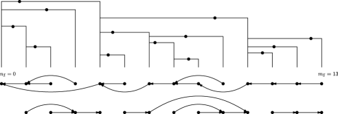
In this section we describe a different way to view invasion percolation which is at the heart of most of the results of this paper. First, imagine keeping notes of the local edge landscape we see as we perform invasion percolation, as follows. At step $i$ of invasion percolation, we explore vertex $v_{i}$ and record the weights of all edges leaving $v_{i}$ and heading into new territory by putting marks on the vertical half-line $\{i\}\times[0,\infty)$ whose heights are the weights of these edges. (When performing invasion percolation on a rooted tree $T$, the edges “heading into new territory” are precisely the edges from $v_{i}$ to its children in $T$.) Running the invasion percolation process until it terminates (or forever) then yields some set $P$ of points in the positive quadrant.

Formally, suppose $G=(V,E)$ is a weighted graph with all edge weights distinct, and with distinguished vertex $v_{0}$. Then the invasion percolation procedure defines an infinite subtree $T$ of $G$, with vertex set $\{v_{0},v_{1},\ldots\}$. For each $i\geq 0$, let $p_{i}(1),p_{i}(2),\ldots,p_{i}(j_{i})$ be the weights of the edges from $v_{i}$ to $V\setminus\{v_{0},\ldots,v_{i}\}$, in increasing order of weight. Let $P^{i}=P^{i}(G)=\{(i,p_{i}(j))\}_{j=1}^{j_{i}}$, and let $P=P(G)=\bigcup_{i=0}^{|V|-1}P^{i}$.

In general, it is not possible to reconstruct the steps taken by invasion percolation by considering only the set $P$. However, this is possible for invasion percolation on trees, and we now explain how. In order to do so, we introduce an inductive procedure for building a tree, given a set of points $P\subset\mathbb{R}^{2}$ and an interval $\mathcal{I}\subset\mathbb{Z}$ of consecutive integers. We write $n_{\mathcal{I}}=\inf\{n\in\mathcal{I}\}\geq-\infty$ and $m_{\mathcal{I}}=\sup\{n\in\mathcal{I}\}\leq\infty$.

For notational convenience, given $X\subseteq\mathbb{R}^{2}$, we write $|X|_{P}$ for $|P\cap X|$. Also, for a point $p\in\mathbb{R}^{2}$, we write $x(p)$ for the $x$-coordinate and $y(p)$ for the $y$-coordinate. Let us assume the following: [1.]

All points of $P$ lie in the upper half-plane. No bounded set contains unboundedly many points.

For any $n\in\mathcal{I}$, there exists $k>0$ with $n-k>n_{\mathcal{I}}-1$ for which $|[n-k,n)\times[0,\infty)|_{P}\geq k$.

|P((-∞,∞)×{y})|≤1 for any $y\in\mathbb{R}$. If $P$ satisfies these three conditions, we say it is reasonable (or $\mathcal{I}$-reasonable, if $\mathcal{I}$ is not clear from context). (Here, as well as later, we state deterministic requirements for the point set $P$; these requirements—and therefore, the results derived from them—will hold almost surely for all the random point sets we consider. In particular, the reader will always be safe thinking of $P$ as a Poisson point set of intensity one in the upper half-plane.) We start from an empty set $P_{n_{\mathcal{I}}}=\varnothing$, from which we will build an increasing sequence of subsets of $\mathcal{N}_{0}$. The following procedure requires $n_{\mathcal{I}}>-\infty$.

0:  For each $i=n_{\mathcal{I}},n_{\mathcal{I}}+1,\ldots,m_{\mathcal{I}}$:

0:  1. Let $p_{i+1}=p_{i+1}(P,\mathcal{I})$ be the point of $([n_{\mathcal{I}},i+1)\times[0,\infty))\cap(P\setminus P_{i})$

0:    minimizing $y(p_{i+1})$.

0:  2. Let $P_{i+1}=P_{i+1}(P,\mathcal{I})=P_{i}\cup\{p_{i+1}\}$, and let $e_{i+1}=e_{i+1}(P,\mathcal{I})=(i+1,$

0:    $\lfloor x(p_{i+1})\rfloor)$.

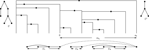
We refer to this procedure as point set invasion percolation. Since $P$ is reasonable, the procedure is well defined. The resulting graph $\operatorname{IPC}(P,\mathcal{I})$ has vertex set $\mathcal{I}$ and edge set $\{e_{i}\dvtx n_{\mathcal{I}}<i<m_{\mathcal{I}}+1\}$. (We write $i<m_{\mathcal{I}}+1$ instead of $i\leq m_{\mathcal{I}}$ since we may have $m_{\mathcal{I}}=\infty$, but $i$ is always finite.) An example is shown in Figure 1. Note that $\operatorname{IPC}(P,\mathcal{I})$ is a tree, which we view as rooted at $n_{\mathcal{I}}$. We often also view $\operatorname{IPC}(P,\mathcal{I})$ as a weighted tree in which edge $e_{i}$ has weight $y(p_{i})$. In general in this section we work in the deterministic setting. However, since our eventual aim is to link this work to invasion percolation on randomly weighted trees we briefly discuss how this can be done.

Figure 1: Top, an $\mathcal{I}$-reasonable set of points $P$, with $\mathcal{I}=\{0,\ldots,13\}$, and the corresponding boxes (defined in Definition 6). Middle, the tree $\operatorname{IPC}(P,\mathcal{I})$. Bottom, the forest $\mathrm{BG}(P,\mathcal{I})$, defined at the start of Section 2.2. All arrows point from child to parent.

IPC of the PWIT

Now suppose that $\mathcal{T}$ is an instance of the PWIT, and let $\mathcal{T}_{0}$ be the subtree of $\mathcal{T}$ explored by invasion percolation. The following lemma is then immediate.

Lemma 4

$\operatorname{IPC}(P(\mathcal{T}),\mathbb{N})$ and $\mathcal{T}_{0}$ are identical, and for each $i\in\mathbb{N}$, $w(e_{i})=y(p_{i})$.

When performing invasion percolation on $\mathcal{T}$, for all $i$, $P^{i}(\mathcal{T})$ is a Poisson point process of rate $1$ on the vertical half-line $\{i\}\times[0,\infty)$, and $P(\mathcal{T})$ is the union of these point processes.

We remark that since all points in $P$ have integer $x$-coordinates, the floor in step 2, above, has no effect. The use of the floor is to ensure that if a point $p=(x,y)\in P$ is replaced by a point $p^{\prime}=(x^{\prime},y)$, as long as $\lfloor x\rfloor=\lfloor x^{\prime}\rfloor$, the resulting graph $\operatorname{IPC}(P,\mathcal{I})$ will be unchanged. As a result we obtain the following corollary.

Corollary 5

Let $\mathcal{P}$ be a Poisson point process of rate $1$ on $[0,\infty)\times[0,\infty)$. Then $\operatorname{IPC}(\mathcal{P},\mathbb{N})$ and $\mathcal{T}_{0}$ are identically distributed.

Associate to each point $p=(x(p),y(p))$ of $P(\mathcal{T})$ an independent uniform $U_{p}$, and let $p^{\prime}$ be the point $(x(p)+U_{p},y(p))$. Then $P^{\prime}=\{p^{\prime}\dvtx p\in P\}$ is a Poisson point process of rate $1$ on $[0,\infty)\times[0,\infty)$, and $\operatorname{IPC}(\mathcal{P}^{\prime},\mathbb{N})$ and $\operatorname{IPC}(P,\mathbb{N})$ are identical. The result follows.

This corollary reduces the study of the distributional properties of $\mathcal{T}_{0}$ to that of the distributional properties of $\operatorname{IPC}(\mathcal{P},\mathbb{N})$, where $\mathcal{P}$ is a Poisson point process of rate $1$ on $[0,\infty)\times[0,\infty)$.

We also demonstrate how the two examples of invasion percolation described in Section 1 can be encoded by suitable point processes.

IPC of an infinite randomly weighted $\sigma$-regular tree

Let $\mathcal{T}_{\sigma}$ be the rooted regular tree with forward degree $\sigma\geq 2$. We can model invasion percolation on $\mathcal{T}_{\sigma}$ as follows: for each $n\in\mathcal{I}=\mathbb{N}$, choose $\sigma$ independent, uniformly random points of $[n,n+1)\times[0,\sigma)$ (or of $\{n\}\times[0,\sigma)$). Let $P$ be the union of all these points.

The minimum spanning tree of the complete graph

Let $K_{\sigma+1}$ be the complete graph on $\sigma+1$ vertices. We may approximately model invasion percolation on a randomly weighted $K_{\sigma+1}$ as follows: for each $n\in\mathcal{I}=\{0,\ldots,\sigma\}$, choose $\sigma-n$ independent, uniformly random points from the set $[n,n+1)\times[0,\sigma)$. Let $P$ be the union of all these points.

This representation is not exact due to the cycles in $K_{n}$. For example, it is possible that the second least weight leaving the starting vertex is on the edge between the second and third vertices visited by Prim’s algorithm. However, the probability of events of this type is asymptotically negligible for the first $o(\sqrt{\sigma})$ steps of the algorithm.

The acyclicity of trees is what allows us to model them by a point process without reference to the order of exploration of vertices. In general—for invasion percolation on $\mathbb{Z}^{d}$, for example—it may still be possible to use some of the following methodology while jointly constructing the point process $P$ and the exploration process “as we go.” However, we have not pursued this avenue of study.

For the remainder of the section, we explore what properties we can derive about the point process invasion percolation procedure with as few restrictions on the point set $P$ as possible. The next definitions and lemma provide an alternative geometric characterization of the connection rule used in the above inductive procedure, one that will be useful throughout the paper.

Definition 6.

Given an interval $\mathcal{I}$, with $n_{\mathcal{I}}>-\infty$, and an $\mathcal{I}$-reasonable point set $P$, for each $i\in\mathcal{I}$ with $i>n_{\mathcal{I}}$, let

$$h_{i}(P,\mathcal{I})=\inf\{h\dvtx\exists j\in\mathcal{I},n_{\mathcal{I}}\leq j<i\mbox{ such that }|[j,i)\times[0,h]|_{P}\geq i-j\}.$$

Let $\ell_{i}(P,\mathcal{I})$ be the minimum integer $\ell_{i}\in[n_{\mathcal{I}},i)$ such that $|[\ell_{i},i)\times[0,h_{P,\mathcal{I}}(i)]|_{P}=i-\ell_{I}$, let $B_{i}(P,\mathcal{I})=[\ell_{i},i)\times[0,h_{i}]$ and let $t_{i}(P,\mathcal{I})$ be the unique point in $B_{i}$ with $y(t_{i})=h_{i}$.

We often omit reference to the parameters $P$ and $\mathcal{I}$ if the context is clear.

We take a moment to observe that these functions are well defined. It follows from condition 2 that $h_{i}$ is finite, and from condition 1 that it is positive. The minimality of $h_{i}$ then implies the existence of a point $p\in P(B_{i})$ such that $y(p)=h_{i}$. The fact there is a unique such point follows from condition 3.

Lemma 7

If $n_{\mathcal{I}}>-\infty$ and $P$ is $\mathcal{I}$-reasonable, then for all $n\in\mathcal{I}\setminus\{n_{\mathcal{I}}\}$, we have $t_{n}=p_{n}$.

It suffices to show (by condition 3) that $y(t_{n})=y(p_{n})$. We prove this by induction on $n$. Clearly, the assertion holds for $n=n_{\mathcal{I}}+1$. Assume $n>n_{\mathcal{I}}+1$ and that $t_{i}=p_{i}$ for all $n_{\mathcal{I}}+1\leq i<n$. First, since $|B_{n}|_{P}=n-\ell_{n}$ and $\bigcup_{i=n_{\mathcal{I}}+1}^{n-1}p_{i}$ contains at most $n-\ell_{n}-1$ points of $P\cap B_{n}$, the set $(P\setminus P_{n-1})\cap B_{n}$ contains at least one point and so $y(p_{n})\leq y(t_{n})$.

To show that $y(t_{n})\leq y(p_{n})$, first note that if $x(p_{n})\geq n-1$, then $|[n-1,\break n)\times[0,y(p_{n})]|_{P}\geq 1$ and so certainly $y(t_{n})\leq y(p_{n})$. We thus assume that $x(p_{n})<n-1$ and construct a sequence $\{a_{i}\}_{i=0}^{k}$ inductively as follows:

0:   Let $i=0$ and let $a_{0}=n-1$.

0:  1. If $a_{i}\leq x(p_{n})$, set $k=i$ and stop.

0:  2. Otherwise, let $a_{i+1}=\ell_{a_{i}}$, then let $i=i+1$ and return to 1.

For each $0\leq i\leq k$ for which $a_{i}$ is defined, if $a_{i}>x(p_{n})$, then $y(p_{a_{i}})<y(p_{n})$ or else the point $p_{n}$ was a better choice for $p_{a_{i}}$. By the inductive hypothesis, $p_{a_{i}}=t_{a_{i}}$. By construction, $|B_{a_{i}}|_{P}=a_{i}-\ell_{a_{i}}=a_{i}-a_{i+1}$ for all $i<k$. Since $B_{a_{i}}\cap B_{a_{j}}=\varnothing$ for all $i\neq j$, we conclude that $\bigcup_{i=0}^{k-1}B_{a_{i}}$ has $n-1-a_{k}$ points of $P$. Thus, $|[a_{k},n)\times[0,y(p_{n})]|_{P}\geq|\{p_{n}\}\cup\bigcup_{i=0}^{k-1}B_{a_{i}}|_{P}\geq n-a_{k}$. By the choice of $h_{n}$ minimum, it follows that $h_{n}=y(t_{n})\leq y(p_{n})$ as required.

The structure of the containment relations among the boxes $B_{i}$ turns out to be interesting in its own right, and we explore aspects of it here as well as later in the paper.

Lemma 8

If $n_{\mathcal{I}}>-\infty$ and $P$ is $\mathcal{I}$-reasonable, then for $n\in\mathcal{I}\setminus\{n_{\mathcal{I}}\}$, either $h_{\ell_{n}}>h_{n}$ or $\ell_{n}=n_{\mathcal{I}}$.

Assume $\ell_{n}\neq n_{\mathcal{I}}$, suppose $h_{\ell_{n}}\leq h_{n}$ and write $m=\ell_{n}$. Then both $B_{m}$ and $B_{n}$ are contained in $[\ell_{m},n)\times[0,h_{n}]$, so $|[\ell_{m},n)\times[0,h_{n}]|_{P}\geq n-\ell_{m}$. This contradicts either the choice of $h_{n}$ or the choice of $\ell_{n}$.

Lemma 9

If $n_{\mathcal{I}}>-\infty$ and $P$ is $\mathcal{I}$-reasonable, then for any $i,j\in\mathcal{I}\setminus\{n_{\mathcal{I}}\}$ with $i<j$, either $B_{i}\cap B_{j}=\varnothing$ or $B_{i}\subseteq B_{j}$.

Suppose that $B_{i}\cap B_{j}\neq\phi$. In particular this implies $\ell_{j}<i$. We prove that $B_{i}\subseteq B_{j}$ by proving that $h_{i}<h_{j}$ and $\ell_{j}\leq\ell_{i}$.

The minimality of $h_{j}$ implies that $|[\ell_{j},j)\times[0,h_{j})|_{P}=j-\ell_{j}-1$ and that $|[i,j)\times[0,h_{j})|_{P}\leq j-i-1$. Thus $|[\ell_{j},i)\times[0,h_{j})|\geq i-\ell_{j}$, which immediately implies that $h_{i}<h_{j}$.

We now prove $\ell_{j}\leq\ell_{i}$. Suppose that $\ell_{i}<\ell_{j}$. Then, by reasoning as above, and using the fact that $h_{j}>h_{i}$ we have that $|[\ell_{i},\ell_{j})\times[0,h_{j})|_{P}\geq|[\ell_{i},\ell_{j})\times[0,h_{i})|_{P}\geq\ell_{j}-\ell_{i}$. This implies that $|[\ell_{i},j)\times[0,h_{j})|_{P}\geq j-\ell_{i}$, which contradicts the definition of $\ell_{j}$.

Lemma 10

If $n_{\mathcal{I}}>-\infty$ and $P$ is $\mathcal{I}$-reasonable, then for any $i,j\in\mathcal{I}\setminus\{n_{\mathcal{I}}\}$ such that $\ell_{j}<i\leq j$, there is a path in $\operatorname{IPC}(P,\mathcal{I})$ between $i$ and $\ell_{j}$.

Observe that since $\ell_{j}<i$, $B_{i}\subset B_{j}$ by Lemma 9. We apply induction on $i-\ell_{j}$. If $i-\ell_{j}=1$, then we must have $\lfloor x(p_{i})\rfloor=\ell_{j}$, so $e_{i}=(i,\ell_{j})$, verifying the claim.

For larger values of $i-\ell_{j}$, first note that since $B_{i}\subset B_{j}$, we must have $\ell_{j}\leq\ell_{i}\leq\lfloor x(p_{i})\rfloor<i$. If $\ell_{j}=\lfloor x(p_{i})\rfloor$, then $e_{i}$ is a path from $i$ to $\ell_{j}$. Otherwise, $\lfloor x(p_{i})\rfloor-\ell_{j}<i-\ell_{j}$, so by induction there is a path from $\lfloor x(p_{i})\rfloor$ to $\ell_{j}$, which together with edge $e_{i}$ yields a path from $i$ to $\ell_{j}$.

2.1 Point process invasion percolation in the upper half-plane

For suitable point sets $P$, we may hope to define a version of the invasion percolation procedure in which $\mathcal{I}=\mathbb{Z}$ (or more generally when $n_{\mathcal{I}}=-\infty$). This is indeed possible, and the resulting infinite graph can be said to capture the behavior of invasion percolation “very far from the root.” A direct inductive description of the graph seems difficult, and so we define the object $\operatorname{IPC}(P,\mathbb{Z})$ as the limit of $\operatorname{IPC}(P,\mathbb{Z}\cap[m,\infty))$ as $m\to-\infty$. Later, we shall also see how the alternative characterization of the connection rule given by Definition 6 and Lemma 7 can be used to define this extension of the invasion percolation procedure.

As before, we desire as few restrictions on $P$ as possible. In this section, we suppose we are given a set of points $P\subset\mathbb{R}^{2}$ and an interval $\mathcal{I}$ with $n_{\mathcal{I}}\geq-\infty$ and $m_{\mathcal{I}}\leq\infty$. We say that $P$ is seemly (or $\mathcal{I}$-seemly, if $\mathcal{I}$ is not clear from context) if $P$ satisfies conditions 1–3 and additionally either (a) $n_{\mathcal{I}}>-\infty$, or (b) $n_{\mathcal{I}}=-\infty$ and $P$ satisfies conditions 4 and 5, below. [4.]

For any $n\in\mathcal{I}$, there are infinitely many $m\in\mathcal{I}\cap(-\infty,n)$ such that $|[m,n)\times[0,1]|_{P}>n-m$.

If $\lambda<1$, then for any $n\in\mathcal{I}$ there are at most finitely many $m\in\mathcal{I}\cap(-\infty,n)$ such that $|[m,n)\times[0,\lambda]|_{P}\geq n-m$. The reader can verify that the following two examples almost surely produce seemly point sets.

Stationary limit of IPC on $\mathcal{T}_{\sigma}$

Let $P$ be defined by choosing $\sigma$ independent, uniformly random points in the set $[n,n+1)\times[0,\sigma)$ for each $n\in\mathcal{I}=\mathbb{Z}$.

Stationary limit of the Poisson IPC

Let $P$ be a Poisson point process of intensity $1$ in the upper half plane, and let $\mathcal{I}=\mathbb{Z}$.

The following lemma essentially states that for $\mathcal{I}$-seemly point sets with $n_{\mathcal{I}}=-\infty$, all edges have weight less than $1$.

Lemma 11

If $n_{\mathcal{I}}=-\infty$ and $P$ is $\mathcal{I}$-seemly, then for any $n\in\mathcal{I}$ there exists $m_{0}\in\mathcal{I}$ such that $h_{n}(P,\mathcal{I}\cap[m,\infty))<1$ for all integers $m\leq m_{0}$.

By condition 4, $|[m,n)\times[0,1]|_{P}>n-m$ for infinitely many integers $m<n$; therefore, $h_{n}(P,\mathcal{I}\cap[m,\infty))<1$ for infinitely many integers $m<n$. But $h_{n}(P,\mathcal{I}\cap[m,\infty))=y(p_{n}(P,\mathcal{I}\cap[m,\infty)))$, and $y(p_{n}(P,\mathcal{I}\cap[m,\infty)))$ is nonincreasing as $m$ decreases, so by condition 3 $y(p_{n}(P,\mathcal{I}\cap[m,\infty)))<1$ for all $m$ small enough.

We next consider the family of intervals $\mathcal{I}\cap[m,\infty)$ for $m\in\mathbb{Z}$, and show that as $m\to-\infty$, each vertex only changes its parent a finite number of times. This allows us to consistently define the limiting object $\operatorname{IPC}(P,\mathcal{I})$.

Lemma 12

If $P$ is $\mathcal{I}$-seemly, then for any $n\in\mathcal{I}$, there exists $m_{0}>-\infty$ such that $p_{n}(P,\mathcal{I}\cap[m,\infty))=p_{n}(P,\mathcal{I}\cap[m_{0},\infty))$ for all $m\in\mathcal{I}\cap(-\infty,m_{0}]$.

The lemma is obvious if $n_{\mathcal{I}}>-\infty$ so assume $n_{\mathcal{I}}=-\infty$. Fix $n\in\mathcal{I}$ and suppose the assertion of the lemma fails for this $n$. Then there exists a strictly decreasing integer sequence $\{m_{i}\}_{i=0}^{\infty}$ and a sequence $\{q_{i}\}_{i=0}^{\infty}$ of distinct points in $P$ such that $p_{n}(P,\mathcal{I}\cap[m_{i},\infty))=q_{i}$ for all $i\in\mathbb{N}$, whose $y$-coordinates decrease strictly as $i$ increases. By Lemma 11, there exists some $i_{0}$ such that $y(q_{i})<1$ for all $i\geq i_{0}$. But then for all $i\geq i_{0}$, $B_{n}(P,\mathcal{I}\cap[m_{i},\infty))\subset[\ell_{n}(P,\mathcal{I}\cap[m_{i},\infty)),n)\times[0,y(q_{i})]$, and so for such $i$,

$$\bigl{|}\bigl{[}\ell_{n}\bigl{(}P,\mathcal{I}\cap[m_{i},\infty)\bigr{)},n\bigr{)}\times[0,y(q_{i})]\bigr{|}_{P} \geq \bigl{|}B_{n}\bigl{(}P,\mathcal{I}\cap[m_{i},\infty)\bigr{)}\bigr{|}_{P}$$

$$\geq n-\ell_{n}\bigl{(}P,Z\cap[m_{i},\infty)\bigr{)}.$$

This is a contradiction to condition 5.

For a seemly point set $P$, we now define $\operatorname{IPC}(P,\mathcal{I})$ to be the graph with vertex set $\mathcal{I}$ and such that for each $n\in\mathcal{I}$, $e_{n}=e_{n}(P,\mathcal{I})=\lim_{m\to-\infty}e_{n}(P,\mathcal{I}\cap[m,\infty))$. This limit is well defined by the preceding lemma. We likewise define $p_{n}(P,\mathcal{I})$, $\ell_{n}(P,\mathcal{I})$, $h_{n}(P,\mathcal{I})$ and $B_{n}(P,\mathcal{I})$. By a limiting argument Lemmas 8, 9 and 10 are also valid with respect to $\operatorname{IPC}(P,\mathcal{I})$ when $n_{\mathcal{I}}=-\infty$. We therefore obtain the following theorem.

Theorem 13

If $P$ is $\mathcal{I}$-seemly, then $\operatorname{IPC}(P,\mathcal{I})$ is a tree.

Since it is clearly acyclic, we just need to show that $\operatorname{IPC}(P,\mathcal{I})$ is connected. Suppose $i,j\in\mathcal{I}$, $i<j$. Let $\ell_{j}^{0}=\ell_{j}$ and for $t\geq 1$, $t\in\mathbb{N}$, let $\ell^{t}_{j}=\ell_{\ell^{t-1}_{j}}$. Then there must exist $t\in\mathbb{N}$ such that $i\in B_{\ell^{t}_{j}}$. By Lemma 10, there is a path between $j$ and $\ell^{t+1}_{j}$, and there is a path between $i$ and $\ell^{t+1}_{j}$. As $i$ and $j$ were arbitrary, this completes the proof.

An advantage of the current formulation of invasion percolation is that we can equivalently define the limit process via conditions on the numbers of points in boxes $[m,n)\times[0,h]$. More precisely, the following lemma is easily verified.

Lemma 14

Suppose $P$ is $\mathcal{I}$-reasonable. Fix $k,n$ with $n_{\mathcal{I}}<k<m_{\mathcal{I}}+1$ and $0<n<(k-n_{\mathcal{I}})+1$, and $y>0$. In order that $\ell_{k}=k-n$ and that $h_{0}=y$, it is necessary and sufficient that the following three conditions hold:

• $|[k-n,k)\times[0,y]|_{\mathcal{P}}=n$ and $|[k-n,k)\times[0,y)|_{\mathcal{P}}=n-1$ [call this condition $E=E(k-n,k,y,P)$].

• For all $0<m\leq n$, $|[k-m,k)\times[0,y)|_{\mathcal{P}}<m$ [call this condition $F=F(k-n,k,y,P)$].

• For all $m\in\mathbb{N}$, $|[k-n-m,k-n)\times[0,y]|_{\mathcal{P}}<m$ [call this condition $G=G(k-n,y,P)$].

In this case, $B_{k}=[k-n,k]\times[0,y]$, $p_{n}$ is the unique point $p\in P$ with $y(p)=y$, and $e_{n}=(n,\lfloor x(p_{n})\rfloor)$.

We will sometimes have use for the condition $G(k-n,y^{-})$, which is the same as the condition $G$ above but with $[0,y]$ replaced by $[0,y)$. The next lemma provides a condition under which we can determine the behavior to the right of a given integer $n$ without further reference to the behavior of $P$ to the left of $n$. Its proof is obvious and is omitted.

Lemma 15

Suppose $P$ is $\mathcal{I}$-reasonable. Fix $n_{\mathcal{I}}<n<m_{\mathcal{I}}+1$ and $y>0$, let $Q=\{p\in P\dvtx x(p)\geq n,y(p)\leq y\}$ and let $\mathcal{J}=\mathcal{I}\cap\{n,\ldots,\infty\}$. If $G(n,y^{-})$ holds and $Q$ is $\mathcal{J}$-reasonable, then for all $m$ with $n<m<m_{\mathcal{I}}+1$, $\ell_{m}(P,\mathcal{I})=\ell_{m}(Q,\mathcal{J})$, $h_{m}(P,\mathcal{I})=h_{m}(Q,\mathcal{J})$ and $p_{n}(P,\mathcal{I})=p_{n}(Q,\mathcal{J})$.

We will also have use of the following sufficient condition for $Q$ to be reasonable. (Again, the proof is straightforward and is omitted.)

Lemma 16

Let $\mathcal{I},P,k,n$ and $y$ be as in Lemma 14, let $\mathcal{J}=\{k-n,\ldots,k\}$ and let $Q=P\cap([k-n,k]\times[0,y])$. If $E,F$ and $G$ all hold, then $Q=P\cap B_{k}$ and $Q$ is $\mathcal{J}$-reasonable.

2.2 Box graphs

As we saw above, the boxes $B_{n}$ play a useful role in our study of invasion percolation. The boxes can also be seen to capture information about the structure of the point process invasion percolation procedure itself. For example, it is easily checked that if the procedure explores some edge $e$ lying within a box $B_{n}$, then it will explore all other edges lying within $B_{n}$ before exploring any edges with an endpoint outside of $B_{n}$. (Of course, the procedural interpretation does not exist when $\mathcal{I}=\mathbb{Z}$, but in this case we can still think of the boxes as capturing information about the process behavior “far from the root.”)

In this section, we introduce a graph which characterizes the containment relation among the boxes. Given an $\mathcal{I}$-reasonable point set $P$, we define $\mathrm{BG}(P,\mathcal{I})$ to be the graph with vertex set $\mathcal{I}\setminus\{n_{\mathcal{I}},+\infty\}$ and such that, for $i<j$, $i$ and $j$ are joined by an edge if and only if $B_{i}(P,\mathcal{I})\subseteq B_{j}(P,\mathcal{I})$ and $B_{i}(P,\mathcal{I})\not\subseteq B_{j^{\prime}}(P,\mathcal{I})$ for any $i<j^{\prime}<j$. Also, for $i\in\mathcal{I}\setminus\{n_{\mathcal{I}},m_{\mathcal{I}}\}$, we write $a_{i}(P,\mathcal{I})$ for the parent of $i$ in $\mathrm{BG}(P,\mathcal{I})$.

Figure 2: The leftmost and middle sets of points have the same $\mathrm{BG}$ graphs but different $\operatorname{IPC}$ graphs. The middle and rightmost sets of points have the same $\operatorname{IPC}$ graph but different $\mathrm{BG}$ graphs.

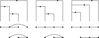
The examples shown in Figure 2 demonstrate that between the graphs $\operatorname{IPC}(P,\mathcal{I})$ and $\mathrm{BG}(P,\mathcal{I})$, neither is determined by the other. [Theorem 1(c) is essentially a consequence of this fact.]

Clearly, $\mathrm{BG}(P,\mathcal{I})$ is acyclic for any $\mathcal{I}$. We shall show that $\mathrm{BG}(P,\mathbb{Z})$ is a tree (i.e., connected) under the additional assumption of the “rightward version” of condition 5.

[6.]

If $\lambda<1$, then for any $m\in\mathcal{I}$, there are at most finitely many $n\in\mathbb{Z}\cap(m,\infty)$ such that $|[m,n)\times[0,\lambda]|_{P}\geq n-m$.

If $P$ satisfies conditions 1–6 with $\mathcal{I}=\mathbb{Z}$, we say that $P$ is exemplary. Both examples of the last subsection are almost surely exemplary point sets.

Lemma 17

Suppose $m_{\mathcal{I}}=\infty$ and $P$ is an $\mathcal{I}$-reasonable point set that satisfies condition 6. Choose any $m\in\mathcal{I}\setminus\{n_{\mathcal{I}},+\infty\}$ for which $h_{m}<1$ and for which there is no $m^{\prime}\in\mathbb{Z}\cap(m,\infty)$ such that $B_{m}\subseteq B_{m}^{\prime}$ and $h_{m}^{\prime}\geq 1$. Then there are infinitely many $n\in\mathbb{Z}\cap(m,\infty)$ such that $B_{m}\subseteq B_{n}$.

Suppose $m$ is as in the statement of the lemma but that there are only finitely many $n>m$ such that $B_{m}\subseteq B_{n}$. Then by replacing $B_{m}$ with the tallest box that contains it, we may assume that in fact there is no $n>m$ such that $B_{m}\subseteq B_{n}$. By condition 6, we may choose $n>m$ for which $|[m,n)\times[0,h_{m}]|_{P}<n-m$. Thus, there must be $i\in\{m+1,\ldots,n\}$ for which $h_{i}>h_{m}$, so take $i$ minimum such that this holds. By Lemma 8, we must then have $\ell_{i}<m$, and so by Lemma 9 we must have $B_{m}\subset B_{i}$, a contradiction.

Before showing that $\mathrm{BG}(P,\mathbb{Z})$ is a tree, let us first use the lemma to confirm the basic property of exemplary point sets that every point of $P$ under the line $y=1$ lies along the top of some box $B_{n}$.

Proposition 18

If $P$ is exemplary, then for all $p\in P\cap[n_{\mathcal{I}},+\infty)\times[0,1)$, we have $p=p_{n}$ for some $n\in\mathcal{I}$.

Let $p\in P$ have $y(p)<1$. We first note that if $p\in B_{m}$ for some $m$, then $p=p_{n}$ for some $\lceil x(p)\rceil\leq n\leq m$. Also, there must be some integer $k\leq x(p)$ for which $h_{k}>y(p)$, or else $|[\lceil x(p)\rceil-i,\lceil x(p)\rceil]\times[0,y(p)]|_{P}\geq i$ for infinitely many integers $i>0$, which contradicts condition 5.

By Lemma 11, $h_{m}<1$ for all $m\in\mathbb{Z}$, so by Lemma 17, there are infinitely many $m\in\mathbb{Z}$ for which $B_{k}\subseteq B_{m}$. One of these boxes contains $p$, so $p=p_{n}$ for some $n$, as claimed.

Theorem 19

If $P$ is exemplary, then $\mathrm{BG}(P,\mathbb{Z})$ is a tree.

It suffices to show that $\mathrm{BG}(P,\mathbb{Z})$ is connected. Recall that $h_{n}<1$ for any $n\in\mathbb{Z}$, by Lemma 11. Fix $i<j$, $i,j\in\mathbb{Z}$. By Lemma 17 there are infinitely many $m$ such that $B_{i}\subset B_{m}$. Take the least such $m$ for which $m\geq i$—then also $B_{j}\subseteq B_{m}$, and so by Lemma 10 there exist paths from $i$ to $m$ and from $j$ to $m$. The theorem follows.

2.3 Random walks and the forward maximal process

Let $P$ be a point set satisfying condition 1. Given $h>0$ and $k\in\mathcal{I}$, we define random walks $S^{k,h}=S^{k,h}(P)$ and $L^{k,h}=L^{k,h}(P)$ as follows. We set $S^{k,h}_{0}=L^{k,h}_{0}=0$ and, for $i\geq 1$, set $S^{k,h}_{i}=|[k,k+i]\times[0,h]|_{P}-i$, and set $L^{k,h}_{i}=|[k,k-i]\times[0,h]|_{P}-i$. We also define random walks $S^{k,h^{-}}$ and $L^{k,h^{-}}$, by replacing $[0,h]$ by $[0,h)$ in the above definitions. In other words, the random walks $S^{k,h^{-}}$ and $L^{k,h^{-}}$ ignore points on the line $y=h$. (For fixed $h$, for any of the random point sets $P$ we will consider, it will be the case that with probability $1$, $S^{k,h}_{i}=S^{k,h^{-}}_{i}$ for all $i$, but we will at times work in conditional settings in which these two random walks are not identical.)

We say that $S^{k,h}$ survives if for all $i\geq 0$, $S^{k,h}_{i}\geq 0$, and otherwise say that $S^{k,h}$ dies. Also, we say that $S^{k,h}$ has a chance if $S^{k,h}_{i}\geq 0$ for some $i>0$, and otherwise that $S^{k,h}$ has no chance. We extend these definitions to $L^{k,h}$ by symmetry.

We now establish two more basic properties of $\operatorname{IPC}(\mathcal{P},\mathcal{I})$, under the following additional assumptions.

[7.]

If $\lambda>1$, then for any $m\in\mathbb{Z}$, $S_{n}^{m,\lambda}\leq n$ for at most finitely many $n\in\mathbb{N}$.

Sk,1 dies for all $k\in\mathcal{I}$. Roughly speaking, condition 7 is a “rightward version” of condition 4. If $P$ is an $\mathcal{I}$-reasonable point set that satisfies conditions 6, 7 and 8, we say that $P$ is distinguished (or $\mathcal{I}$-distinguished, if $\mathcal{I}$ is not clear from context). The first two examples given in the introduction to this section are almost surely distinguished point sets.

We will see that for distinguished point sets $P$, when $n_{\mathcal{I}}>-\infty$ and $m_{\mathcal{I}}=\infty$, $\mathrm{BG}(P,\mathcal{I})$ is not connected—in this case we call the connected components the ponds of $\mathrm{BG}(P,\mathcal{I})$. We will see later that this agrees with the normal use of this term in the invasion percolation literature.

Lemma 20

If $n_{\mathcal{I}}>-\infty$, $m_{\mathcal{I}}=\infty$ and $P$ is $\mathcal{I}$-distinguished, then for any $m\in\mathcal{I}\setminus\{n_{\mathcal{I}},+\infty\}$, if $h_{m}\geq 1$, then there are at most finitely many $n\in\mathbb{Z}$, $n>m$, such that $B_{m}\subseteq B_{n}$.

Suppose otherwise. Without loss of generality, we may assume that $h_{m}>1$. Consider the integer sequence $\{n_{i}\}_{i=0}^{\infty}$, which is defined as follows. Let $n_{0}=m$. For $i\in\mathbb{N}$, let $n_{i+1}$ be the smallest integer greater than $n_{i}$ such that $B_{n_{i}}\subseteq B_{n_{i+1}}$. Then for any $i\in\mathbb{N}$ and all $n_{i}<n<n_{i+1}$, we have $B_{n}\subseteq[n_{i},n_{i+1})\times[0,h_{n_{i}}]$ for all $n_{i}<n<n_{i+1}$ by Lemmas 8 and 9. Furthermore, it follows from the definition of $B_{n}$ and Lemma 9 that $|([n_{i},n_{i+1})\times[0,h_{n_{i+1}}))\setminus(\bigcup_{n_{i}<n<n_{i+1}}B_{n})|_{P}=0$ (or otherwise there would be a smaller choice for $h_{n_{i+1}}$). Thus, $|[n_{i},n_{i+1})\times[0,h_{n_{i}}]|_{P}=|\bigcup_{n_{i}<n<n_{i+1}}B_{n}|_{P}=n_{i+1}-n_{i}-1$. Since $h_{n_{0}}<h_{n_{i}}$ for all $i>0$, it follows that $|[n_{0},n_{i+1})\times[0,h_{n_{0}}]|_{P}<n_{i+1}-n_{0}$ for all $i>0$. Since $h_{n_{0}}>1$, this is a contradiction to condition 7.

Theorem 21

If $n_{\mathcal{I}}>-\infty$, $m_{\mathcal{I}}=\infty$ and $P$ is $\mathcal{I}$-distinguished, then $\mathrm{BG}(P,\mathcal{I})$ contains infinitely many components, all of which are finite. Furthermore, for any given component, if $n$ is the rightmost integer belonging to the component, then $h_{n}>1$ and the set of vertices of the component is $\{\ell_{n}+1,\ldots,n\}$.

Let $P$ satisfy the hypothesis of the theorem. We construct a sequence of integers $\{n_{i}\}_{i=0}^{\infty}$ as follows. Let $n_{0}=n_{\mathcal{I}}$. For $i\in\mathbb{N}$, let $n_{i+1}$ be the largest integer greater than $n_{i}$ such that $B_{n_{i+1}}$ contains the point $(n_{i},0)$. We must now show this sequence is well defined. Suppose not, and let $i$ be minimum such that there is no valid choice for $n_{i+1}$. Then there are infinitely many integers $n>n_{i}$ such that $B_{n_{i}}\subseteq B_{n}$. Since $i$ was chosen minimum, for each such $n$ we have $\ell_{n}=n_{i}$. By Lemma 20, it must be that for each such $n$, $h_{n}<1$. But this implies that $|[n_{i},n)\times[0,1]|_{P}\geq n-n_{i}$ for all $n\in\mathbb{Z}\cap[n_{i},\infty)$, a contradiction to condition 8. Thus the sequence $\{n_{i}\}_{i=0}^{\infty}$ is well defined.

For all $i\in\mathbb{N}$, it follows from the definition of $n_{i+1}$ that $\ell_{n_{i+1}}=n_{i}$, and there is no integer $n>n_{i+1}$ for which $B_{n_{i+1}}\subseteq B_{n}$; thus $B_{n_{i+1}}$ and $B_{n_{i+2}}$ are in separate components of $\mathrm{BG}(P,\mathcal{I})$. By Lemma 9, all $B_{n}$ such that $n_{i}<n\leq n_{i+1}$ are contained in $B_{n_{i+1}}$ and hence in the same component of $\mathrm{BG}(P,\mathcal{I})$.

If $h_{n_{i+1}}<1$ for some $i\in\mathbb{N}$, then by Lemma 17, there are infinitely many $n\in\mathbb{Z}\cap(n_{i+1},\infty)$ such that $B_{n_{i+1}}\subseteq B_{n}$, but this is a contradiction to the choice of $n_{i+1}$. By Lemma 8, we have for all $i\in\mathbb{N}$ that $h_{n_{i+1}}>h_{n_{i+2}}$. We conclude that $h_{n_{i+1}}>1$ for all $i\in\mathbb{N}$.

Given an interval $\mathcal{I}$, with $n_{\mathcal{I}}>-\infty$ and $m_{\mathcal{I}}=\infty$, and an $\mathcal{I}$-distinguished point set $P$, define $\{n_{i}\}_{i=0}^{\infty}=\{n_{i}(P,\mathcal{I})\}_{i=0}^{\infty}$ as in the proof of Theorem 21.

Corollary 22

If $n_{\mathcal{I}}>-\infty$, $m_{\mathcal{I}}=\infty$ and $P$ is $\mathcal{I}$-distinguished, then $\operatorname{IPC}(P,\mathcal{I})$ is a tree that consists of a unique infinite backbone (i.e., a unique, infinite, self-avoiding path originating from the root) from which emerge finite branches. Furthermore, the backbone contains the points $\{n_{i}\}_{i=0}^{\infty}$.

Clearly, $\operatorname{IPC}(P,\mathcal{I})$ is acyclic, and is connected by Lemma 10, so is a tree. For each integer $i\geq 1$, let $\Phi_{i}$ be the unique path from $n_{i}$ to $n_{0}=n_{\mathcal{I}}$ in $\operatorname{IPC}(P,\mathcal{I})$. By Lemma 10, it follows that for all $i\geq 1$, $\Phi_{i}$ is a sub-path of $\Phi_{i+1}$, and so the limit $\Phi=\lim_{i\to\infty}\Phi_{i}$ is a well-defined infinite path starting from $n_{\mathcal{I}}$. Furthermore, for any integer $k$, any path $\Phi^{\prime}$ starting from $v_{k}$, that is, edge-disjoint from $\Phi$ must have all its elements among $n_{i},\ldots,n_{i+1}-1$, where $n_{i}\leq v_{k}<n_{i+1}$. Thus, all branches leaving $\Phi$ are finite.

In general, relaxing any of the conditions in the definition of distinguished point sets may cause the conclusions of Corollary 22 to fail. To provide just one example, the following point set satisfies conditions 1–7, but not the conclusion of Corollary 22. The point set $P$ contains no points except the following. Place $k$ points inside $[0,1)\times[0,1/3)$. Place each of the points $(i+1,1-1/(i+2))$ for $i\in\mathbb{N}$. Then $\operatorname{IPC}(P,\mathbb{N})$ has $k$ infinite backbones.

This completes our study of deterministic properties of the invasion percolation procedure. In the next section we begin our study of what happens when the underlying point set is random.

3 Invasion percolation on the PWIT

Throughout Section 3, $\mathcal{P}$ denotes a Poisson process of constant intensity $1$ in $[0,\infty)\times[0,\infty)$, so $\mathcal{P}$ is almost surely $\mathbb{N}$-distinguished. By Corollary 5, $\operatorname{IPC}(\mathcal{P},\mathbb{N})$ is distributed as the invasion percolation cluster $\mathcal{T}_{0}$ of the PWIT, so results for $\operatorname{IPC}(\mathcal{P},\mathbb{N})$ apply to $\mathcal{T}_{0}$ mutatis mutandis. Below, we will derive more precise statements about the structure of $\operatorname{IPC}(\mathcal{P},\mathbb{N})$ than can be made under the assumptions of Section 2. First, however, we state two “ballot-style” theorems for stochastic processes that we will use repeatedly.

3.1 Two ballot-style theorems

The following result was proved independently by Tanner tanner61derivation and Dwass dwass62fluctuation .

Lemma 23 ((Cycle lemma))

Suppose that $X_{1},\ldots,X_{n}$ are integer-valued, cyclically interchangeable random variables with maximum value $1$. Then for any integer $0\leq k\leq n$,

$$\mathbf{P}\{S_{i}>0\ \forall 1\leq i\leq n\mid S_{n}=k\}=\frac{k}{n}.$$

The next result was proved by Tákacs takacs67comb , page 12.

Lemma 24 ((Stationary ballot theorem))

Let $X_{1},X_{2},\ldots$ be an infinite sequence of i.i.d. integer random variables with mean $\mu$ and maximum value $1$, and for any $i\geq 1$, let $S_{i}=X_{1}+\cdots+X_{i}$. Then

$${\mathbf{P}}\bigl{\{}S_{n}>0\ \forall n\in\{1,2,\ldots\}\bigr{\}}=\cases{\mu,&\quad$\mbox{if }\mu>0,$\vspace*{2pt}\cr 0,&\quad$\mbox{if }\mu\leq 0.$}$$

Now let $P$ be a random point set in, say, $[m,n]\times[0,\infty)$. We recall the definition of the condition $F(m,n,y)$ from Lemma 14, and will abuse notation by also writing $F(m,n,y,P)$ for the event that the condition $F(m,n,y,P)$ holds. [At times we write $F(m,n,y)$ in place of $F(m,n,y,P)$, when $P$ is clear from context.] Notice that if $P$ is a uniform set of $n-1$ points in $[0,n]\times[0,\lambda)$, for some $\lambda>0$, then applying the cycle lemma with $X_{i}=1-|[i-1,i)\times[0,\lambda)|_{P}$ (and so $S_{i}=i-|[0,i)\times[0,\lambda)|_{P}$) for $i=1,\ldots,n$, it follows that the probability that $F(0,n,\lambda,P)$ occurs is precisely $1/n$. By an argument of a similar nature, we can straightforwardly derive the following lemma (which can also be deduced from an existing result (mcdiarmid97mst , Theorem 4) for invasion percolation on $K_{n}$ and a limiting argument).

Lemma 25

Fix an integer $n\geq 1$, and list the $n$ elements of $\mathcal{P}\cap([0,n]\times[0,\infty))$ of lowest height as $q_{1},\ldots,q_{n}$, in increasing order of height. Then for each $i=1,\ldots,n$, ${\mathbf{P}}\{p_{n}=q_{i}\}=1/n$.

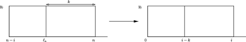
We emphasize that the $n$ elements of $\mathcal{P}\cap([0,n]\times[0,\infty))$ of lowest height may not all be elements of the set $\{p_{1},\ldots,p_{n}\}$, or indeed of the set $\{p_{i}\}_{i=1}^{\infty}$. Proof of Lemma 25 Fix $n$, and let $\lambda=y(q_{n})$. Clearly, $p_{n}$ will be among $q_{1},\ldots,q_{n}$. Also, let $\mathcal{I}=\{0,\ldots,n\}$, let $P=\{q_{1},\ldots,q_{n}\}$ and for each $i\in\{0,\ldots,n-1\}$, let $P^{i}=\{q_{1}^{i},\ldots,q_{n}^{i}\}$ be the cyclic shift of $P$ to the right by distance $i$. Then for all $i\in\{1,\ldots,n-1\}$, $P^{i}$ is distributed as $n-1$ uniform points in $[0,n]\times[0,\lambda)$, together with a single uniform point of height $\lambda$. We claim that with probability $1$, for each $j=1,\ldots,n$, there is exactly one $i=i(j,P)\in\{0,\ldots,n-1\}$ for which $p_{n}(P^{i},\mathcal{I})=q_{j}^{i}$. Since the $P^{i}$ are identically distributed it follows from this claim that

$${\mathbf{P}}\{p_{n}(P,\mathcal{I})\!=\!q_{j}\}=\frac{1}{n}\sum_{i=0}^{n-1}{\mathbf{P}}\{p_{n}(P^{i},\mathcal{I})\!=\!q_{j}^{i}\}=\frac{1}{n}{\mathbf{P}}\Biggl{\{}\bigcup_{i=0}^{n-1}\{p_{n}(P^{i},\mathcal{I})\!=\!q_{j}^{i}\}\Biggr{\}}=\frac{1}{n},$$

which proves the theorem. It thus remains to prove the above claim, which we do by contradiction. Thus, suppose that for some $j\in\{1,\ldots,n\}$, there are distinct $i,i^{\prime}\in\{0,\ldots,n-1\}$ for which $p_{n}(P^{i},\mathcal{I})=q_{j}^{i}$ and $p_{n}(P^{i^{\prime}},\mathcal{I})=q_{j}^{i^{\prime}}$. By replacing $P$ by either $P^{n-i}$ or $P^{n-i^{\prime}}$ if necessary, we may assume that $i^{\prime}=0$. Let $q_{j}=q_{j}^{0}=(x_{j},y_{j})$. We must have $|[n-i,n]\times[0,y_{j})|_{P}<i$ [or else $p_{n}(P,\mathcal{I})\neq q_{j}$]; on the other hand, $|[\ell_{n}(P,\mathcal{I}),n]\times[0,y_{j}]|_{P}=n-\ell_{n}(P,\mathcal{I})$.

Let $k=n-\ell_{n}(P,\mathcal{I})$, the length of $B_{n}(P,\mathcal{I})$. If $k\geq i$, then we also have $|[\ell_{n},n-i]\times[0,y_{j}]|_{P}\geq n-\ell_{n}-i+1$, so $|[\ell_{n}+i,n]\times[0,y_{j}]|_{P^{i}}\geq n-\ell_{n}-i+1$ and $h_{n}(P^{i},\mathcal{I})<y_{j}$, contradicting the fact that $p_{n}(P^{i},\mathcal{I})=q_{j}^{i}$. It follows that $k<i$, that is, that $i-(n-\ell_{n})\geq 1$. In this case, we have that for each $m\in\{1,\ldots,i-(n-\ell_{n})\}$, $[\ell_{n}-m,\ell_{n}]\times[0,y_{j}]<m$ (or else we would have either chosen $h_{n}$ lower or $\ell_{n}$ smaller). Translating the above information to $P^{i}$, we see that $|[i-k,i]\times[0,y_{j}]|_{P^{i}}=k$, that $|[i-k,i]\times[0,y_{j})|_{P^{i}}<k$, and that $|[i-k^{\prime},i]\times[0,y_{j}]|_{P^{i}}<k^{\prime}$ for each $k^{\prime}\in\{k+1,\ldots,i\}$ (see Figure 3). Thus, by Definition 6 and Lemma 7, $p_{i}(P^{i},\mathcal{I})=q_{j}^{i}$, contradicting the assumption that $p_{n}(P^{i},\mathcal{I})=q_{j}^{i}$.

Figure 3: The region on the left maps onto the region on the right when $P$ is sent to $P^{i}$.

We next elaborate on a connection between Poisson Galton–Watson trees and queueing theory that will be useful for many subsequent calculations.

3.2 A fact from queuing theory and an aside on Poisson Galton–Watson duality

The following basic result was first noted by Borel borel1942etb . Consider a queue with Poisson rate $\lambda$ arrivals and constant, unit service time, started at time zero with a single customer in the queue, and with any arbitrary servicing rule (i.e., not necessarily first-in first-out). We may form a rooted tree associated with the queueing process run until the first time $\tau$ that there are no customers in the queue (or forever, if the queue is never empty), in the following manner. If a new customer joins the queue at time $t$, he is joined to the customer being served at time $t$. We denote the resulting rooted tree by $\mathcal{T}$. Then $\mathcal{T}$ is distributed as a Poisson($\lambda$) Galton–Watson tree [we write $\operatorname{PGW}(\lambda)$, for short] borel1942etb .

If the arrival times are given by the $x$-coordinates of the points of Poisson process $\mathcal{Q}=\mathcal{P}\cap([0,\infty)\times[0,\lambda))$, we may also associate an interpolated random walk to the process, by setting $S_{t}=|[0,t)\times[0,\lambda)|_{\mathcal{Q}}-t$ for $t\in\mathbb{R}^{+}$. Then $|\mathcal{T}|$ is simply the first time $t$ that $S_{t}=-1$, that is, that $|[0,t)\times[0,\lambda)|_{\mathcal{Q}}=t-1$. Note that given that $|T|=m<\infty$, $\mathcal{Q}$ is distributed as $m-1$ independent uniform points in $[0,t)\times[0,\lambda]$, conditioned on $F(0,n,\lambda,\mathcal{Q})$ occurring. We also observe that for all $i\leq|\mathcal{T}|$, $S_{i}=S^{0,\lambda^{-}}_{i}$, where $S^{0,\lambda^{-}}$ is the random walk defined in Section 2.3. This has immediate implications for the events defined in Section 2.3. In particular, the tree $\mathcal{T}$ is infinite if and only if $S^{0,\lambda^{-}}$ survives. It follows that for all $0\leq h\leq 1$ we have ${\mathbf{P}}\{S^{k,\lambda^{-}}\mbox{ survives}\}=0$, and for all $\lambda>1$ we have ${\mathbf{P}}\{S^{k,\lambda^{-}}\mbox{ survives}\}=\theta(\lambda)$, the probability of survival of a $\operatorname{PGW}(\lambda)$ branching process. Similarly, by Lemma 24, we have that the probability that there is ever a time $t$ at which the total number of arrivals is at least $t$, is $\min(\lambda,1)$. Thus, if $0<\lambda\leq 1$, then ${\mathbf{P}}\{S^{k,\lambda^{-}}\mbox{ has a chance}\}=\lambda$, and if $\lambda>1$ then ${\mathbf{P}}\{S^{k,\lambda^{-}}\mbox{ has a chance}\}=1$. Of course, the exact same identities hold with $S^{k,\lambda^{-}}$ replaced by $S^{k,\lambda}$, $L^{k,\lambda^{-}}$ or $L^{k,\lambda}$.

We continue to think of arrival times as given by points of $\mathcal{Q}$. It will be useful for us to view the above queuing procedure as creating a tree whose nodes are labeled by integers rather than by elements of the queue. We do so by re-labeling each node of $\mathcal{T}$ (i.e., each customer $c$) with the (integer) time at which $c$ begins being served. Furthermore, suppose that we take as our servicing rule the invasion percolation rule—that is, the rule that prioritizes customers (points of $\mathcal{Q}$) with lower $y$-coordinate over those with higher $y$-coordinate—and call the resulting tree $\mathcal{T}_{\lambda}$. Then $\mathcal{T}_{\lambda}$ is precisely the subtree of $\operatorname{IPC}(\mathcal{P},\mathbb{N})$ containing the root and all nodes joined to the root by paths all of whose edges have weight less than $\lambda$. Of course, everything still holds if we take $\mathcal{Q}=\mathcal{P}\cap([0,\infty)\times[0,\lambda])$—that is, if we include points at height precisely $\lambda$—as long as we replace $S^{0,\lambda-}$ by $S^{0,\lambda}$ and replace the phrase “less than $\lambda$” by “at most $\lambda$.”

As a consequence of the above discussion we have the following important fact.

Lemma 26

Fix any integer $n\geq 1$, any $\lambda>0$, and let $P$ be a set of $n-1$ independent uniform points in $[0,n]\times[0,\lambda)$. Given that $F(0,n,\lambda,P)$ occurs, the tree $\operatorname{IPC}(P,\{0,\ldots,n-1\})$ is distributed as $\operatorname{PGW}(\lambda)$ conditioned to have $n$ nodes. Furthermore, suppose that $p$ is a uniformly random point on the line segment $[0,n]\times\{\lambda\}$. Then under the same conditioning, $\operatorname{IPC}(P\cup\{p\},\{0,\ldots,n\})$ is distributed as $\operatorname{PGW}(\lambda)$ conditioned to have $n$ nodes, together with an additional vertex (vertex $n$), joined to a uniformly random element of $0,\ldots,n-1$.

We remark that for any fixed $n$, the distribution of $\operatorname{PGW}(\lambda)$ conditioned to have $n$ nodes does not depend on $\lambda$ and is precisely that of a uniformly random labelled rooted tree (or Cayley tree) on $n$ nodes, after the labels but not the orders of children have been discarded. It turns out that a version of Lemma 26 also holds for the box tree; see Lemma 37, below. As noted just after Lemma 24, the probability that $F(0,n,\lambda,P)$ occurs is precisely $1/n$. Thus, the distribution of $|\operatorname{PGW}(\lambda)|$ is given by

$${\mathbf{P}}\{|\operatorname{PGW}(\lambda)|=n\}=\frac{1}{n}{\mathbf{P}}\{\operatorname{Poisson}(\lambda n)=n-1\}=\frac{e^{-\lambda n}(\lambda n)^{n-1}}{n!},$$

for all positive integers $n$ (a well-known fact which we record for later reference). When $\lambda=1$ this is called the Borel distribution.

We briefly explain a further basic fact about the function $\theta(\lambda)=\break{\mathbf{P}}\{|\operatorname{PGW}(\lambda)|=\infty\}$ and about Poisson Galton–Watson duality. By considering the number of children in the first generation of $\operatorname{PGW}(\lambda)$, we see that $1-\theta(\lambda)=e^{-\lambda\theta(\lambda)}$, and by differentiating this identity, we see that

$$\theta^{\prime}(\lambda)\bigl{(}1-\lambda\bigl{(}1-\theta(\lambda)\bigr{)}\bigr{)}=\theta(\lambda)\bigl{(}1-\theta(\lambda)\bigr{)},$$ (1)

an equation we will have use of later. Next, given $\lambda>1$, let $m=m(\lambda)<1$ be such that $\lambda e^{-\lambda}=me^{-m}$ (we call $m$ the dual parameter for $\lambda$). Then $m=\lambda(1-\theta(\lambda))$, from which it is easily seen that conditional on being finite, $\operatorname{PGW}(\lambda)$ is distributed precisely as $\operatorname{PGW}(m)$.

3.3 $\operatorname{IPC}(\mathcal{P},\mathbb{N})$ and the forward maximal process

By Corollary 22,$\operatorname{IPC}(\mathcal{P},\mathbb{N})$ consists of a unique infinite backbone which in particular passes through the nodes $\{n_{i}\}_{i=0}^{\infty}$, and from all nodes of which emerge finite branches. Let the edges of the backbone be $e_{1},e_{2},\ldots,$ and for each integer $i\geq 1$ let $W_{i}=\sup_{j\geq i}W_{e_{j}}$, so $\{W_{i}\}_{i=1}^{\infty}$ is the PWIT forward maximal process. From the perspective of the PWIT, the nodes $n_{i}$ are the nodes at which the forward maximal weight along the backbone decreases.

Lemma 26 allows us to provide another picture of the structure of$\operatorname{IPC}(\mathcal{P},\mathbb{N})$. First, for each integer $i\geq 0$, let $T_{i}=T_{i}(\mathcal{P},\mathbb{N})$ be the subtree of $\operatorname{IPC}(\mathcal{P},\mathbb{N})$ on nodes $n_{i},\ldots,n_{i+1}-1$ (these nodes induce a tree by Lemma 10). The set $P=\mathcal{P}\cap([n_{i},n_{i+1})\times[0,h_{n_{i+1}}))$ is distributed as $(n_{i+1}-n_{i}-1)$ independent uniform points, conditional on $F(n_{i},n_{i+1},h_{n_{i+1}},P)$ occurring. Furthermore, $\mathcal{P}\cap([n_{i},n_{i+1})\times\{h_{n_{i+1}}\})$ contains a single uniform point. Thus, by Lemma 26, we obtain that $T_{i}$ is distributed as $\operatorname{PGW}(h_{n_{i+1}})$ conditioned to have $n_{i+1}-n_{i}$ nodes, and that $n_{i+1}$ is joined to a uniformly random element of $T_{i}$. Applying this for all $i$, we obtain the following theorem.

Theorem 27

Given $\{n_{i}\}_{i=0}^{\infty}$, $\operatorname{IPC}(\mathcal{P},\mathbb{N})$, viewed as an unlabeled tree, can be built as follows. For each integer $i\geq 0$ let $T_{i}$ be a uniformly random labeled tree on $n_{i}-n_{i-1}$ vertices. For each integer $i\geq 1$, join the root of $T_{i}$ to a uniformly random vertex of $T_{i-1}$. Finally, discard all labels.

It also follows straightforwardly from Lemma 26 that given $\{n_{i}\}_{i=0}^{\infty}$ and $\{h_{n_{i+1}}\}_{i=0}^{\infty}$, $\operatorname{IPC}(\mathcal{P},\mathbb{N})$ viewed as a weighted unlabeled tree can be built from the tree described in Theorem 27 as follows. Independently for each integer $i\geq 0$ and each edge $e$ of $T_{i}$, assign $e$ a random weight with $\operatorname{Uniform}[0,h_{n_{i+1}}]$ distribution. Also, for each integer $i\geq 0$, give the unique edge from $T_{i+1}$ to $T_{i}$ the weight $h_{n_{i+1}}$. We omit the details.

We next show that $\{(|T_{i-1}|,h_{n_{i}})\}_{i=1}^{\infty}=\{(n_{i}-n_{i-1},h_{n_{i}})\}_{i=1}^{\infty}$ is a Markov process and specify the transition probabilities. First, for any $i\geq 1$, given $h_{n_{i}}$, the set $\mathcal{Q}=\mathcal{P}\cap([n_{i},\infty)\times[0,h_{n_{i}}))$ is precisely a Poisson point process of intensity $1$ conditioned on the event that $S^{n_{i},h_{n_{i}^{-}}}(\mathcal{Q})$ survives (which is precisely the event that $\mathcal{Q}$ is $\{n_{i},n_{i+1},\ldots,\}$-reasonable). Furthermore, given $h_{n_{i}}$, the condition $G(n_{i},h_{n_{i}}^{-})$ holds for $\mathcal{P}$. Thus, by Lemma 15, we can determine the structure of $\operatorname{IPC}(\mathcal{P},\mathbb{N})$ restricted to $\{n_{i},\ldots,\infty\}$ by considering only the points in $\mathcal{Q}$. It follows that $\{(n_{i}-n_{i-1},h_{n_{i}})\}_{i=1}^{\infty}$ is a Markov process, as claimed (and also that $\{h_{n_{i}}\}_{i=1}^{\infty}$ is a Markov process). Next, for $1<y<h$, let

$$f_{h}(y)=\lim_{dy\to 0}\frac{\mathbf{P}\{h_{n_{i+1}}\in dy\mid h_{n_{i}}=h\}}{dy},$$

and for $n>0$ let

$$f_{h}(n,y)=\lim_{dy\to 0}\frac{\mathbf{P}\{h_{n_{i+1}}\in dy,(n_{i+1}-n_{i})=n\mid h_{n_{i}}=h\}}{dy},$$

so $f_{h}(y)=\sum_{n}f_{h}(n,y)$. By the above comments, $f_{h}(y)$ and $f_{h}(n,y)$ do not depend on $i$.

Lemma 28

For all $i\geq 1$ and $1<y<h$,

$$f_{h}(y)=\frac{\theta^{\prime}(y)}{\theta(h)}\quad\mbox{and}\quad f_{h}(n,y)=\frac{\theta(y)}{\theta(h)}\frac{e^{-yn}(yn)^{n-1}}{(n-1)!}.$$

Combining the two results in Lemma 28, the following corollary is immediate.

Corollary 29

For all integers $n,i\geq 1$ and $y>1$,

$$\mathbf{P}\{n_{i+1}-n_{i}=n\mid h_{n_{i+1}}=y\}=\frac{\theta(y)}{\theta^{\prime}(y)}\frac{e^{-ny}(ny)^{n-1}}{(n-1)!}.$$ (2)

Proof of Lemma 28 We have

$$\mathbf{P}\{h_{n_{i+1}}\leq y\mid h_{n_{i}}=h\} = \mathbf{P}\{S^{n_{i},y}(\mathcal{P})\mbox{ survives}\mid S^{n_{i},h^{-}}(\mathcal{P})\mbox{ survives}\}$$

$$= \frac{{\mathbf{P}}\{S^{n_{i},y}(\mathcal{P})\mbox{ survives}\}}{{\mathbf{P}}\{S^{n_{i},h^{-}}(\mathcal{P})\mbox{ survives}\}}$$

$$= \frac{\theta(y)}{\theta(h)},$$

and the first claim of the lemma follows by differentiation.

As mentioned, $f_{h}(y)$ and $f_{h}(n,y)$ do not depend on $i$, so we take $i=0$ (and thus $n_{i}=0$). In order to have $n_{1}-n_{0}=n$ and $h_{n_{1}}\in dy$, we need that $|[0,n]\times[0,y)|_{\mathcal{P}}=n-1$, that $|[0,n]\times[y,y+dy)|_{\mathcal{P}}=1$, that $F(0,n,y,\mathcal{P})$ occurs and that $S^{n,y^{-}}(\mathcal{P})$ survives. The probabilities of the first two events are easily bounded. The probability of $F(0,n,y,\mathcal{P})$ given that $|[0,n]\times[0,y)|_{\mathcal{P}}=n-1$ is $1/n$ by the cycle lemma. Finally, the event that $S^{n,y^{-}}(\mathcal{P})$ survives is independent of the first three events, and has probability $\theta(y)$. Thus,

$$\mathbf{P}\{h_{n_{i+1}}\in dy,(n_{i+1}-n_{i})=n\mid h_{n_{i}}=h\}$$

$$\qquad=\frac{e^{-yn}(yn)^{n-1}}{(n-1)!}\cdot\bigl{(}1+o(dy)\bigr{)}n\,dy\cdot\frac{1}{n}\cdot\theta(y)\cdot\frac{1}{\theta(h)},$$

from which the second claim of the lemma follows.

We next derive the distribution of the distance along the backbone between $n_{i-1}$ and $n_{i}$. For $i\geq 0$ let $d_{i}=d_{i}(\mathcal{P},\mathcal{I})=d_{\operatorname{IPC}}(n_{i},n_{i+1})$. As with the quantities studies above, we have that given $h_{n_{i+1}}$, $d_{i}$ is independent of the past. For $0<x<1$ we say $X\stackrel{{\scriptstyle d}}{{=}}\operatorname{Geometric}(x)$ if ${\mathbf{P}}\{X=k\}=x^{k}(1-x)$.

Theorem 30

For all $i\geq 0$ and all $y>1$, given that $h_{n_{i+1}}=y$, $d_{i}\stackrel{{\scriptstyle d}}{{=}}1+\operatorname{Geometric}(m(y))$.

The following theorem derives the distributions of the trees hanging off the backbone and within a given pond.

Theorem 31

Fix $i\geq 0$ and $y>1$. Given that $h_{n_{i+1}}=y$, for all $k$ with $n_{i}\leq k<n_{i+1}$ and for which $k$ is on the backbone, the subtree of $\operatorname{IPC}(\mathcal{P},\mathbb{N})$ containing $k$ and containing no other vertices of the backbone, is distributed as $\operatorname{PGW}(m(y))$.

Together, Theorems 30 and 31 provide another Markovian characterization of $\operatorname{IPC}(\mathcal{P},\mathbb{N})$: we may construct a tree with the distribution of $\operatorname{IPC}(\mathcal{P},\mathbb{N})$ by growing the trees hanging off the backbone one-by-one, where the branching distribution of the trees depends on the current forward maximal weight. (This characterization is exactly that which is claimed in Theorem 3, which is proved below.) The forward maximal weight process evolves according to the dynamics implied by Lemma 28 and Theorem 30: first stay constant for a geometric amount of time depending on the current forward maximal weight, then decrease the maximal weight according to Lemma 28. This characterization is essentially the $\sigma\to\infty$ limit of results of Angel et al. angel2006ipr described in the Introduction, for invasion percolation on the regular $\sigma$-ary tree. However, it does not seem trivial to derive these results from theirs by a limiting argument and local weak convergence, since they depend not only on the graph structure of the tree but also on the weights.

If one wishes, at this point one can apply all the methodology of angel2006ipr to see that corresponding results hold for invasion percolation on the PWIT: notably, convergence to the Poisson lower envelope, mutual singularity of IPC and IIC measures and spectral asymptotics all hold for invasion percolation on the PWIT. We have not included the details as the development is essentially technical, requiring no significant ideas not already found in angel2006ipr .

Since $m(\lambda)=\lambda(1-\theta(\lambda))$, we also obtain the following corollary of Theorems 27, 30 and 31 and Corollary 29, which is new as far as we know. For any $0<p<1$, let $D=\operatorname{Geometric}(p)$, and let $r=v_{0},v_{1},\ldots,v_{D}=v$ be a path of length $D$. For each $k\in\{0,\ldots,D\}e$, starting from $v_{k}$ grow a $\operatorname{PGW}(p)$ tree with root $v_{k}$. This yields a triple $(T,r,v)_{p}$.

Corollary 32

Fix any $0<p<1$ and let $(T,r,v)_{p}$ have the distribution described above. Then conditional on $|T|$, $T$ is distributed as $\operatorname{PGW}(p)$ conditioned to have size $|T|$, and $v$ is distributed as a uniformly random node of $T$. Furthermore, let $y=m^{-1}(p)$. Then for all $n\geq 1$, ${\mathbf{P}}\{|T|=n\}$ is given by the right-hand side of (2).

We now turn to the proof of Theorem 30. Recall that for $y>1$, $m(y)$ is the dual parameter for $y$. We will make use of the following easy (and known) lemma.

Lemma 33

Let $T$ be a Cayley tree of order $n$ with root $r$, and let $v$ be a uniformly random node in $T$. Then

$${\mathbf{P}}\{d_{T}(r,v)=k-1\}=\frac{k(n)_{k}}{n^{k+1}}\vspace*{-3pt}$$

where $(n)_{k}=n(n-1)\cdots(n-k+1)$.

We view $T$ as a doubly-rooted tree with roots $r$ and $v$. By removing the edges on the path from $r$ to $v$, we obtain a forest of $d_{T}(r,v)$ rooted trees, whose roots are ordered (as $r=v_{1},\ldots,v_{k}=v$, say). The number of such forests is $({n\atop k})k!\cdot(kn^{n-k-1})$; see, for example, moon70counting , Theorem 3.2. The result follows by dividing by the total number of doubly-rooted trees on $n$ labeled vertices, which is $n^{n}$ by Cayley’s formula.

Proof of Theorem 30 As mentioned at the start of Section 3.3, for all $i$, $n_{i+1}$ is joined to a uniformly random element of $T_{i}$—say $v_{i}$—and $d_{\operatorname{IPC}}(n_{i},n_{i+1})=1+d_{T_{i}}(n_{i},v_{i})$. By Corollary 29 and Lemma 33, it follows that

$$\mathbf{P}\{d_{\operatorname{IPC}}(n_{i},n_{i+1})=k\mid h_{n_{i+1}}=y\}$$

$$\qquad=\sum_{n=k}^{\infty}\mathbf{P}\{d_{T_{i}}(n_{i},v_{i})=k-1\mid|T_{i}|=n\}\mathbf{P}\{|T_{i}|=n\mid h_{n_{i+1}}=y\}$$

$$\qquad=\sum_{n=k}^{\infty}\frac{k(n)_{k}}{n^{k+1}}\cdot\frac{\theta(y)}{\theta^{\prime}(y)}\frac{e^{-ny}(ny)^{n-1}}{(n-1)!}$$

$$\qquad=y^{k-1}\frac{\theta(y)}{\theta^{\prime}(y)}\sum_{n=k}^{\infty}\frac{k}{n}\cdot\frac{e^{-ny}(ny)^{n-k}}{(n-k)!}$$

$$\qquad=y^{k-1}\frac{\theta(y)}{\theta^{\prime}(y)}\sum_{n=k}^{\infty}\frac{k}{n}{\mathbf{P}}\{\operatorname{Poisson}(ny)=n-k\}.$$

By the cycle lemma,

$$\frac{k}{n}{\mathbf{P}}\{\operatorname{Poisson}(ny)=n-k\}={\mathbf{P}}\{S_{n}^{0,y}=-k,S_{i}^{0,y}>-k\ \forall 0\leq i<n\},$$

so

$$\mathbf{P}\{d_{\operatorname{IPC}}(n_{i},n_{i+1})=k\mid h_{n_{i+1}}=y\}=y^{k-1}\frac{\theta(y)}{\theta^{\prime}(y)}{\mathbf{P}}\{S_{n}^{0,y}=-k\mbox{ for some }n\}.$$

But by the connection with queueing theory explained above, ${\mathbf{P}}\{S_{n}^{0,y}=-k\mbox{ for}\mbox{some }n\}$ is precisely the probability that $k$ independent $\operatorname{PGW}(y)$ all fail to survive, which is $(1-\theta(y))^{k}$. We complete the proof by applying the identity (1) from page 1.

Proof of Theorem 31 For this theorem we revert to viewing$\operatorname{IPC}(\mathcal{P},\mathbb{N})$ as a subtree of the PWIT $\mathcal{T}$; our proof is based on the proof of Proposition 2.3 of angel2006ipr . Given a node $v\in\mathcal{T}$, write $\mathcal{T}_{v}$ [resp. $\mathcal{T}_{v}(\lambda)$] for the subtree of $\mathcal{T}$ rooted at $v$ (resp. rooted at $v$ and containing all edges of weight at most $\lambda$ to descendants of $v$)—so $\mathcal{T}_{v}(\lambda)\stackrel{{\scriptstyle d}}{{=}}\operatorname{PGW}(\lambda)$—and write $\lambda^{*}(v)=\inf\{\lambda\dvtx\mathcal{T}_{v}(\lambda)\mbox{ is infinite}\}$.

Let $r$ be the root of $\mathcal{T}$, and fix any node $v\in\mathcal{T}$. Fix $y>1$ and integers $1\leq j\leq k$. Let $E_{v,j,k,dy}$ be the event that $v$ is on the backbone, has $k$ children of whom the backbone passes through the $j$th (in the left-to-right ordering of the PWIT) and $\lambda^{*}(v)\in dy$. We split $E_{v,j,k,dy}$ into four events depending on distinct edge sets of the PWIT:

1. [$F_{1}$]

2. $\mathcal{T}_{r}(y)-\mathcal{T}_{v}(y)$ is finite. (This event depends only on edges of $\mathcal{T}-\mathcal{T}_{v}$.)

3. $v$ has precisely $k$ children of weight at most $y+dy$—say $v_{1},\ldots,v_{k}$. (This depends only on the weights of edges from $v$ to its children.)

4. For $i\in\{1,\ldots,k\}\setminus\{j\}$, $\mathcal{T}_{v_{i}}(y+dy)$ is finite. (This depends only on the weights edges in the subtrees $\mathcal{T}_{v_{i}}$ for $i\neq j$.)

5. $\mathcal{T}_{v_{j}}(y)$ is finite, but $\mathcal{T}_{v_{j}}(y+dy)$ is infinite. (This depends only on the weights of edges in $\mathcal{T}_{v_{j}}$.)

Since the edge sets determining the events $F_{1},\ldots,F_{4}$ are disjoint, if $E$ occurs, then the conditioning on subtrees $\mathcal{T}_{v_{i}}(y)$ for $i\in\{1,\ldots,k\}\setminus\{j\}$ is precisely that they are finite. Thus, given that $E$ occurs, for each $i\in\{1,\ldots,k\}\setminus\{j\}$, $\mathcal{T}_{v_{i}}(y)$ is distributed as $\operatorname{PGW}(m(y))$.

Now let $E_{v,dy}=\bigcup_{i,j}E_{v,i,j,dy}$—so $E_{v,dy}$ is the event that $v$ is on the backbone and that $\lambda^{*}(v)\in dy$. Given the observation at the end of the previous paragraph, to prove the theorem it suffices to show that as $dy\to 0$, given $E_{v,dy}$, the number $N_{v}(y+dy)$ of children of $v$ in $\mathcal{T}_{v}(y+dy)$ approaches $\operatorname{Poisson}(m(y))+1$ in distribution [so that the number of children off the backbone approaches $\operatorname{Poisson}(m)$]. To see this is an easy calculation. First,

$${\mathbf{P}}\{E_{v,dy}\} = {\mathbf{P}}\{F_{1}\}\cdot{\mathbf{P}}\{\mathcal{T}_{v}(y)\mbox{ is finite but }\mathcal{T}_{v}(y+dy)\mbox{ is infinite}\}$$

$$= {\mathbf{P}}\{F_{1}\}\cdot\bigl{(}1+o(dy)\bigr{)}\theta^{\prime}(y)\,dy.$$

Next, fixing $k\geq 1$, by symmetry,

$${\mathbf{P}}\{N_{v}(y+dy)=k,E_{v,dy}\}$$

$$\qquad=\bigl{(}1+o(dy)\bigr{)}{\mathbf{P}}\{F_{1}\}\cdot{\mathbf{P}}\{\operatorname{Poisson}(y)=k\}\cdot k\cdot\bigl{(}1-\theta(y)\bigr{)}^{k-1}\cdot\theta^{\prime}(y)\,dy.$$

The factor $k$ above selects which of the $k$ children of $v$ is on the backbone. Since $m=y(1-\theta(y))$, it follows that

$$\lim_{dy\to 0}\mathbf{P}\{N_{v}(y+dy)=k\mid E_{v,dy}\} = {\mathbf{P}}\{\operatorname{Poisson}(y)=k\}\cdot k\cdot\bigl{(}1-\theta(y)\bigr{)}^{k-1}$$

$$= {\mathbf{P}}\{\operatorname{Poisson}(m)=k-1\},$$

which completes the proof.

4 The stationary graph and box processes

Throughout this section, $\mathcal{P}$ denotes a Poisson point process of intensity $1$ in the upper half-plane, so $\mathcal{P}$ is almost surely exemplary and $\mathbb{Z}$-distinguished.

4.1 Rooted subtrees in the box tree

Recall that $\mathrm{BG}=\mathrm{BG}(\mathcal{P},\mathbb{Z})$ is the tree with vertex set $\mathbb{Z}$ defined in Section 2. For $n\in\mathbb{Z}$, we let $\mathrm{BG}^{n}$ denote the subtree of $\mathrm{BG}$ rooted at $n$, and write $|\mathrm{BG}^{n}|$ for its size (number of vertices). By the definition of $\mathrm{BG}$, it is immediate that $|\mathrm{BG}^{n}|=n-\ell_{n}$. Our main aim in this section is to prove the following theorem.

Theorem 34

$\mathrm{BG}(\mathcal{P},\mathbb{Z})$ is distributed as the Poisson IIC, in the local weak sense.

A key step in proving Theorem 34, one that additionally introduces several of the main ideas, is the following theorem.

Theorem 35

For all $n\in\mathbb{Z}$, conditional on $\ell^{n}(\mathcal{P},\mathbb{Z})$ and $h^{n}(\mathcal{P},\mathbb{Z})$, $\mathrm{BG}^{n}(\mathcal{P},\mathbb{Z})$ is distributed as $\operatorname{PGW}(h^{n})$ conditioned to have $n-\ell^{n}$ nodes. Furthermore, unconditionally $\mathrm{BG}^{n}$ is distributed as $\operatorname{PGW}(1)$.

Corollary 36 ((mcdiarmid97mst , Theorem 1))

We have $\lfloor x(p_{0})\rfloor\stackrel{{\scriptstyle d}}{{=}}-\lfloor AV\rfloor$, where $A$ is Borel distributed, and $V$ is $\operatorname{Uniform}[0,1]$ and independent of $A$.

Given $\ell_{0}$ and $h_{0}$, the line segment $[\ell_{0},0]\times\{h_{0}\}$ contains a single uniformly random point, and this point is $p_{0}$. The second assertion of the theorem implies that $\ell_{0}$ is Borel distributed, and the corollary follows.

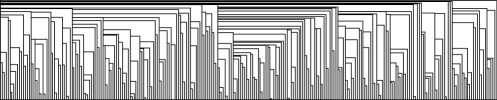
For the next several pages, we focus on developing the tools needed for the proof of Theorem 35. By translation invariance, it suffices to prove Theorem 35 with $n=0$. We prove the theorem by way of the following analog of Lemma 26 that holds for the box tree.

Lemma 37

Let $n$, $\lambda$, $P$ and $p$ be as in Lemma 26. Given that $F(0,n,\lambda,P)$ occurs, $\mathrm{BG}(P\cup\{p\},\{0,\ldots,n\})$ is distributed as $\operatorname{PGW}(\lambda)$ conditioned to have $n$ nodes.

We remark that for any $\lambda>0$, $\operatorname{PGW}(\lambda)$ conditioned to have $k$ nodes and $\operatorname{PGW}(1)$ conditioned to have $k$ nodes are identically distributed. Thus, in proving Theorem 35 and Lemma 37 we may and shall at times assume without loss of generality that $\lambda=1$. Figure 4 contains an example of $\mathrm{BG}(P\cup\{p\},\{0,\ldots,n\})$ for $P$, $p$ as in Lemma 37, with $n=256$. (By the preceding comment, the value of $\lambda$ is not important.) In proving the lemma, it will be important to view $\operatorname{PGW}(1)$ both as an ordered (plane) tree and as an unordered tree. The ordered perspective is natural for $\operatorname{PGW}(1)$ when viewed as a subtree of the PWIT. Next, fix an unordered, rooted tree $U$. We will abuse notation by writing $\operatorname{PGW}(1)=U$ if $\operatorname{PGW}(1)=T$ for some ordered tree $T$ with underlying unordered tree $U$. Fix one such tree $T$, and let $\operatorname{aut}(U)$ be the number of rooted automorphisms of $T$. [Note: by this we mean the number of distinct plane trees with underlying unrooted tree $U$; e.g., for the tree $U$ in Figure 5, interchanging the pair of leaves $x$ and $y$ does not affect the plane tree, and $\operatorname{aut}(U)=12$.] We then have ${\mathbf{P}}\{\operatorname{PGW}(1)=U\}=\operatorname{aut}(T)\cdot{\mathbf{P}}\{\operatorname{PGW}(1)=T\}$.

Figure 4: The boxes for a random set of 256 points. The points themselves are omitted. The code for generating this image was written by Omer Angel.

Figure 5: Viewed as an unordered tree, the above tree has $\mathrm{aut}(U)=12$.

We next turn our attention to $\mathrm{BG}^{0}$. There is again a natural ordering of children in $\mathrm{BG}^{0}$—vertices are integers, and when we refer to a box tree as an ordered tree, we are referring to the ordering inherited from the integers. However, unlike in $\operatorname{PGW}(1)$, we cannot expect the distributions of distinct subtrees to be identical under this ordering. Given an unordered tree $U$, we will also abuse notation by writing ${\mathbf{P}}\{\mathrm{BG}^{0}=U\}$ if $\mathrm{BG}^{0}$ is unlabeled, rooted isomorphic to $U$.

Our proof of Lemma 37 makes use of the following easy fact.

Lemma 38

Let $r\geq 2$ and let $s_{1},\ldots,s_{r}$ be natural numbers. Then

$$\sum_{\pi}\prod_{j=2}^{r}\frac{s_{\pi(j)}}{\sum_{i=1}^{j}s_{\pi(i)}}=1,$$

where the summation is over all permutations $\pi$ of $\{1,\ldots,r\}$.

We proceed by induction on $r$. For $r=2$, the sum is over just two permutations, and the result is

$$\frac{s_{1}}{s_{2}+s_{1}}+\frac{s_{2}}{s_{1}+s_{2}}=1,$$

as required. For general $r$, we partition the set of permutations $\pi$ of $\{1,\ldots,r\}$ depending on the value of $\pi(r)$—for each $k=1,\ldots,r$, let $\Pi_{k}$ be the set of permutations $\pi$ of $\{1,\ldots,r\}$ with $\pi(r)=k$. Since our aim is to prove that the sum

$$\sum_{\pi}\prod_{j=2}^{r}\frac{s_{\pi(j)}}{\sum_{i=1}^{j}s_{\pi(i)}}=\sum_{k=1}^{r}\sum_{\pi\in\Pi_{k}}\prod_{j=2}^{r}\frac{s_{\pi(j)}}{\sum_{i=1}^{j}s_{\pi(i)}}$$

has the value one, it suffices to prove that for each $k$ we have

$$\sum_{\pi\in\Pi_{k}}\prod_{j=2}^{r}\frac{s_{\pi(j)}}{\sum_{i=1}^{j}s_{\pi(i)}}=\frac{s_{k}}{\sum_{i=1}^{r}s_{i}}.$$

Since the expression on the right-hand side here is the $j=r$ term of the product for all $\pi\in\Pi_{k}$, it suffices to show that

$$\sum_{\pi\in\Pi_{k}}\prod_{j=2}^{r-1}\frac{s_{\pi(j)}}{\sum_{i=1}^{j}s_{\pi(i)}}=1.$$

By re-labeling if necessary, this may be deduced from the induction hypothesis.

Proof of Lemma 37 Fix an unordered tree $U$ with $n$ vertices and root $r$. We will show that

$$n\cdot{\mathbf{P}}\{\mathrm{BG}(P,[n])=U\}=\mathbf{P}\{\operatorname{PGW}(1)=U\mid|\operatorname{PGW}(1)|=n\}.$$ (3)

Proving this equality will prove the lemma, since $F(0,n,\lambda,P)$ must occur in order to have $\mathrm{BG}(P,[n])=U$, and ${\mathbf{P}}\{F(0,n,\lambda,P)\}=1/n$ as noted just after Lemma 24. The case $n=1$ of (3) is trivial, so suppose that $n>1$ and that the proposition holds for all $n^{\prime}$ with $1\leq n^{\prime}<n$.

Order the children of the root $r$ of $U$ arbitrarily, and suppose that the subtrees $U_{1},\ldots,U_{k}$ of $U$ rooted at the children of the root have sizes $n_{1},\ldots,n_{k}$ with respect to this order. Let $\operatorname{aut}(r)$ be the number of permutations of the children of $r$ which induce automorphisms of $U$. [For example, the tree in Figure 5 has $\operatorname{aut}(r)=2$.]

We note that

$$\mathbf{P}\{\operatorname{PGW}(1)=U\mid|\operatorname{PGW}(1)|=n\}$$

$$\qquad=\frac{{\mathbf{P}}\{\operatorname{PGW}(1)=U\}}{{\mathbf{P}}\{|\operatorname{PGW}{1}|=n\}}$$

$$\qquad=\frac{n!}{n^{n-1}e^{-n}}\cdot\frac{e^{-1}}{k!}\frac{k!}{\operatorname{aut}(r)}\prod_{i=1}^{k}{\mathbf{P}}\{\operatorname{PGW}(1)=U_{i}\}$$ (4)

$$\qquad=\frac{1}{\operatorname{aut}(r)}\frac{n!}{n^{n-1}}\prod_{i=1}^{k}\frac{n_{i}^{n_{i}-1}}{n_{i}!}\mathbf{P}\{\operatorname{PGW}(1)=U_{i}\mid|\operatorname{PGW}(1)=n_{i}\}$$

$$\qquad=\frac{n}{\operatorname{aut}(r)}\pmatrix{n-1\vspace*{2pt}\cr n_{1},\ldots,n_{k}}\prod_{i=1}^{k}\biggl{(}\frac{n_{i}}{n}\biggr{)}^{n_{i}}\frac{1}{n_{i}}\mathbf{P}\{\operatorname{PGW}(1)=U_{i}\mid|\operatorname{PGW}(1)=n_{i}\}.$$

Next, assume the points of $P$ are listed in increasing order of height as $\{p_{1},\ldots,p_{n}\}$. We first consider the sizes of the subtrees of $B_{0}$.

Let $m_{0}=0$ and for $i=1,\ldots,k$, let $m_{i}=m_{i-1}+n_{i}$ (so in particular $m_{k}=n-1$). Also for $i=1,\ldots,k$, let $Q_{i}$ be the set of points $p\in P\setminus\{p_{n}\}$ satisfying $m_{i-1}\leq x(p)<m_{i}$, and let $p^{i}$ be the point of $Q_{i}$ with greatest $y$-coordinate.

We recall the definitions of the events $E,F$ and $G$ from Lemma 14. In order for $n$ to have children with subtrees $U_{1},\ldots,U_{k}$ in that order, it is necessary and sufficient that the following events occur:

[(III)]

$E(m_{i-1},m_{i},y(p^{i}),P)$ occurs for each $i\in\{1,\ldots,k\}$;

We have $y(p^{i})>y(p^{2})>\cdots>y(p^{k})$;

$F(m_{i-1},m_{i},y(p^{i}),P)$ and $G(m_{i-1},y(p^{i}),P)$ occur for each $i=\{1,\ldots,k\}$;

$\mathrm{BG}^{m_{i}}=U_{i}$ for each $i=\{1,\ldots,k\}$. First, (I) is equivalent to the requirement that $|Q_{i}|=n_{i}$ for each $i=\{1,\ldots,k\}$. The $x$-coordinates of points in $P$, are uniformly distributed on $[-n,0]$ so

$${\mathbf{P}}\{\mbox{(I)}\}=\pmatrix{n-1\vspace*{2pt}\cr n_{1},\ldots,n_{k}}\prod_{i=1}^{k}\biggl{(}\frac{n_{i}}{n}\biggr{)}^{n_{i}}.$$ (5)

Given (I), for (II) to occur it suffices that for each $i=\{1,\ldots,k\}$, the point of $(P\setminus\{p_{n}\})\setminus(Q_{1}\cup\cdots\cup Q_{i-1})$ with the largest $y$-coordinate, is a member of $Q_{i}$. Thus,

$$\mathbf{P}\{\mbox{(II)}\mid\mbox{(I)}\}=\prod_{i=1}^{k}\frac{n_{i}}{n-1-\sum_{j=1}^{i-1}n_{j}}.$$ (6)

Since $y(p^{i})<y(p^{j})$ for $j<i$, if (I), (II) and $\bigcap_{i=1}^{k-1}F(m_{i-1},m_{i},y(p^{i}))$ all hold for some $k\geq 1$, then it is immediate that $G(m_{i-1},y(p^{i}))$ occurs for each $i=\{1,\ldots,k\}$. Thus,

$$\mathbf{P}\{\mbox{(III)}\mid\mbox{(I)},\mbox{(II)}\}=\mathbf{P}\Biggl{\{}\bigcap_{i=1}^{k}F(m_{i-1},m_{i},y^{*}(i))\Bigm{|}\mbox{(I)},\mbox{(II)}\Biggr{\}}.$$

Furthermore, given (I) and (II), independently for each $i=\{1,\ldots,k\}$, the points of $Q_{i}\setminus\{p^{i}\}$ are independently and uniformly distributed in $[m_{i-1},m_{i})\times[0,y(p^{i}))$. Thus, by the cycle lemma,

$$\mathbf{P}\{\mbox{(III)}\mid\mbox{(I)},\mbox{(II)}\}=\prod_{i=1}^{k}\mathbf{P}\{F(m_{i-1},m_{i},y(p^{i}))\mid\mbox{(I)},\mbox{(II)}\}=\prod_{i=1}^{k}\frac{1}{n_{i}}.$$

Finally, given (I), (II) and (III) and independently for each $i=\{1,\ldots,k\}$, $Q_{i}\setminus\{p^{i}\}$ is precisely a uniform set of $n_{i}-1$ points, conditioned on $F(m_{i-1},m_{i},\break y(p^{i}),Q_{i})$ holding, and $p^{i}$ is a uniform point on $[m_{i}-n_{i},m_{i}]\times\{y(p^{i})\}$. Furthermore, by Lemma 15, given $E(m_{i-1},m_{i},y(p^{i}))$, $F(m_{i-1},m_{i},y(p^{i}))$ and $G(m_{i-1},y(p^{i}))$, we have

$$\mathrm{BG}^{m_{i}}(P,\{0,\ldots,n\})=\mathrm{BG}(Q_{i},\{m_{i-1},\ldots,m_{i}\}).$$

Thus, by the induction hypothesis,

$$\mathbf{P}\{\mbox{(IV)}\mid\mbox{(I)},\mbox{(II)},\mbox{(III)}\}$$

$$\qquad=\prod_{i=1}^{k}\mathbf{P}\{\mathrm{BG}^{m_{i}}(P,\{0,\ldots,n\})=U_{i}\mid E(m_{i-1},m_{i},y(p^{i})),$$

$$\qquad\hskip 86.0ptF(m_{i-1},m_{i},y(p^{i})),G(m_{i-1},y(p^{i}))\}$$

$$\qquad=\prod_{i=1}^{k}\mathbf{P}\bigl{\{}\mathrm{BG}(Q_{i},\{m_{i-1},\ldots,m_{i}\})=U_{i}\mid F(m_{i-1},m_{i},y(p^{i}))\bigr{\}}$$

$$\qquad=\prod_{i=1}^{k}\mathbf{P}\{\operatorname{PGW}(1)=U_{i}\mid|\operatorname{PGW}(1)|=n_{i}\}.$$

Combining (5)–(4.1), and rearranging, we obtain that

$${\mathbf{P}}\bigl{\{}n\mbox{ has children }U_{1},\ldots,U_{k}\mbox{ in that order in }\mathrm{BG}(P\cup p,\{0,\ldots,n\}\bigr{\}}$$

$$\qquad=\pmatrix{n-1\vspace*{2pt}\cr n_{1},\ldots,n_{k}}\prod_{i=1}^{k}\frac{n_{i}}{n-1-\sum_{j=1}^{i-1}n_{j}}$$

$$\hskip 72.0pt\qquad{}\times\prod_{i=1}^{k}\biggl{(}\frac{n_{i}}{n}\biggr{)}^{n_{i}}\frac{1}{n_{i}}\mathbf{P}\{\operatorname{PGW}(1)=U_{i}\mid|\operatorname{PGW}(1)|=n_{i}\},$$

$$\qquad=\frac{\operatorname{aut}(r)}{n}\prod_{i=1}^{k}\frac{n_{i}}{n-1-\sum_{j=1}^{i-1}n_{j}}\mathbf{P}\{\operatorname{PGW}(1)=U\mid|\operatorname{PGW}(1)|=n\},$$

the latter equality holding due to (4.1). To obtain ${\mathbf{P}}\{\mathrm{BG}(P\cup p,\{0,\ldots,n\})=U\}$, we now must sum this bound over distinct orderings of $U_{1},\ldots,U_{k}$. We instead sum over all permutations $\pi\dvtx[k]\to[k]$, and note that this counts each distinct ordering $\operatorname{aut}(r)$ times. We thus obtain

$${\mathbf{P}}\bigl{\{}\mathrm{BG}(P\cup p,\{0,\ldots,n\})=U\bigr{\}}$$

$$\qquad=\frac{1}{n}\mathbf{P}\{\operatorname{PGW}(1)=U\mid|\operatorname{PGW}(1)|=n\}\cdot\sum_{\pi\dvtx[k]\to[k]}\prod_{i=1}^{k}\frac{n_{\pi(i)}}{n-1-\sum_{j=1}^{i-1}n_{\pi(j)}}.$$

By Lemma 38, the above sum is 1, which establishes (3) by induction and so completes the proof.

In proving Theorem 35, we will use the following identity, which we quote in advance.

Lemma 39

For integers $a\geq 0$, $b>0$, let $I_{a,b}:=\int_{0}^{1}x^{a}e^{-bx}\,dx$. Then $I_{b-1,b}-I_{b,b}=e^{-b}/b$ for each $b>0$.

Integration by parts.

The final step before proving Theorem 35 is to derive the conditional distribution of $\ell_{0}=|\mathrm{BG}^{0}|$ given $h_{0}$. As this will be useful later in the paper, we state it as a separate lemma. Write

$$\varphi_{y}(n)=\lim_{dy\to 0}\frac{{\mathbf{P}}\{|\ell_{0}|=n,h_{0}\in[y,y+dy)\}}{dy}.$$

Lemma 40

For all $0<y<1$ and all $n\geq 1$,

$$\varphi_{y}(n)=(1-y)\cdot\frac{e^{-ny}(ny)^{n-1}}{(n-1)!}.$$ (8)

Fix $n\in\mathbb{N}$ and $0<y<1$. In order to have $\ell_{0}=-n$ and $h_{0}=y$, it is necessary and sufficient that $E=E(-n,0,y,P),F=F(-n,0,y,P)$ and $G=G(-n,y,P)$, from Lemma 14 all occur. We first calculate the density of the event $E$.

$${\mathbf{P}}\{|[-n,0)\times[0,y)|_{\mathcal{P}}=n-1,|[-n,0)\times[y,y+dy)|_{\mathcal{P}}=1\}$$

$$\qquad=\bigl{(}1+o(dy)\bigr{)}{\mathbf{P}}\{\operatorname{Poisson}(ny)=n-1\}\cdot n\,dy$$

$$\qquad=\bigl{(}1+o(dy)\bigr{)}\frac{e^{-ny}(ny)^{n-1}}{(n-1)!}\cdot n\,dy.$$

Now let $f_{E}(y)=f_{E}(0,n,y)=\frac{e^{-ny}(ny)^{n-1}}{(n-1)!}\cdot n$. Given that $|[-n,0)\times[0,y)|_{\mathcal{P}}=n-1$ occurs, $\mathcal{P}([-n,0]\times[0,y))$ consists of $n-1$ uniformly random points. Independently of this, given that $|[-n,0)\times\{y\}|_{\mathcal{P}}=1$, the line segment $[-n,0]\times\{y\}$ contains a single uniformly random point. By the first of the two preceding observations and by the cycle lemma, it follows that $\mathbf{P}\{F\mid E\}=\frac{1}{n}$. Furthermore, $G$ is independent of $E$, and so by Lemma 24, ${\mathbf{P}}\{G\}=1-y$. We thus have

$$\varphi_{y}(n)=\mathbf{P}\{F,G\mid E\}f_{E}(y)={\mathbf{P}}\{G\}\mathbf{P}\{F\mid E\}f_{E}(y),$$

from which the lemma follows. Proof of Theorem 35 We assume without loss of generality that $n=0$. Let $P=([\ell_{0},0]\times[0,h_{0}])\cap\mathcal{P}$, and let $p=([\ell_{0},0]\times\{h_{0}\})\cap\mathcal{P}$. Then $P$ is precisely distributed as a set of $|\ell_{0}|-1$ uniform points in $([\ell_{0},0]\times[0,h_{0}])$, conditional on $F(\ell_{0},0,h_{0})$, and $p$ has uniform distribution on $([\ell_{0},0]\times\{h_{0}\})$. The first claim of the theorem then follows from Lemma 37. Next, by Lemma 40, for any positive integer $m$ we have

$${\mathbf{P}}\{|\ell_{0}|=m\} = \int_{0}^{1}\varphi_{y}(m)\,dy$$

$$= \frac{m^{m-1}}{(m-1)!}(I_{m-1,m}-I_{m,m}),$$

where the notation $I_{a,b}$ is that defined in Lemma 39. Applying that lemma, we obtain that ${\mathbf{P}}\{|\mathrm{BG}^{0}|=m\}$ is $m^{m-1}e^{-m}/m!$ [exactly the probability that a PGW(1) has size $m$]. The second claim of the theorem then follows from the first and the fact that the conditional distribution of $\operatorname{PGW}(\lambda)$ given its size, is independent of $\lambda$.

Before proving Theorem 34, we first state a consequence of the above development.

Corollary 41

For any positive integer $n$, any $0<y<1$, and any unordered rooted tree $U$ with $|U|=n$,

$$\lim_{dy\to 0}\frac{{\mathbf{P}}\{\mathrm{BG}^{0}=U,h_{0}\in dy\}}{dy}=(1-y)n{\mathbf{P}}\{\operatorname{PGW}(y)=U\}.$$

Immediate from (8) and Theorem 35.

Proof of Theorem 34 We will in fact prove that for any unordered rooted tree $U^{\prime}$, conditional on $\mathrm{BG}^{0}=U^{\prime}$, $\mathrm{BG}^{a_{0}}\setminus\mathrm{BG}^{0}$ is distributed as $\operatorname{PGW}(1)$, which implies the statement of the theorem. Thus, let $U$ and $U^{\prime}$ be unordered rooted trees with roots $r$ and $r^{\prime}$, and let $U^{*}$ be the unordered rooted tree with root $r$ obtained by adding an edge between $r$ and $r^{\prime}$. We define

$$E = \{\mathrm{BG}^{0}=U^{\prime},\mathrm{BG}^{a_{0}}\setminus\mathrm{BG}^{0}=U\}$$

$$= \{\mathrm{BG}^{0}=U^{\prime},\mathrm{BG}^{a_{0}}=U^{*}\}.$$

Next let $k=k(U^{*})$ be the number of children of $r$ in $U^{*}$, and let $j=j(U^{*},U^{\prime})\geq 1$ be the number of children of $r$ in $U^{*}$ whose subtree is isomorphic to $U^{\prime}$. Also, let $\operatorname{aut}(r)$ [resp. $\operatorname{aut}^{*}(r)]$ be the number of permutations of the children of $r$ in $U$ (resp. $U^{*}$) which induce automorphims of $U$ (resp. $U^{*}$). Note that $\operatorname{aut}^{*}(r)=j\cdot\operatorname{aut}(r)$.

Figure 6: In the above figure, an ordering ${\mathbf{u}}=(U_{1},U_{2},U_{3})$ of the children of $U^{*}$ is fixed. Dashed edges lead from $a_{0}$ to its three children. In this example, $j(U^{*},U^{\prime})=2$ since $U_{1}$ and $U_{3}$ are (unordered, rooted) isomorphic to $U^{\prime}$ but $U_{2}$ is not, and $i_{1}({\mathbf{u}})=1$, $i_{2}({\mathbf{u}})=3$ for the same reason. Finally, this example relates to the event $E_{{\mathbf{u}},p}$ with $p=1$, since $a_{0}=m_{i_{1}}({\mathbf{u}})$.

Given an ordering ${\mathbf{u}}=(U_{1},\ldots,U_{k})$ of the children of $r$ in $U^{*}$, let $i_{1}=i_{1}(\mathbf{u}),\ldots,i_{j}=i_{j}(\mathbf{u})$ be the indices $i$ for which $U_{i}$ is isomorphic to $U^{\prime}$. For each $\ell\in\{0,\ldots,k\}$, let $m_{\ell}=m_{\ell}(\mathbf{u})=1+\sum_{q=\ell+1}^{k}|U_{q}|$ (which is $1$ when $\ell=k$). Let

$$E_{{\mathbf{u}}}=E\cap\{a_{0}\mbox{ has children }U_{1},\ldots,U_{k}\mbox{ in that order}\},$$

and for each $p\in\{1,\ldots,j\}$, let

$$E_{{\mathbf{u}},p}=E_{\mathbf{u}}\cap\{a_{0}=m_{i_{p}}(\mathbf{u})\}=\{m_{i_{p}}(\mathbf{u})\mbox{ has children }U_{1},\ldots,U_{k}\mbox{ in that order}\}.$$

(The above definitions are depicted in Figure 6.) Then $E=\bigcup_{\mathbf{u}}\bigcup_{p=1}^{j}E_{{\mathbf{u}},p}$, where the first union is over all distinct orderings $\mathbf{u}$ [we say $\mathbf{u}=(U_{1},\ldots,U_{k})$ and $\mathbf{u}^{\prime}=(U_{1}^{\prime},\ldots,U_{k}^{\prime})$ are distinct if there is some $i\in\{1,\ldots,k\}$ for which $U_{i}$ and $U_{i}^{\prime}$ are not isomorphic]. The double union is then over disjoint terms, and so

$${\mathbf{P}}\{E\}=\sum_{\mathbf{u}}\sum_{p=1}^{j}{\mathbf{P}}\{E_{\mathbf{u},p}\}.$$

Reversing the order of summation above, by translation invariance and Theorem 35, we obtain

$${\mathbf{P}}\{E\} = \sum_{p=1}^{j}\sum_{\mathbf{u}}{\mathbf{P}}\{E_{\mathbf{u},p}\}$$

$$= j\cdot{\mathbf{P}}\{\mathrm{BG}^{0}=U^{*}\}$$

$$= j\cdot{\mathbf{P}}\{\operatorname{PGW}(1)=U^{*}\}.$$

Now fix some ordering $U_{1},\ldots,U_{k}$ of the children of $r$ in $U^{*}$ with $U_{k}=U^{\prime}$. Then by the definition of $\operatorname{PGW}(1)$ and the preceding equality, we have

$${\mathbf{P}}\{E\} = j\cdot\frac{e^{-1}}{k!}\frac{k!}{\operatorname{aut}^{*}(r)}\prod_{i=1}^{k}{\mathbf{P}}\{\operatorname{PGW}(1)=U_{i}\}$$

$$= {\mathbf{P}}\{\operatorname{PGW}(1)=U^{\prime}\}\cdot\frac{e^{-1}}{(k-1)!}\frac{(k-1)!}{\operatorname{aut}(r)}\prod_{i=1}^{k-1}{\mathbf{P}}\{\operatorname{PGW}(1)=U_{i}\}$$

$$= {\mathbf{P}}\{\operatorname{PGW}(1)=U^{\prime}\}{\mathbf{P}}\{\operatorname{PGW}(1)=U\}.$$

It follows by Theorem 35 that

$$\mathbf{P}\{\mathrm{BG}^{a_{0}}\setminus\mathrm{BG}^{0}=U|\mathrm{BG}^{0}=U^{\prime}\} = \frac{{\mathbf{P}}\{E\}}{{\mathbf{P}}\{\mathrm{BG}^{0}=U^{\prime}\}}$$

$$= {\mathbf{P}}\{\operatorname{PGW}(1)=U\},$$

proving the theorem.

4.2 An ancestral process in $\operatorname{IPC}(\mathcal{P},\mathbb{Z})$

By the end of this section we will have proved Theorems 1–3 from the Introduction. To warm up, we prove the following theorem.

Theorem 42

The subtree of $\operatorname{IPC}(\mathcal{P},\mathbb{Z})$ rooted at zero and containing only nodes with positive label, is distributed as $\operatorname{PGW}(1)$.

By Proposition 18, each point of $\mathcal{P}$ in $[0,1]\times[0,1]$ yields a child of $0$ in $T_{0}$, so $0$ has $\operatorname{Poisson}(1)$ children. Let $r_{0}=0$, and let $r_{1}=\min(i>0\dvtx\lfloor x(p_{i})\rfloor=0)$, so $r_{1}$ is “the first integer with $0$ as a parent.” For any $i>0$, the event that $r_{1}=i$ is independent of $\mathcal{P}\cap([i,\infty)\times[0,\infty))$, so $r_{1}$ also has $\operatorname{Poisson}(1)$ children. More generally, let $r_{k}=\min(i>r_{k-1}\dvtx\lfloor x(p_{i})\rfloor\in\{r_{0},\ldots,r_{k-1}\})$. Then for all $k\geq 1$ and all $i>0$, the event that $r_{k}=i$ is independent of $\mathcal{P}\cap([i,\infty)\times[0,\infty))$, so $r_{k}$ has $\operatorname{Poisson}(1)$ children. The nodes $r_{0},r_{1},r_{2},\ldots$ are precisely the descendants of $0$, and we have just seen that each has $\operatorname{Poisson}(1)$ children independently of all the others. This proves the theorem.

Heuristically, the fact that $\operatorname{IPC}(\mathcal{P},\mathbb{Z})$ is equal in distribution to the IIC can be seen as follows. By symmetry, from Theorem 42, at each node of $\operatorname{IPC}(\mathcal{P},\mathbb{Z})$ is rooted a copy of $\operatorname{PGW}(1)$. Also, by exploring the nodes of multiple trees in a left-to-right fashion as in Theorem 42, we see that the offspring distribution for distinct branches of $\operatorname{IPC}(\mathcal{P},\mathbb{Z})$ are independent. Furthermore, the parent of $0$ in $\operatorname{IPC}(\mathcal{P},\mathbb{Z})$ is more likely to be a node with many children than one with few children. This should “size-bias” the number of children of the parent of zero, in such a way as to precisely compensate for the edge from $0$ to its parent, so that a $\operatorname{Poisson}(1)$ number of children remain. The same argument should also hold for the parent of the parent of zero, and so on ad infinitum. It is possible to make (parts of) this heuristic argument rigorous; however, we obtain the result as a relatively direct byproduct of our argument for Theorem 3, whose proof requires a different approach.

The key to the proof is the definition of a “backward maximum process” which is extremely similar to the forward maximal process. We begin by listing $0$ and its ancestors in $\operatorname{IPC}(\mathcal{P},\mathbb{Z})$ in decreasing order as $n_{0},n_{1},n_{2}$, et cetera, so in particular $n_{0}=0$ and in general $n_{i+1}=\lfloor x(p_{n_{i}})\rfloor$. For $i\geq 0$ let $w_{i}=h_{n_{i}}$, and let $m_{i}=\max_{0\leq j\leq i}w_{j}$, the greatest weight of any of the first $(i+1)$ edges. In particular, $m_{0}=w_{0}=h_{0}$. Finally, let $i_{0}=0$ and, for $k\geq 1$, let $i_{k}$ be the smallest integer $i>i_{k-1}$ for which $m_{i_{k}}>m_{i_{k-1}}$. Then the following lemma is basic (but important).

Lemma 43

For all $k\geq 1$, $n_{i_{k}}=\ell(n_{i_{k-1}})$, and so $m_{i_{k}}=h_{n_{i_{k}}}$.

The fact that $n_{i_{k}}\leq\ell(n_{i_{k-1}})$ is immediate from Lemma 9. But $\ell=\ell(n_{i_{k-1}})$ is an ancestor of $n_{i_{k-1}}$ by Lemma 10, and $h_{\ell}>h_{n_{i_{k-1}}}$ by Lemma 8. Thus, $\ell(n_{i_{k-1}})=n_{i_{k}}$ as claimed.

Above, we derived the joint distribution of the height and length of $B_{0}$. We next show that the sequence $\{m_{i_{k}}\}_{k\in\mathbb{N}}$ has a particularly simple and pleasing description.

Lemma 44

The sequence $\{m_{i_{k}}\}_{k\in\mathbb{N}}$ is a homogeneous Markov chain, and for all $k$, given $m_{i_{k}}$, $m_{i_{k+1}}$ has distribution $\operatorname{Uniform}[m_{i_{k}},1]$.

For all $0<y<1$ and all $k$, $h_{k}\leq y$ if and only if the random walk $L^{k,y}$ has a chance. As remarked in Section 3.2, the probability of this is precisely $y$. Given $m_{i_{k-1}}$ and $n_{i_{k}}$, by Lemmas 8 and 43, we know precisely that $m_{i_{k}}=h_{n_{i_{k}}}>h_{n_{i_{k-1}}}=m_{i_{k-1}}$. In other words, we know precisely that the random walk $L^{n_{i_{k}},m_{i_{k-1}}}$ has no chance. Thus, for $0<m<y<1$,

$$\mathbf{P}\{m_{i_{k}}\leq y\mid m_{i_{k-1}}=m\}$$

$$\qquad{}=\mathbf{P}\{h_{n_{i_{k}}}\leq y\mid m_{i_{k-1}}=m\}$$

$$\qquad{}=\mathbf{P}\{L^{n_{i_{k}},y}\mbox{ has a chance}\mid L^{n_{i_{k}},m}\mbox{ has no chance}\}$$

$$\qquad{}=\frac{1-{\mathbf{P}}\{L^{n_{i_{k}},y}\mbox{ has no chance}\}-{\mathbf{P}}\{L^{n_{i_{k}},m}\mbox{ has a chance}\}}{{\mathbf{P}}\{L^{n_{i_{k}},m}\mbox{ has no chance}\}}$$

$$\qquad{}=\frac{y-m}{1-m},$$

which proves the lemma.

Note also, by the first remark in the proof of the lemma, we have the following proposition.

Proposition 45 ((mcdiarmid97mst , Theorem 2))

$h_{0}\stackrel{{\scriptstyle d}}{{=}}\operatorname{Uniform}[0,1]$.

We now prove a more substantial result, about the structure of the portion of $\operatorname{IPC}(\mathcal{P},\mathbb{Z})$ that lives “under the backward maximum process.” It essentially states that, like the forward maximal process, the portion of $\operatorname{IPC}(\mathcal{P},\mathbb{Z})$ that lives under the backward maximum process looks like a single infinite backbone, to which subcritical Poisson Galton–Watson trees are attached at each point. Also, these subcritical trees become closer and closer to critical the further along the backbone from $0$ they are.

Theorem 46

Let $\operatorname{IPC}^{-}(\mathcal{P},\mathbb{Z})$ denote the restriction of $\operatorname{IPC}(\mathcal{P},\mathbb{Z})$ to the nonpositive integers, and let $0$ be its root. Then $\operatorname{IPC}^{-}(\mathcal{P},\mathbb{Z})$ is distributed as $\mathcal{T}_{\mathrm{IIC}}^{*}$.

We will prove this theorem at the end of the section. For each $k\geq 0$, let $\mathcal{P}_{k}=\mathcal{P}\cap([n_{i_{k+1}},n_{i_{k}}]\times[0,m_{i_{k}}))$ and let $\mathcal{I}_{k}=\{n_{i_{k+1}},n_{i_{k+1}}+1,\ldots,n_{i_{k}}\}$. By Lemma 26, given $(n_{i_{k+1}}-n_{i_{k}})$, $\operatorname{IPC}(\mathcal{P}_{k},\mathcal{I}_{k})$ is distributed as $\operatorname{PGW}(m_{i_{k}})$ conditioned to have $(n_{i_{k+1}}-n_{i_{k}})$ nodes, together with a single additional node (the node $n_{i_{k}}$) attached to a uniform vertex.

Theorem 47

For all $k\geq 0$ and $0<m<1$, given that $m_{i_{k}}=m$,$\operatorname{IPC}(\mathcal{P}_{k},\mathcal{I}_{k})$ is distributed as a path with $(1+\operatorname{Geometric}(m))$ edges, from $n_{i_{k+1}}$ to $n_{i_{k}}$, with an independent $\operatorname{PGW}(m)$ tree attached to each node of the path except $n_{i_{k}}$.

The proof uses a correspondence between $\operatorname{IPC}(\mathcal{P}_{k},\mathcal{I}_{k})$ and a pond of $\operatorname{IPC}(\mathcal{P},\mathbb{N})$ of appropriate height. Let $\lambda>1$ be such that $me^{-m}=\lambda e^{-\lambda}$, so then $m=\lambda(1-\theta(\lambda))$. For all $n\geq 1$, by Lemma 40 we have

$$\mathbf{P}\{n_{i_{k+1}}-n_{i_{k}}=n\mid m_{i_{k}}=m\} = (1-m)\cdot\frac{(mn)^{n-1}e^{-mn}}{(n-1)!}$$

$$= \frac{n^{n-1}}{(n-1)!}(me^{-m})^{n}\frac{1-m}{m}$$

$$= \frac{n^{n-1}}{(n-1)!}(\lambda e^{-\lambda})^{n}\frac{1-\lambda(1-\theta(\lambda))}{\lambda(1-\theta(\lambda))}$$

$$= \frac{n^{n-1}}{(n-1)!}(\lambda e^{-\lambda})^{n}\frac{\theta(\lambda)}{\lambda\theta^{\prime}(\lambda)}$$

$$= \frac{\theta(\lambda)}{\theta^{\prime}(\lambda)}\frac{(\lambda n)^{n-1}e^{-\lambda n}}{(n-1)!}.$$

By Corollary 29, the latter is the probability that a pond of $\operatorname{IPC}(\mathcal{P},\mathbb{N})$, conditioned to have height $\lambda$, has size $n$. Thus, $\operatorname{IPC}(\mathcal{P}_{k},\mathcal{I}_{k})$ is distributed as a pond of $\operatorname{IPC}(\mathcal{P},\mathbb{N})$ conditioned to have height $\lambda$. By Theorem 30, it follows that the length of the path from $n_{i_{k+1}}$ to $n_{i_{k}}$ has distribution $1+\operatorname{Geometric}(\lambda(1-\theta(\lambda)))\stackrel{{\scriptstyle d}}{{=}}1+\operatorname{Geometric}(m)$. Furthermore, by Theorem 31, to each vertex of the path except $n_{i_{k}}$ is attached an independent copy of $\operatorname{PGW}(m)$. This completes the proof.

Having proved Theorem 47, we are now prepared for the last ingredient needed for the proofs of Theorems 1 and 46.

Theorem 48

$\operatorname{IPC}(\mathcal{P},\mathbb{Z})$ is distributed as the Poisson IIC, in the local weak sense.

Proof of Theorem 48 For each $j\geq 0$, let $T_{j}$ be the subtree of $\operatorname{IPC}(\mathcal{P},\mathbb{Z})$ rooted at $n_{j}$ and containing all nodes reachable from $n_{j}$ without passing through $n_{j-1}$ or $n_{j+1}$ (so $T_{j}$ contains neither $n_{j-1}$ nor $n_{j+1}$). We show that independently for each $j$, $T_{j}$ is distributed as $\operatorname{PGW}(1)$, which proves the theorem.

For each $j$, let $k=k(j)$ be the largest integer $k$ for which $i_{k}\leq j$. Let $U_{j}$ be the subtree of $T_{j}$ containing only nodes of index less than $n_{k}$ (in other words, $U_{j}$ is the subtree of $T_{j}$ which lives under the backward maximum process). Also, let $V_{j}$ be the subtree containing $n_{j}$ and all nodes of $T_{j}$ not in $U_{j}$. Then by Theorem 47, $U_{j}$ is distributed as $\operatorname{PGW}(m_{i_{k(j)}})$, independently of $\{U_{j^{\prime}}\}_{j^{\prime}\neq j}$.

Next, for each node $\ell\in U_{j}$, the number of children of $\ell$ in $\operatorname{IPC}(\mathcal{P},\mathbb{Z})$ that are not in $U_{j}$ is precisely the number of points of $\mathcal{P}$ in $[\ell-1,\ell)\times(m_{i_{k(j)}},1)$, and therefore has $\operatorname{Poisson}(1-m_{i_{k(j)}})$ distribution. Furthermore, all such children have strictly positive index by the definition of $U_{j}$.

Finally, as in Theorem 42, let $r_{1}=\min(i>0\dvtx\lfloor x(p_{i})\rfloor\in U_{j})$. Then $r_{1}$ has a $\operatorname{Poisson}(1)$ number of children, independently of $U_{j}$. More generally, exposing the descendants of $U_{j}$ in a left-to-right fashion as in Theorem 42, we see that each descendant of $U_{j}$ with positive index has a $\operatorname{Poisson}(1)$ number of children, independently of all the others.

To sum up: $U_{j}$ is distributed as $\operatorname{PGW}(m_{i_{k(j)}})$; each node of $U_{j}$ independently has $\operatorname{Poisson}(1-m_{i_{k(j)}})$ children in $T_{j}\setminus U_{j}$; and each of these children is the root of a $\operatorname{PGW}(1)$ tree, independently of each other and of $U_{j}$. It follows that $T_{j}$ is distributed as $\operatorname{PGW}(1)$, as claimed. Proof of Theorem 1 The two graphs $T$ and $T^{\prime}$ are $\mathrm{BG}(\mathcal{P},\mathbb{Z})$ and $\operatorname{IPC}(\mathcal{P},\mathbb{Z})$. Part (a) follows from Lemma 17. Part (b) is trivial. Part (c) follows from the example given in Figure 2. Part (d) is trivial. Part (e) follows from Theorems 34 and 48. Proof of Theorem 2 For each $n$, $\operatorname{IPC}(\mathcal{P},\{-n,-n+1,\ldots\})$, viewed as rooted at $0$, is distributed as $\operatorname{IPC}(\mathcal{P},\mathbb{N})$, viewed as rooted at $n$. The theorem then follows from the fact that $\operatorname{IPC}(\mathcal{P},\{-n,-n+1,\ldots\})\to\operatorname{IPC}(\mathcal{P},\mathbb{Z})$ almost surely. Proof of Theorem 3 Let $q\dvtx[1,\infty)\to(0,1]$ be the unique map satisfying the implicit equation $\frac{d\theta(q(\lambda))}{d\lambda}=-1$ for all $\lambda\in[0,\infty)$. (It is possible to write down a more detailed—though still implicit—formula for $q$, but this is unilluminating and we omit it.) If $W$ is a random variable satisfying ${\mathbf{P}}\{W\leq x\}=\theta(x)$ for all $x\geq 1$, then $q(W)\stackrel{{\scriptstyle d}}{{=}}\operatorname{Uniform}[0,1]$, from which the first part of the theorem follows immediately. The second part of Theorem 3 then follows from the first, together with Theorems 30, and 31. Proof of Theorem 46 Let $U_{0},U_{1},U_{2},\ldots$ be the subtrees of $\operatorname{IPC}(\mathcal{P},\mathbb{Z})$ introduced in the proof of Theorem 48. $\operatorname{IPC}^{-}(\mathcal{P},\mathbb{Z})$ consists exactly of an infinite backbone path through vertices $n_{0},n_{1},n_{2},\ldots,$ with $U_{j}$ attached at $n_{j}$ for each $j\geq 0$. Each $U_{j}$ is distributed as $\operatorname{PGW}(m_{i_{k(j)}})$. So all that remains to prove the theorem is to prove that the sequence $(m_{i_{k(j)}})$ is distributed as the sequence $(M_{j})_{j\geq 0}$ defined in the Introduction. This follows from Theorem 47 [which states that the backward maximum process weights $m_{i_{k(j)}}$ stay constant for one plus a geometric number of values of $j$, with parameter dependent on the current weight $m_{i_{k(j)}}$, and the fact that the sequence $(m_{i_{k}})_{k\geq 0}$ is as described in Lemma 44].