Wave packet dynamics in hole Luttinger systems

Abstract

For hole systems with an effective spin $3/2$ we analyzed analytically and numerically the evolution of wave packets with the different initial polarizations. The dynamics of such systems is determined by the $4\times 4$ Luttinger Hamiltonian. We work in the space of arbitrary superposition of light- and heavy-hole states of the ”one-particle system”. For 2D packets we obtained the analytical solution for the components of wave function and analyzed the space-time dependence of probability densities as well as angular momentum densities. Depending on the value of the parameter $a=k_{0}d$ ($k_{0}$ is the average momentum vector and $d$ is the packet width) two scenarios of evolution are realized. For $a>>1$ the initial wave packet splits into two parts and the coordinates of packet center experience the transient oscillations or Zitterbewegung (ZB) as for other two-band systems. In the case when $a<<1$ the distribution of probability density at $t>0$ remains almost cylindrically symmetric and the ripples arise at the circumference of wave packet. The ZB in this case is absent. We evaluated and visualized for different values of parameter $a$ the space-time dependence of angular momentum densities, which have the multipole structure. It was shown that the average momentum components can precess in the absence of external or effective magnetic fields due to the interference of the light- and heavy hole states. For localized initial states this precession has a transient character.

I Introduction

In a crystalline solids described by the Hamiltonian $\hat{H}=\hat{\vec{p}}^{2}/2m+V(\vec{r})$, where $\hat{\vec{p}}$ is the momentum operator, $V(\vec{r})$ is a periodic potential, and $m$ is the electron mass in vacuum, the electron velocity operator $\hat{\vec{v}}=\hat{\vec{p}}/{m}$ does not commute with the Hamiltonian $\hat{H}$ and so, the velocity is not a constant of motion. As a result, various approximations including nearly-free, tightly bound electron models or $\vec{k}\cdot\vec{p}$ methods lead to unusual dynamics of charged particles, which is completely different from their average behavior. For the motion of electrons in solids, a highly oscillatory component appears in the time evolution of physical observables such as position, velocity and spin angular momentum. This phenomenon which is known as Zitterbewegung (ZB) was described by Schrödinger in 1930 for a free relativistic electron in vacuum.SchBarut ; Lok It was later understood that the ZB (a trembling motion) is due to the interference of states with positive and negative electron energies.

At first the ZB phenomena in crystalline solids was predicted with the use of LCAO method in Refs.[3-5]. Later an oscillatory motion of electron wave packets has been considered in wide class of 3D solids and nanostructures, including narrow gap semiconductorsZaw72 , carbon nanotubesZaw74 , 2D electron gas with Rashba spin-orbit couplingSchLosWest ; DMF , single and bilayer grapheneKatsn ; MDF , and also superconductorsLur . The ZB of photons near the Dirac point in 2D photonic crystals was discussed in Ref[13]. Rusin and Zavadski considered ZB in crystalline solids for nearly-free and tightly bound electrons and concluded that ZB in solids is a rule rather than an exception.RusZaw19 They determined the parameters of trembling motion and concluded that, when the bands are decoupled, electrons should be treated as particles of a finite size. In another work by Rusin and Zavadski was performed the calculations of ZB in the Kronig-Penney model and was demonstrated that the two-band $(\vec{k}\cdot\vec{p})$ model is adequate for this description.RusZaw

The authors of Ref. [16] studied the semiclassical motion of holes by numerical solution of equations for Heisenberg operators in the Luttinger model at the presence of dc electric field. The trajectories and angular momentum oscillations of heavy and light holes reminiscent of the ZB were found and analyzed.

In Refs. [17,18] was presented theoretical analysis of ZB for systems characterized by different Hamiltonians with gapped or spin-orbit coupled spectrum, including Luttinger, Kane, Rashba and Dresselhaus. It was demonstrated the analogy of ZB in all these systems and presented a unified treatment of these phenomena. Culcer et al. showed that in the Luttinger model the time dependence of the angular momentum operator $\hat{\vec{S}}(t)$ corresponds to a spin precession in the absence of any external or effective magnetic field.CulWin In Ref. [20] the formalism for treating the wave packet evolution in solids with two band energy spectrum has been developed, where the nontrivial non-Abelian terms in the equation of motion, arising from the additional degree of freedom, were obtained. In particular, the effect of spin separation in electric field was analyzed.

Mainly the ZB like effects were considered in the frame of Heisenberg representation. In this representation the time evolution of the system can be inferred directly from the differential equations that governed the behavior of operators $\hat{\vec{r}}(t)$, $\hat{\vec{v}}(t)$ and $\hat{\vec{S}}(t)$. As usual these studies have dealt with the behavior of expectation values of these operators without going into the details of the space-time evolution.

In this work we study the space-time evolution of the wave packets in Schrödinger representation for the Luttinger model which describes the states of heavy and light holes in vicinity of the top of energy band in a wide class of $p$ - doped III-V semiconductors. We obtain not only the average values such as average velocities or average angular momentum but more informative characteristics of hole wave packets: the probability density and effective spin densities.We demonstrate that space-time dynamics of wave packets has, as a rule, a complex character and it helps us to explain many interesting patterns of evolution for different initial parameters and polarizations of wave packets.

The paper is organized as follows. In section II the analytical expressions for the $4$-component wave function are obtained for different initial angular momentum polarizations. Two different scenarios of the space-time evolution of probability densities for different values of the parameter $a=k_{0}d$, where $k_{0}$ is average momentum and $d$ is the initial packet width are discussed. The transient oscillations of the position operator are analyzed. The effective spin dynamics is considered in Sec.III. We evaluate and visualized the effective spin densities and average $\bar{\vec{S}}(t)$. It was shown that the average angular momentum experiences transient precession about the average packet momentum $\vec{k}_{0}$ when $\bar{\vec{S}}(0)$ is not perpendicular or parallel to $\vec{k}_{0}$. We conclude with some remarks in Sec. IV.

II Space - time evolution and Zitterbewegung

Holes near the top of valence band of common semiconductors such as $Ge$ and $GaAs$ have an effective spin $j=3/2$ and are described by the $4\times 4$ Luttinger HamiltonianLutt , which in the isotropic approximation has the formLipari

$$\hat{H}=\frac{\hbar^{2}}{2m}\Bigg{[}(-\gamma_{1}+\frac{5}{2}\gamma_{2})k^{2}-2\gamma_{2}(\hat{\vec{S}}\vec{k})^{2}\Bigg{]}.$$

Here $\gamma_{1}$ and $\gamma_{2}$ are Luttenger parameters, $m$ is the electron mass in vacuum, and $\vec{S}$ is the vector of $4\times 4$ spin matrices correspondent to spin $S=\frac{3}{2}$. The matrices $S_{x}$, $S_{y}$, $S_{z}$ in Eq.(1) are given by

$$S_{x}=i\pmatrix{0&\frac{\sqrt{3}}{2}&0&0\cr-\frac{\sqrt{3}}{2}&0&1&0\cr 0&-1&0&\frac{\sqrt{3}}{2}\cr 0&0&-\frac{\sqrt{3}}{2}&0},$$

$$S_{y}=\pmatrix{0&\frac{\sqrt{3}}{2}&0&0\cr\frac{\sqrt{3}}{2}&0&1&0\cr 0&1&0&\frac{\sqrt{3}}{2}\cr 0&0&\frac{\sqrt{3}}{2}&0},$$

$$S_{z}=\pmatrix{\frac{3}{2}&0&0&0\cr 0&\frac{1}{2}&0&0\cr 0&0&-\frac{1}{2}&0\cr 0&0&0&-\frac{3}{2}}.$$

The two-fold degenerate energy eigenvalues of $\hat{H}$ for light holes ($L$) and heavy holes ($H$) are

$$\halign{\hbox to\displaywidth{$\hfil\displaystyle#\hfil$}\cr 0.0pt{\hfil$\displaystyle E_{L}(k)=\frac{\hbar^{2}}{2m}(-\gamma_{1}+2\gamma_{2})k^{2},\cr 0.0pt{\hfil$\displaystyle\hfill~{}~{}E_{H}(k)=-\frac{\hbar^{2}}{2m}(\gamma_{1}+2\gamma_{2})k^{2}.\hfill\hbox to0.0pt{\hss(}2)\cr}}}$$

The helicity operator defined by $\Lambda=\frac{\vec{k}\vec{S}}{k}$ commutes with Hamiltonian (1) so that a helicity $\lambda~{}(\lambda=\pm\frac{1}{2},\pm\frac{3}{2})$ is a good quantum number: $\lambda=\pm\frac{1}{2}$ corresponds to the light holes and $\lambda=\pm\frac{3}{2}$ to the heavy holes.

In this work we consider $2D$ model with $\vec{k}=(k_{x},k_{y})$ that allows us to obtain the simple analytical results concerning the time-evolution of the initial wave packet $\Psi(x,y)$. In this case the eigenstates of the helicity operator $\Psi_{\lambda}$ are

$$\halign{\hbox to\displaywidth{$\hfil\displaystyle#\hfil$}\cr 0.0pt{\hfil$\displaystyle\Psi_{\lambda=\pm\frac{1}{2}}=\frac{1}{2\sqrt{2}}\pmatrix{\pm i\sqrt{3}{\rm e}^{-i\varphi}\cr 1\cr\pm i{\rm e}^{i\varphi}\cr\sqrt{3}{\rm e}^{i2\varphi}},\cr 0.0pt{\hfil$\displaystyle\hfill\Psi_{\lambda=\pm\frac{3}{2}}=\frac{1}{2\sqrt{6}}\pmatrix{\mp i\sqrt{3}{\rm e}^{-i\varphi}\cr-3\cr\pm i3{\rm e}^{i\varphi}\cr\sqrt{3}{\rm e}^{i2\varphi}}.\hfill\cr}}}$$

Here we will use more simple eigenfunctions of the Hamiltonian (1) which are the linear combinations of $\Psi_{\lambda}$

$$\Psi_{L(H),i}(\vec{r})=\varphi_{\vec{k}}(\vec{r})U_{L(H),i},~{}~{}~{}i=1,2,$$

where $\varphi_{\vec{k}}(\vec{r})=\rm e^{i\vec{k}\vec{r}}/2\pi$ and spinors $U_{L(H),i}$ are given by

$$\halign{\hbox to\displaywidth{$\hfil\displaystyle#\hfil$}\cr 0.0pt{\hfil$\displaystyle U_{L1}=\frac{1}{2}\pmatrix{0\cr 1\cr 0\cr\sqrt{3}{\rm e}^{i2\varphi}},~{}~{}~{}~{}U_{L2}=\frac{1}{2}\pmatrix{\sqrt{3}{\rm e}^{-i2\varphi}\cr 0\cr 1\cr 0}\cr 0.0pt{\hfil$\displaystyle\hfill U_{H1}=\frac{1}{2\sqrt{3}}\pmatrix{0\cr-3\cr 0\cr\sqrt{3}{\rm e}^{i2\varphi}},~{}U_{H2}=\frac{1}{2\sqrt{3}}\pmatrix{\sqrt{3}{\rm e}^{-i2\varphi}\cr 0\cr-3\cr 0}\hfill\hbox to0.0pt{\hss(4)}\cr}}}$$

with $k_{x}=k\cos\varphi$, $k_{y}=k\sin\varphi$.

Now the most general wave function can be written as

$$\halign{\hbox to\displaywidth{$\hfil\displaystyle#\hfil$}\cr 0.0pt{\hfil$\displaystyle\Psi(\vec{r},t)=\sum\limits_{i=1,2}\int d\vec{k}\varphi_{\vec{k}}(\vec{r})\Bigg{(}C_{L,i}(\vec{k})U_{L,i}{\rm e}^{-iE_{L}t/\hbar}+\cr 0.0pt{\hfil$\displaystyle\hfill+C_{H,i}(\vec{k})U_{H,i}{\rm e}^{-iE_{H}t/\hbar}\Bigg{)},\hfill\hbox to0.0pt{\hss(}5)\cr}}}$$

where $C_{L(H),i}(\vec{k})$ are to be determined from the Fourier expansion of $\Psi(\vec{r})$ at $t=0$.

i) As a first example we compute the time evolution of the Gaussian spinor

$$\Psi(\vec{r},0)=\frac{1}{d\sqrt{\pi}}\exp(-\frac{r^{2}}{2d^{2}}+ik_{0}x)\pmatrix{1\cr 0\cr 0\cr 0}.$$

It realizes a wave packet with positive average momentum and the effective spin oriented initially along $z$ axis, $S_{z}=\frac{3}{2}$. The appropriate coefficients can be readily found from Eq.(5)

$$C_{L1}=C_{H1}=0,~{}C_{L2}=\frac{\sqrt{3}}{2}f_{\vec{k}}{\rm e}^{i2\varphi},~{}C_{H2}=\frac{1}{2}f_{\vec{k}}{\rm e}^{i2\varphi},$$

where $f_{\vec{k}}$ is the Fourier transform of wave packet (6)

$$f_{\vec{k}}=\frac{d}{\sqrt{\pi}}\exp\Bigg{(}-\frac{(k_{x}-k_{0})^{2}d^{2}}{2}-\frac{k_{y}^{2}d^{2}}{2}\Bigg{)}.$$

As it follows from Eq.(7), the initial wave packet consists of the light-hole and heavy- hole states, and the weight of the light hole states is three time greater than that of heavy holes.

Substituting Eqs.(7), (8) into Eq.(5) and performing integration we finally have the components of wave function $\Psi(\vec{r},t)=(\Psi_{1}(\vec{r},t),\Psi_{2}(\vec{r},t),\Psi_{3}(\vec{r},t),\Psi_{4}(\vec{r},t))^{T}$:

$$\Psi_{2}(\vec{r},t)=\Psi_{4}(\vec{r},t)=0,$$

$$\Psi_{1}(\vec{r},t)=\frac{d{\rm e}^{-a^{2}/2}}{4\sqrt{\pi}}\Bigg{[}\frac{3{\rm e}^{\beta/2\delta_{L}}}{\delta_{L}}+\frac{{\rm e}^{\beta/2\delta_{H}}}{\delta_{H}}\Bigg{]},$$

$$\halign{\hbox to\displaywidth{$\hfil\displaystyle#\hfil$}\cr 0.0pt{\hfil$\displaystyle\Psi_{3}(\vec{r},t)=\frac{\sqrt{3}d{\rm e}^{-a^{2}/2}}{4\sqrt{\pi}}\frac{a^{2}d^{2}+(x+iy)^{2}}{(ad+y)^{2}+x^{2}}\times\cr 0.0pt{\hfil$\displaystyle\hfill\times\Bigg{[}\frac{{\rm e}^{\beta/2\delta_{L}}}{\delta_{L}}(1-\frac{2\delta_{L}}{\beta})-\frac{{\rm e}^{\beta/2\delta_{H}}}{\delta_{H}}(1-\frac{2\delta_{H}}{\beta})\Bigg{]},\hfill\hbox to0.0pt{\hss(11)}\cr}}}$$

where

$$\halign{\hbox to\displaywidth{$\hfil\displaystyle#\hfil$}\cr 0.0pt{\hfil$\displaystyle\delta_{L}=d^{2}+i\hbar(-\gamma_{1}+2\gamma_{2})t/m,\cr 0.0pt{\hfil$\displaystyle\hfill\delta_{H}=d^{2}-i\hbar(\gamma_{1}+2\gamma_{2})t/m,\hfill\cr 0.0pt{\hfil$\displaystyle\hfill\beta=(ad+ix)^{2}-y^{2}.\hfill\hbox to0.0pt{\hss(}12)\cr}}}}$$

Two terms in Eq.(10), (11) labelled by $L$ and $H$ indices show the contribution of light and heavy holes correspondingly. In particular the item $1/\delta_{L}\exp(\beta/2\delta_{L}-a^{2}/2)$ in Eq.(10), which can be written as

$$\halign{\hbox to\displaywidth{$\hfil\displaystyle#\hfil$}\cr 0.0pt{\hfil$\displaystyle\frac{\exp(\beta/2\delta_{L}-a^{2}/2)}{\delta_{L}}=\cr 0.0pt{\hfil$\displaystyle\hfill\exp\Bigg{(}\frac{-(x^{2}+y^{2})+2iad^{3}(x+\frac{\hbar k_{0}}{2m}(-\gamma_{1}+2\gamma_{2}))}{2(d^{2}+i\hbar(-\gamma_{1}+2\gamma_{2})t/m)}\Bigg{)}\times\hfill\cr 0.0pt{\hfil$\displaystyle\hfill\times(d^{2}+i\hbar(-\gamma_{1}+2\gamma_{2})t/m)^{-1},\hfill\cr}}}}$$

reproduces the time evolution of Gaussian wave packet for spinless particle with energy $E_{L}=\frac{\hbar^{2}}{2m}(-\gamma_{1}+2\gamma_{2})k^{2}$.

Figure 1: (Color online) The full hole density for initial wave packet, Eq.(6) at the moment $t=0.2$ (in the units of $t_{0}=\frac{md^{2}}{2\gamma_{2}\hbar}$) for $\gamma_{1}=7.65$ and $\gamma_{2}=2.41$, for width $d=3\cdot 10^{-6}cm$ and $k_{0}=2\cdot 10^{6}cm^{-1}$.

Figure 2: (Color online) The full hole density at the moment $t=4$ (in the units of $t_{0}$) for $\gamma_{1}=7.65$ and $\gamma_{2}=2.41$ for initial wave packet, Eq.(6) with width $d=3\cdot 10^{-6}cm$ and $k_{0}=0$.

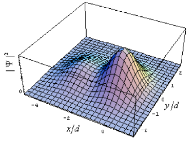
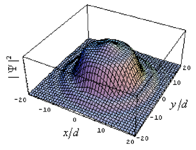
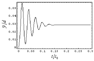
In Fig.1 and Fig.2 we represent the hole density for initial wave packet, Eq.(6) for $\gamma_{1}=7.65$ and $\gamma_{2}=2.41$, which correspond to $GaAs$, with width $d=3\cdot 10^{-6}cm$ and $k_{0}=2\cdot 10^{6}cm^{-1}$ at the moment $t=0.2$ (in units of $t_{0}=md^{2}/2\gamma_{2}\hbar$) (Fig.1); with width $d=3\cdot 10^{-6}cm$ and $k_{0}=0$ at the moment $t=4$ (in units of $t_{0}$) (Fig.2).

It is not difficult to see in Fig.1 and Fig.2 that the parameter $a=k_{0}d$ regulates the character of wave packet evolution. For the case $a>>1$ (see Fig.1) the initial wave packets split into two parts and their evolution is accompanied by the Zitterbewegung phenomenon. This dynamics is a result of interference of the hole states laying near the point $\vec{k}_{0}$ in momentum space. The splitting of the wave packets into two parts which propagate with unequal group velocity and have different angular momentum polarizations, appears due to the presence of the light and heavy holes states in the expansion the initial wave packet. As usual, the splitting is accompanied by the packet broadening which appears due to the effect of dispersion.

The ZB is a result of interference and a complex space-time evolution of two parts of wave packet. In another extreme case, when the inequality $a<<1$ takes place, the oscillations of the probability density at the circumference of the wave packet are closely related to the interference of heavy- and light-hole states located in vicinity of the point $\vec{k}=0$ in the momentum space (see Fig.2). This interference gives rise to the formation of the circular ripples around the packet center. The local period of these oscillations of probability density is not constant, it decreases with increasing radius of the ripple and time. This conclusion can be illustrated by the analytical expression for the density probabilities for $a=0$. For example, the analytical expression for the first component of wave function is

$$\halign{\hbox to\displaywidth{$\hfil\displaystyle#\hfil$}\cr 0.0pt{\hfil$\displaystyle|\Psi_{1}(\vec{r},t)|^{2}=\frac{1}{16\pi d^{2}}\Bigg{\{}\frac{9\exp(-\frac{r^{2}}{d^{2}(1+\omega_{L}^{2}t^{2})})}{1+\omega_{L}^{2}t^{2}}+\frac{\exp(-\frac{r^{2}}{d^{2}(1+\omega_{H}^{2}t^{2})})}{1+\omega_{H}^{2}t^{2}}\cr 0.0pt{\hfil$\displaystyle\hfill+6\frac{\exp(-\frac{r^{2}}{2d^{2}(1+\omega_{L}^{2}t^{2})}-\frac{r^{2}}{2d^{2}(1+\omega_{H}^{2}t^{2})})}{1+\omega_{L}^{2}\omega_{H}^{2}t^{4}+\omega_{L}^{2}t^{2}+\omega_{H}^{2}t^{2}}\Bigg{[}(1+\omega_{L}\omega_{H}t^{2})\times\hfill\cr 0.0pt{\hfil$\displaystyle\hfill\times\cos(\xi(t,r))+(\omega_{L}-\omega_{H})t\sin(\xi(t,r))\Bigg{]}\Bigg{\}},\hfill\cr}}}}$$

where $\omega_{L}=\hbar(-\gamma_{1}+2\gamma_{2})/d^{2}m$, $\omega_{H}=-\hbar(\gamma_{1}+2\gamma_{2})/d^{2}m$, $\Omega=\frac{\omega_{L}}{1+\omega_{L}^{2}t^{2}}+\frac{\omega_{H}}{1+\omega_{H}^{2}t^{2}}$, and $\xi(t,r)=\frac{r^{2}t}{2d^{2}}\Omega$. This expression contains oscillating terms which are proportional to functions $\cos(\xi(t,r))$ and $\sin(\xi(t,r))$, describing the ripples structure at Fig.2. It should be noted, however, that these oscillations do not provoke the ZB of average coordinate of packet center.

Figure 3: (Color online) The average coordinate $\bar{y}(t)$ of the packet center for different cases of value $a=k_{0}d$.

To analyze the motion of the packet center we have to find the average value of the position operator. To do it, let us use the momentum representation. The components $C_{\alpha}(\vec{k},t)$ ($\alpha=1,...4$) of wave function (5) in this representation can be obtained from Eqs.(4), (5), (6). After that the usual definition

$$\bar{x}_{i}(t)=\sum\limits_{\alpha=1}^{4}\int d\vec{k}C_{\alpha}^{\ast}(\vec{k},t)i\frac{d}{dk_{i}}C_{\alpha}(\vec{k},t),~{}~{}i=1,2$$

leads to

$$\bar{x}(t)=\frac{\hbar k_{0}}{m}(\gamma_{2}-\gamma_{1})t,$$

$$\bar{y}(t)=\frac{3}{4k_{0}}\Bigg{[}\exp(-\frac{(at/t_{0})^{2}}{1+(t/t_{0})^{2}})\cos(\frac{a^{2}t/t_{0}}{1+(t/t_{0})^{2}})-1\Bigg{]}.$$

We see that the center of wave packet moves along $x$ direction with constant velocity $\bar{V}_{0x}=\frac{\hbar k_{0}}{m}(\gamma_{2}-\gamma_{1})$. This expression also can be found from the equation

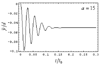
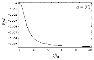
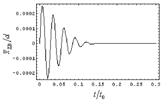
$$\bar{V}_{0x}=\frac{3}{4}V_{L}+\frac{1}{4}V_{H},$$

where $V_{L(H)}=\frac{1}{\hbar}\frac{\partial E_{L(H)}}{\partial k_{x}}|_{k_{x}=k_{0}}$ are the velocities of light (heavy) holes along $x$ axis at $k_{x}=k_{0}$ and $E_{L(H)}$ are determined by Eq.(2). The coefficients $3/4$ and $1/4$ correspond to relative parts of $L-$ and $H-$ holes. The motion of the wave packet center along $x$ is accompanied by the oscillations of the packet center at $a>1$ in a perpendicular direction or Zitterbewegung (Eq.(15)). It is easy to see that such trembling motion has a transient character as for other systems with two-band structures (Fig.3 for $a=15$). As it follows from Eqs.(14), (15) for a given initial polarization of the wave packet the ZB occurs in the direction perpendicular to the initial momentum $p_{0x}=\hbar k_{0}$. At large enough time $t>>t_{0}$ the packet center shifts in $y$ direction at the values of

$$y_{0}=\frac{3}{4k_{0}}({\rm e}^{-a^{2}}-1)$$

in accordance with Eq.(15). The Fig.3 for $a=0.1$ obviously demonstrates the monotonic behavior of $\bar{y}(t)$.

ii) As a second example we compute the free space-time evolution of the Gaussian packet

$$\Psi(\vec{r},0)=\frac{\exp(-\frac{r^{2}}{2d^{2}}+ik_{0}x)}{d\sqrt{2\pi}}\pmatrix{1\cr 0\cr 1\cr 0}.$$

This expression is obtained as a superposition of two components, corresponding to the light and heavy holes. It should be mentioned that the relative weight of the light and heavy holes is not constant in momentum space in contrast to the previous case, Eq.(6). Really, as it follows from Eqs.(5), (17) the amplitudes $C_{L(H),i}$ are

$$\halign{\hbox to\displaywidth{$\hfil\displaystyle#\hfil$}\cr 0.0pt{\hfil$\displaystyle C_{L1}=C_{H1}=0,~{}~{}~{}C_{L2}=\frac{\sqrt{2}}{4}f_{\vec{k}}(\sqrt{3}{\rm e}^{i2\varphi}+1),\cr 0.0pt{\hfil$\displaystyle\hfill C_{H2}=\frac{\sqrt{2}}{4}f_{\vec{k}}({\rm e}^{i2\varphi}-\sqrt{3}).\hfill\hbox to0.0pt{\hss(}18)\cr}}}$$

Substituting Eq.(18) into Eq.(5) we obtain the components of wave function

$$\Psi_{2}(\vec{r},t)=\Psi_{4}(\vec{r},t)=0,$$

$$\halign{\hbox to\displaywidth{$\hfil\displaystyle#\hfil$}\cr 0.0pt{\hfil$\displaystyle\Psi_{1}(\vec{r},t)=\frac{\sqrt{2}}{8}\frac{d}{\sqrt{\pi}}{\rm e}^{-a^{2}/2}\Bigg{(}\frac{3{\rm e}^{\beta/2\delta_{L}}}{\delta_{L}}+\frac{{\rm e}^{\beta/2\delta_{H}}}{\delta_{H}}\Bigg{)}+\hfill\cr 0.0pt{\hfil$\displaystyle+\frac{\sqrt{3}d{\rm e}^{-a^{2}/2}}{4\sqrt{2\pi}}\frac{a^{2}d^{2}+(x-iy)^{2}}{(ad-y)^{2}+x^{2}}\Bigg{(}\frac{{\rm e}^{\beta/2\delta_{L}}}{\delta_{L}}(1-~{}~{}~{}~{}\cr 0.0pt{\hfil$\displaystyle\hfill-\frac{2\delta_{L}}{\beta})-\frac{{\rm e}^{\beta/2\delta_{H}}}{\delta_{H}}(1-\frac{2\delta_{H}}{\beta})\Bigg{)},\hfill\hbox to0.0pt{\hss(}19)\cr}}}}$$

$$\halign{\hbox to\displaywidth{$\hfil\displaystyle#\hfil$}\cr 0.0pt{\hfil$\displaystyle\Psi_{3}(\vec{r},t)=\frac{\sqrt{2}}{8}\frac{d}{\sqrt{\pi}}{\rm e}^{-a^{2}/2}\Bigg{(}\frac{{\rm e}^{\beta/2\delta_{L}}}{\delta_{L}}+\frac{{3\rm e}^{\beta/2\delta_{H}}}{\delta_{H}}\Bigg{)}+\hfill\cr 0.0pt{\hfil$\displaystyle+\frac{\sqrt{3}d{\rm e}^{-a^{2}/2}}{4\sqrt{2\pi}}\frac{a^{2}d^{2}+(x+iy)^{2}}{(ad+y)^{2}+x^{2}}\Bigg{(}\frac{{\rm e}^{\beta/2\delta_{L}}}{\delta_{L}}(1-~{}~{}~{}~{}\cr 0.0pt{\hfil$\displaystyle\hfill-\frac{2\delta_{L}}{\beta})-\frac{{\rm e}^{\beta/2\delta_{H}}}{\delta_{H}}(1-\frac{2\delta_{H}}{\beta})\Bigg{)},\hfill\hbox to0.0pt{\hss(}20)\cr}}}}$$

where $\delta_{L}$, $\delta_{H}$ and $\beta$ are determined by Eq.(12). The results of the calculation of average values of $x$ and $y$ for this polarization are

$$\bar{x}(t)=V_{0x}t+x_{ZB}(t),$$

where the constant velocity is defined by the expression

$$V_{0x}=\frac{\hbar k_{0}}{m}\Bigg{[}-\gamma_{1}+\gamma_{2}\sqrt{3}\Bigg{(}1-\frac{1}{a^{2}}+\frac{1}{a^{4}}-\frac{{\rm e}^{-a^{2}}}{a^{4}}\Bigg{)}\Bigg{]},$$

and $x_{ZB}(t)$ describes the oscillatory motion (Zittebewegung)

$$\halign{\hbox to\displaywidth{$\hfil\displaystyle#\hfil$}\cr 0.0pt{\hfil$\displaystyle\bar{x}_{ZB}(t)=\frac{\sqrt{3}}{2k_{0}a^{2}}\exp(-\frac{a^{2}t^{2}/t_{0}^{2}}{1+t^{2}/t_{0}^{2}})\Bigg{(}\sin(\frac{a^{2}t/t_{0}}{1+t^{2}/t_{0}^{2}})-\frac{t}{t_{0}}\times~{}~{}~{}~{}\cr 0.0pt{\hfil$\displaystyle\hfill\times\cos(\frac{a^{2}t/t_{0}}{1+t^{2}/t_{0}^{2}})\Bigg{)}+\frac{\sqrt{3}}{2k_{0}a^{2}}{\rm e}^{-a^{2}}\frac{t}{t_{0}},\hfill\hbox to0.0pt{\hss(}23)\cr}}}$$

$$\halign{\hbox to\displaywidth{$\hfil\displaystyle#\hfil$}\cr 0.0pt{\hfil$\displaystyle\bar{y}(t)=\frac{\sqrt{3}}{4k_{0}}\Bigg{[}1-\frac{1}{a^{2}}-(1-\frac{1}{a^{2}})\exp(-\frac{a^{2}t^{2}/t_{0}^{2}}{1+t^{2}/t_{0}^{2}})\cos(\frac{a^{2}t/t_{0}}{1+t^{2}/t_{0}^{2}})+\cr 0.0pt{\hfil$\displaystyle\hfill+\frac{t}{a^{2}t_{0}}\exp(-\frac{a^{2}t^{2}/t_{0}^{2}}{1+t^{2}/t_{0}^{2}})\sin(\frac{a^{2}t/t_{0}}{1+t^{2}/t_{0}^{2}})\Bigg{]}.\hfill\hbox to0.0pt{\hss(}24)\cr}}}$$

The space-time diagram of this solution, shown in Fig.4 again shows the Zitterbewegung of the position’s mean values. It is interesting to stress that for the packet polarization determined by Eq.(17) the oscillatory behavior occurs in both $x$ and $y$ directions. The amplitude of oscillations in $x$ direction is much less than that in $y$ direction.

Figure 4: (Color online) The space-time diagram of the packet center for the initial wave packet, Eq. (17) with $a=15$.

As it follows from Eqs.(15), (23), (24) the character of trembling motion strongly depends on the parameter $a=k_{0}d$ as for the other system.DMF ; MDF Really, it is easy to see that oscillations of ${\bar{\vec{r}}}(t)$ (which are connected with the terms $\cos(\frac{a^{2}t/t_{0}}{1+t^{2}/t_{0}^{2}})$ or $\sin(\frac{a^{2}t/t_{0}}{1+t^{2}/t_{0}^{2}})$) occur if $a^{2}\geq\pi$. However the value $a$ should not be too large since the amplitude of oscillations ($\sim\exp(-\frac{a^{2}t^{2}/t_{0}^{2}}{1+t^{2}/t_{0}^{2}})$) decreases rapidly when $a$ increase.

Notice also that if we consider the plane wave that corresponds to $d\rightarrow\infty$ (i.e. $a\rightarrow\infty$ and $t_{0}\rightarrow\infty$) then we obtain from Eqs.(14), (15)

$$\halign{\hbox to\displaywidth{$\hfil\displaystyle#\hfil$}\cr 0.0pt{\hfil$\displaystyle\bar{x}(t)=\frac{\hbar k_{0}}{m}(\gamma_{2}-\gamma_{1})t,\cr 0.0pt{\hfil$\displaystyle\hfill\bar{y}(t)=\frac{3}{4k_{0}}\Bigg{(}\cos(\frac{2\gamma_{2}\hbar k_{0}^{2}t}{m})-1\Bigg{)},\hfill\hbox to0.0pt{\hss(}25)\cr}}}$$

and correspondingly for the second polarization (Eq.(17))

$$\halign{\hbox to\displaywidth{$\hfil\displaystyle#\hfil$}\cr 0.0pt{\hfil$\displaystyle\bar{x}(t)=\frac{\hbar k_{0}}{m}(\sqrt{3}\gamma_{2}-\gamma_{1})t,\cr 0.0pt{\hfil$\displaystyle\hfill\bar{y}(t)=\frac{\sqrt{3}}{4k_{0}}\Bigg{(}1-\cos(\frac{2\gamma_{2}\hbar k_{0}^{2}t}{m})\Bigg{)}.\hfill\hbox to0.0pt{\hss(}26)\cr}}}$$

iii) Let us consider now the third example when the initial wave packet has the following form:

$$\Psi(\vec{r},0)=\frac{\exp(-\frac{r^{2}}{2d^{2}}+ik_{0}x)}{d\sqrt{2\pi}}\pmatrix{1\cr i\cr 0\cr 0}.$$

Using expression (5) and specifying the coefficients $C_{L(H),i}(\vec{k})$, we find the components of the wave function at arbitrary time:

$$\Psi_{1}(\vec{r},t)=\frac{d{\rm e}^{-a^{2}/2}}{4\sqrt{2\pi}}\Bigg{[}\frac{3{\rm e}^{\beta/2\delta_{L}}}{\delta_{L}}+\frac{{\rm e}^{\beta/2\delta_{H}}}{\delta_{H}}\Bigg{]},$$

$$\Psi_{2}(\vec{r},t)=i\frac{d{\rm e}^{-a^{2}/2}}{4\sqrt{2\pi}}\Bigg{[}\frac{{\rm e}^{\beta/2\delta_{L}}}{\delta_{L}}+\frac{3{\rm e}^{\beta/2\delta_{H}}}{\delta_{H}}\Bigg{]},$$

$$\halign{\hbox to\displaywidth{$\hfil\displaystyle#\hfil$}\cr 0.0pt{\hfil$\displaystyle\Psi_{3}(\vec{r},t)=\frac{\sqrt{3}d}{4\sqrt{2\pi}}{\rm e}^{-a^{2}/2}\frac{a^{2}d^{2}+(x+iy)^{2}}{(a^{2}d+y)^{2}+x^{2}}\times\cr 0.0pt{\hfil$\displaystyle\hfill\times\Bigg{[}\frac{{\rm e}^{\beta/2\delta_{L}}}{\delta_{L}}(1-\frac{2\delta_{L}}{\beta})-\frac{{\rm e}^{\beta/2\delta_{H}}}{\delta_{H}}(1-\frac{2\delta_{H}}{\beta})\Bigg{]},\hfill\hbox to0.0pt{\hss(30)}\cr}}}$$

$$\Psi_{4}(\vec{r},t)=i\Psi_{3}(\vec{r},t)$$

It is easy to see that for this polarization the time dependence of the full probability density is similar to the evolution in the case i) in sprite of that here all four components of wave function are not equal to zero. Here we note only that the average coordinate $\bar{x}(t)=-\frac{\hbar k_{0}\gamma_{1}}{m}t$, and $\bar{y}(t)$ has the same form as in the case i), Eq.(15). But as we will see below the spin density and average spin evolution in this case differ qualitatively from those in cases i) and ii).

III Alternating spin - 3/2 polarization

As was shown firstly in Ref.[19], the spin dynamics of spin - 3/2 hole is qualitatively different from those of spin - 1/2 electron systems. In contrast to spin - 1/2 electron systems, neither the magnitude nor the orientation of the angular momentum $\bar{\vec{S}}$ are conserved. In spite of the fact that the coupling of spin and orbital degrees of freedom cannot be written in terms of external or effective magnetic field, the hole spin polarization, as well as the higher-order multipoles demonstrate nontrivial dynamics in time and can precess due to the interference of heavy- and light- hole statesCulWin . In the Ref. [19] the main results concerning the alternating spin polarization in spin - 3/2 hole systems were obtained only for the initial states represented by the plane waves. Below we describe and visualize the spin dynamics of hole wave packets with different initial polarizations. For this purpose we consider the time evolution of components of the effective spin density $S_{i}(\vec{r},t)$ and their average values $\bar{S_{i}}(t)$

$$S_{i}(\vec{r},t)=\Psi^{+}(\vec{r},t)\hat{S}_{i}\Psi(\vec{r},t),$$

$$\bar{S}_{i}(\vec{r},t)=\int\Psi^{+}(\vec{r},t)\hat{S}_{i}\Psi(\vec{r},t)d\vec{r},$$

where $\Psi(\vec{r},t)$ is a four-component wave function and $\Psi^{+}(\vec{r},t)$ denotes the Hermitian conjugated wave function.

Firstly, we consider the wave packet, corresponding to the hole spin oriented initially along $z$ direction: $S_{z}=\frac{3}{2}$, Eq.(6). In this case it is easy to see that spin densities are equal to $S_{x}(\vec{r},t)=S_{y}(\vec{r},t)=0$, $S_{z}(\vec{r},t)=\frac{3}{2}|\Psi_{1}(\vec{r},t)|^{2}-\frac{1}{2}|\Psi_{3}(\vec{r},t)|^{2}$, where the components of wave function $\Psi_{1}(\vec{r},t)$ and $\Psi_{3}(\vec{r},t)$ are determined by Eqs.(9)-(11).

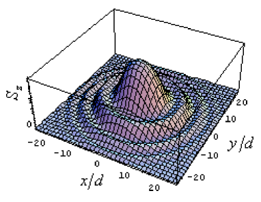
To illustrate the evolution of the hole spin density $S_{z}(\vec{r},t)$ we plot this function in Fig.5 for the moment of the time $t=15$ (in units of $t_{0}$) and for wave packet parameters $d=10^{-6}$ $cm$ and $k_{0}=10^{5}$ $cm^{-1}$. Just as for hole probability density the space-time evolution of the spin density strongly depends on the parameter $a$. In particular, for small values of $a$ as was demonstrated in Sec.II the splitting of wave packet is absent and oscillations of the probability density (ripples) arises on its periphery. Similar behavior of spin density $S_{z}(\vec{r},t)$ for $a=0.1$ one can observe in Fig.5.

Using Eq.(33) it is not difficult to find the average value $\bar{S}_{z}(t)$ for given initial polarization

$$\halign{\hbox to\displaywidth{$\hfil\displaystyle#\hfil$}\cr 0.0pt{\hfil$\displaystyle\bar{S_{z}}(t)=\frac{3}{4}\Bigg{[}1+\frac{\exp(-\frac{a^{2}(t/t_{0})^{2}}{1+(t/t_{0})^{2}})}{1+(t/t_{0})^{2}}\times\cr 0.0pt{\hfil$\displaystyle\hfill\times\Bigg{(}\cos(\frac{a^{2}t/t_{0}}{1+(t/t_{0})^{2}})-\frac{t}{t_{0}}\sin(\frac{a^{2}t/t_{0}}{1+(t/t_{0})^{2}})\Bigg{)}\Bigg{]}.\hfill\hbox to0.0pt{\hss(34)}\cr}}}$$

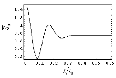
This expression obviously demonstrates that $\bar{S}_{z}(t)$ experiences the transient oscillations for the parameter $a>>1$ (see Fig.6). For $t/t_{0}>>1$ $\bar{S}_{z}(t)$ streams to the constant values 3/4. Note that the length of spin vector in this case is not constant. As it follows from Eq.(34) in the limiting case $d\rightarrow\infty$, i.e. for the plane wave, $\bar{S}_{z}$ is

$$\bar{S}_{z}(t)=\frac{3}{2}\cos^{2}\frac{2\gamma_{2}\hbar k_{0}^{2}t}{m}.$$

This result coincides with that in Ref.[19].

Figure 5: (Color online) The angular momentum density $S_{z}(\vec{r},t)$ for initial wave packet, Eq.(6) with $k_{0}=10^{5}~{}cm^{-1}$, $d=10^{-6}~{}cm$, $a=0.1$ at t=15 (in units of $t_{0}$).

Figure 6: (Color online) The average value of angular momentum $\bar{S}_{z}(t)$ for initial spinor, Eq.(6) for $a=6$.

For the second example presented in Sec.II, Eq.(17), the initial values of effective spin are $\bar{S}_{x}(0)=\bar{S}_{y}(0)$, $\bar{S}_{z}(0)=1/2$, and space-time evolution of spin density components $S_{i}(\vec{r},t)$ are similar to that discussed above. Note that for these two cases the initial vector $\bar{\vec{S}}(0)$ is perpendicular to the average momentum $\bar{\vec{p}}_{0}=(\hbar k_{0},0,0)$. But as was revealed in Ref.[19], the most interesting spin dynamics characterized by hole spin precession occurs when $\vec{\rho}(0)$ is not perpendicular or parallel to $\bar{\vec{p}}_{0}$.

Such initial condition is realized in particular for the wave packet given by Eq.(27). Using the expressions for the components of the wave function at arbitrary time Eqs.(28), (29), (30), (31) one can obtain the hole spin density $\vec{S}(\vec{r},t)$ and the components of average spin $\bar{\vec{S}}(t)$

$$\halign{\hbox to\displaywidth{$\hfil\displaystyle#\hfil$}\cr 0.0pt{\hfil$\displaystyle\bar{S_{x}}(t)=-\frac{\sqrt{3}}{2}+\frac{\sqrt{3}}{8a^{2}}\Bigg{[}1-\exp(-\frac{a^{2}(t/t_{0})^{2}}{1+(t/t_{0})^{2}})\times\cr 0.0pt{\hfil$\displaystyle\hfill\times\cos(\frac{a^{2}t/t_{0}}{1+(t/t_{0})^{2}})\Bigg{]}.\hfill\hbox to0.0pt{\hss(36)}\cr}}}$$

$$\halign{\hbox to\displaywidth{$\hfil\displaystyle#\hfil$}\cr 0.0pt{\hfil$\displaystyle\bar{S_{y}}(t)=-\frac{\sqrt{3}}{2}\frac{\exp(-\frac{a^{2}(t/t_{0})^{2}}{1+(t/t_{0})^{2}})}{1+(t/t_{0})^{2}}\Bigg{(}\sin(\frac{a^{2}t/t_{0}}{1+(t/t_{0})^{2}})+\cr 0.0pt{\hfil$\displaystyle\hfill+\frac{t}{t_{0}}\cos(\frac{a^{2}t/t_{0}}{1+(t/t_{0})^{2}})\Bigg{)}+\frac{\sqrt{3}}{4a^{2}}\exp(-\frac{a^{2}(t/t_{0})^{2}}{1+(t/t_{0})^{2}})\times\cr 0.0pt{\hfil$\displaystyle\hfill\times\sin(\frac{a^{2}t/t_{0}}{1+(t/t_{0})^{2}}).\hfill\hbox to0.0pt{\hss(37)}\cr}}}}$$

$$\halign{\hbox to\displaywidth{$\hfil\displaystyle#\hfil$}\cr 0.0pt{\hfil$\displaystyle\bar{S_{z}}(t)=\frac{1}{4}\Bigg{[}1+\frac{3\exp(-\frac{a^{2}(t/t_{0})^{2}}{1+(t/t_{0})^{2}})}{1+(t/t_{0})^{2}}\times\cr 0.0pt{\hfil$\displaystyle\hfill\times\Bigg{(}\cos(\frac{a^{2}t/t_{0}}{1+(t/t_{0})^{2}})-\frac{t}{t_{0}}\sin(\frac{a^{2}t/t_{0}}{1+(t/t_{0})^{2}})\Bigg{)}\Bigg{]}.\hfill\hbox to0.0pt{\hss(38)}\cr}}}$$

These expressions become more simple in the limit case $d\rightarrow\infty$, i.e. for the plain wave propagating along the $x$ axis with wave vector $k_{0}$

$$\bar{S}_{x}(t)=-\frac{\sqrt{3}}{2},~{}~{}~{}~{}\bar{S}_{y}(t)=-\frac{\sqrt{3}}{2}\sin\frac{2\gamma_{2}\hbar k_{0}^{2}t}{m},$$

$$\bar{S}_{z}(t)=\frac{1}{4}\Bigg{(}1+3\cos(\frac{2\gamma_{2}\hbar k_{0}^{2}t}{m})\Bigg{)}.$$

Last formulas clearly demonstrate the precession of vector $\bar{\vec{S}}(t)$ about the wave vector $\vec{k}_{0}$: the end of vector $\bar{\vec{S}}(t)$ describes ellipsis on the plane $(S_{y},S_{z})$

$$\frac{(\bar{S}_{y}(t))^{2}}{m^{2}}+\frac{(\bar{S}_{z}-1/4)^{2}}{n^{2}}=1,$$

where $m=\sqrt{3}/2$, $n=3/4$.

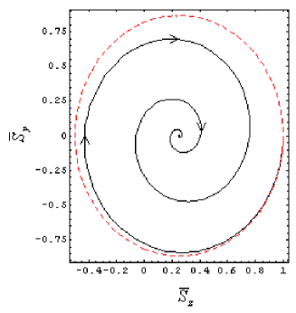
In our case for the wave packet of finite width the time evolution of the effective spin becomes more complicated as it follows from Eqs.(36)-(38). Firstly, the component $\bar{S}_{x}(t)$ depends on time, although this dependence is weak enough both for $a>>1$ and $a<<1$. Secondly, the ”precession” in $(S_{y},S_{z})$ plane acquires the transient character which is demonstrated in Fig.7. As one can see from Fig.7 the component $\bar{S}_{y}(0)=\bar{S}_{y}(\infty)=0$ and the component $\bar{S}_{z}$ changes its values from $\bar{S}_{z}(0)=1$ to $\bar{S}_{z}(\infty)=1/4$.

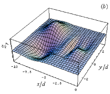
To illustrate the spin density we plot the components $S_{z}(\vec{r},t)$ and $S_{y}(\vec{r},t)$ in Fig.8 for the moments of the time $t=0.1$ and $t=0.5$ (in units of $t_{0}$) correspondingly and for $a=6$. The Fig. 8(b) demonstrates clearly the splitting of the angular momentum density into two parts similar to probability density discussed in Sec.II for $a>>1$. The angular momentum density changes its sign within each part that looks like as multipole structure.

Figure 7: (Color online) The transient precession of average angular moment vector $\bar{\vec{S}}(t)$ (in plane $(S_{y},S_{z})$) about the vector $\vec{k}_{0}~{}||~{}Ox$ for wave packet described by Eq.(27) ($a=10$). Dashed line in accordance with Eq.(40) corresponds to the hole spin precession for the plane wave.

Figure 8: (Color online) The angular momentum density $S_{z}(\vec{r},t)$ and $S_{y}(\vec{r},t)$ for initial wave packet, Eq.(27) for $k_{0}=2\cdot 10^{6}~{}cm^{-1}$, $d=3\cdot 10^{-6}~{}cm$, $a=6$ at $t=0.1$ (a) and $t=0.5$ (b) (in units of $t_{0}$).

IV Conclusion

Using the Luttinger isotropic model we have studied the dynamics of wave packets in hole 3/2 effective spin systems. The analytical expressions for the four component wave function are obtained and the probability densities as well as the effective spin densities are visualized for different initial spin polarizations. Two different types of the spatial evolution of wave packets are found. In the case when the parameter $a>>1$ the initially localized packet splits into two parts propagating with different group velocities and having various effective spin polarizations. Similarly to the wave packet evolution in systems with spin-orbit couplingDMF this evolution is accompanied by the oscillations of packet center or Zitterbewegung. These oscillations quickly fade away when the distance between two parts of split packet exceeds its initial value. Another scenario of the evolution is realized for a small value of parameter $a$, namely when $a<<1$. In this case the probability density remains almost axial symmetric with time, but the ripples appear at the circumference of the density distribution. These ripples arise owing to the interference of heavy- and light-hole states located in the vicinity of the point $\vec{k}=0$ in momentum space. It should be noted that this interference does not stimulate the oscillations of packet center $\bar{\vec{r}}(t)$ or ZB.

It is known that the spin dynamics of the holes, described by an effective spin - 3/2, differs qualitatively from that for spin - 1/2 electrons. The main and striking peculiarity of hole spin dynamics is the nontrivial periodic motion of average spin vector in spin space, which can be viewed as a precession. We have studied in detail such unusual behavior for the hole wave packets. We have shown that finite width of wave packet is responsible for the transient character of spin precession. The analytical and numerical study of the influence of $a$ parameter on the angular momentum density and average spin vector is presented. For the case when $a>>1$ the density of angular momentum splits into two parts having multipole polarization, but for $a<<1$ the angular momentum density preserves almost the initial cylindrical symmetry.

The experimental observation of trembling motion of $\vec{r}(t)$ and spin precession in crystalline solids is a long standing problem of condensed matter physics. The possible methods of producing of electron and hole wave packets as well as the observation of ZB effects was analyzed in numerous of recent publications. As was discussed in Ref. [20], the hole packets can be excited optically in nondegenerate 3D hole gas by using a polarized laser beam. If laser beam has a finite size the optically exited wave packet will consist of states of light and heavy holes lying in the range of $d^{-1}$ in vicinity of the point $\vec{k}=0$ and can have a definite spin polarization. To obtain the wishful average momentum $k_{0}$ the electric field pulse with duration of some picosecond can be applied after excitation. During the process of optical excitation electrons will excited also, but the electric field will separate positive and negative charges. The ZB evolution to be robust against disorder provided $\omega_{ZB}>1/\tau_{s}$ and $\omega_{ZB}>1/\tau_{p}$ where $\tau_{s}$ and $\tau_{p}$ are spin and momentum relaxation times correspondingly. As was verified experimentally (e.g. in $GaAs$ and $InAs$ $\tau_{S}$ is of the order $10-100$ ps) these conditions can be fulfilled in clear semiconductors.

An interesting method of observation of trembling motion of charged particles in solids was proposed by Rusin and Zavadski in Ref. [15]. They note that the typical period of ZB oscillation is comparable with the period of Bloch oscillations, and so the method which early was used for observation of Bloch oscillation in superlatticies at the presence of electric fieldLyssenko can be used also for the ZB observation. The results of Sec. II and Sec. III of this work show that this method can be used also for ZB observation in Luttinger spin - 3/2 system.

The information about the evolution of hole wave packets is important in the context of application for analysis of functioning of different spintronic devices (e.g. Datta - Das hole spin effect transistorPala ) and for understanding the transport phenomena and spin related dynamics.

References

• (1) E. Schrödinger, Sitzungsber. Peuss. Akad. Wiss. Phys. Math.KI. 24, 418 (1930). See also A.O. Barut and A.J. Bracken, Phys. Rev. D 23, 2454 (1981).
• (2) J. A.  Lock, Am. J. Phys. 47, 797 (1979).
• (3) I. Ferrari and G. Russo, Phys. Rev. B 42, 7454 (1990).
• (4) F. Cannata, I. Ferrari and G. Russo Solid State Commun. 74, 309 (1990).
• (5) S. W. Vonsovsky, M. S. Svirsky, and L. M. Svirskaya, Theor. Mathem. Fizika, 94, 343 (1993) (in Russian).
• (6) W. Zawadski, Phys. Rev. B 72, 085217 (2005).
• (7) W. Zawadski, Phys. Rev. B 74, 205439 (2006).
• (8) J. Schlieman, D. Loss and R. M. Westervelt, Phys. Rev. Lett. 94, 206801 (2006).
• (9) V. Ya. Demikhovskii, G. M. Maksimova, and E. V. Frolova, Phys.Rev. B 78, 115401 (2008).
• (10) M. Katsnelson, Eur. Phys. J. B 51, 157(2007).
• (11) G. M. Maksimova, V. Ya. Demikhovskii, and E. V. Frolova, Phys.Rev. B 78, 235321 (2008).
• (12) D. Lurie and S. Cremer, Physica (Amsterdam) 50, 224 (1970).
• (13) Xiangdong Zhang, Phys. Rev. Lett., 100, 113903 (2008).
• (14) N. M. Rusin and W. Zawadski , J.Phys. Condence. Matter, 19, 136219 (2007).
• (15) N. M. Rusin and W. Zawadski, arXiv: cond-mat/0909.0463v1 (2009) (unpublished).
• (16) Z. F. Jiang, R. D. Li, S.-C. Zhang, and W. M. Liu, Phys. Rev. B 72, 045201(2005).
• (17) J. Cserti and G. David, Phys. Rev. B 74, 172305(2006); G. David and J. Cserti, arXiv: cond-mat/0909.2004v1 (2009) (unpublished).
• (18) R. Winkler, U. Zulicke, and J. Bolte, Phys. Rev. B 75, 205314(2007).
• (19) D. Culcer, C. Lechner, and R. Winkler, Phys. Rev. Lett. 97, 106601(2006)
• (20) D. Culcer, Y. Yao, Q. Niu, Phys. Rev. B 72, 085110(2005).
• (21) J. M. Luttinger, Phys. Rev. B 102, 1030 (1956).
• (22) N. O. Lipari and A. Baldereschi, Phys. Rev. Lett. 25, 1660 (1970).
• (23) V. G. Lyssenko et al., Phys. Rev. Lett. 79, 301 (1997).
• (24) M. G. Pala, M. Governale, J. Konig, U. Zulicke, and G. Iannaccone, Phys. Rev. B 69, 045304 (2004).