The Shape of the Primordial Power Spectrum: A Last Stand Before Planck

Abstract

We present a minimally-parametric reconstruction of the primordial power spectrum using the most recent cosmic microwave background and large scale structure data sets. Our goal is to constrain the shape of the power spectrum while simultaneously avoiding strong theoretical priors and over-fitting of the data. We find no evidence for any departure from a power law spectral index. We also find that an exact scale-invariant power spectrum is disfavored by the data, but this conclusion is weaker than the corresponding result assuming a theoretically-motivated power law spectral index prior. The reconstruction shows that better data are crucial to justify the adoption of such a strong theoretical prior observationally. These results can be used to determine the robustness of our present knowledge when compared with forthcoming precision data from Planck.

I Introduction

The deviation from scale invariance of the primordial scalar power spectrum is a critical prediction of inflation, and unlike other potential signatures such tensor modes or non-Gaussianity, it is the only signature that is generic to all inflationary models. It is therefore a vital test of the inflationary paradigm, and we address it with a minimally parametric approach.

Briefly, the idea is as follows. Choose a functional form which allows a great deal of freedom in the form of the deviation from scale invariance (e.g. smoothing splines). Naively fitting this to the data will lead one to fit the fluctuations due to cosmic variance and experimental noise, with arbitrary improvement in the chi-square. Instead, one performs cross-validation: throw out some of the data (the validation set), fit the rest (the training set), and see how well it predicts the validation set. A very good fit to the training set, which poorly predicts the validation set, indicates over-fitting of noisy data. The final ingredient in the algorithm is a roughness penalty, a parameter that penalizes a high degree of structure in the functional form. By performing cross-validation as a function of this penalty, one can judge when the amount of freedom in the smoothing spline is what the data require without fitting the noise. A minimally parametric power spectrum reconstruction combined with a roughness penalty set by cross-validation thus provides a method of determining smooth departures from scale invariance which avoids two pitfalls. Firstly, a strong theory prior on the form of the power spectrum (e.g. the commonly used power law prescription) can lead to artificially tight constraints on – even a spurious detection of – a deviation from scale invariance, which is mostly due to the strength of the prior than that of the data. Secondly, simple binning techniques Bridle et al. (2003); Spergel et al. (2007); Hannestad (2004); Bridges et al. (2006, 2007) or direct inversion Shafieloo and Souradeep (2004, 2008); Kogo et al. (2004); Tocchini-Valentini et al. (2006, 2005); Nagata and Yokoyama (2008, 2009); Ichiki and Nagata (2009); Nicholson and Contaldi (2009); Nicholson et al. (2009) of the data to obtain the primordial power spectrum can lead one to fit noisy data with a large improvement in chi-square. A minimally parametric approach combined with cross-validation avoids these issues, providing a way to actually determine the strength of the shape prior justified by the quality of the data. Cross-validation would also be helpful for alternative minimally-parametric methods Mukherjee and Wang (2005); Leach (2006) e.g. in choosing the number of basis functions.

In this work, we use the best available data over a wide range of scales corresponding to the longest “lever arm” of wavenumbers currently extant, to reconstruct the shape of the primordial power spectrum in a minimally-parametric way. ESA’s Planck satellite, which has already begun taking data, is expected to provide superior constraints The Planck Collaboration (2006) on the shape of the primordial scalar power spectrum by 2012. Our goal here is to establish a benchmark of what was known about the shape of the power spectrum before the Planck analysis.

Figure 1: (Left) WMAP 5 year data Nolta et al. (2009) and (right) external CMB data from ACBAR and QUaD Reichardt et al. (2009); Brown et al. (2009), showing knot placement (triangles, arbitrary normalization) and the cross-validation set-up. CV_A is red and CV_B is blue. We show only the temperature data here (in $\mu$K²) as the constraints on the power spectrum shape come mostly from the temperature data; in practice for each data set we also use the polarization data, which is crucial in lifting degeneracies with the cosmological parameters. The light blue line is a concordance LCDM model.

II Methodology

We perform a minimally-parametric reconstruction of the primordial power spectrum based on the method of Ref. Sealfon et al. (2005). Since the simplest inflationary models, which are consistent with the data, predict the primordial power spectrum to be a smooth function, we search for smooth deviations from scale invariance with a cubic smoothing spline technique (for details, see Refs. Green and Silverman (1994); Sealfon et al. (2005); Verde and Peiris (2008) which we only briefly summarize here). In this approach, one aims to recover a function $f(x)$ from measurements $\hat{f}$ at $n$ discrete points $x_{i}$.

Consider a description of $f$ by a piecewise cubic spline $F(x)$. It is uniquely defined by the values of $F$ at $N$ “knots” once we ask for continuity of $F(x)$ and its first and second derivatives at the knots, and two boundary conditions: we require the second derivative to vanish at the exterior knots. In our application, $F(x)$ is the primordial power spectrum $P(k)$, and the data are: the angular power spectrum of the 5 year Wilkinson Microwave Anisotropy Probe (WMAP5) cosmic microwave background (CMB) temperature and polarization Nolta et al. (2009); alone or in combination with higher resolution, ground-based CMB experiments (QUaD Brown et al. (2009) and ACBAR Reichardt et al. (2009)); or with large scale structure data: the Sloan Digital Sky Survey (SDSS) Data Release 7 (DR7) Luminous Red Galaxy (LRG) power spectrum Reid et al. (2009); and the Lyman-alpha forest (Ly$\alpha$) power spectrum constraints from Ref. McDonald et al. (2006). This work thus represents a significant advance over previous work Verde and Peiris (2008), with a new WMAP release (two further years of data and a significant advance in the understanding of systematic errors) plus substantial improvements in both ground-based CMB data and large-scale structure data.

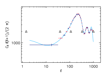
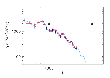
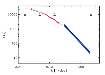
We use 5 to 7 knots depending on the data set considered (see Table 1 for details; the locations of the knots in $k$ space are indicated in Figs. 1 and 2). If the knot values were allowed infinite freedom and were set simply by minimizing the chi-square, in general the reconstruction would fit features created by the random noise present in the data. It is therefore necessary to add a roughness penalty which we chose to be the integral of the second derivative of the spline function. The roughness penalty is weighted by a smoothing parameter: by increasing the smoothing parameter the roughness penalty effectively reduces the degrees of freedom, disfavouring jagged functions that “fit the noise”.

Table 1: The cross-validation set-up and the adopted number of knots for each data set used in the analysis.

DATA SET	CVA	CVB	# knots
WMAP5	yes	yes	$5$
QUaD	no	yes	$6$
ACBAR	yes	no	$6$
SDSS DR7	yes	no	$6$
Ly$\alpha$	no	yes	$7$

In generic applications of smoothing splines, cross-validation is a rigorous statistical technique for choosing the optimal smoothing parameter. Cross-validation (CV) quantifies the notion that if the underlying function has been correctly recovered, it should accurately predict new, independent data. To make the problem computationally manageable, we opt for a $n/2$–fold cross-validation, where $n$ is the number of data points. That is, the data set is split into two halves, say, $A$ and $B$. A Markov chain Monte Carlo (MCMC) parameter estimation analysis (for a given smoothing parameter) is carried out on one half of the data, finding the best fit model. Then the log likelihood of the second half of the data given the best fit model for the first half, CV_AB, is computed and stored. This is repeated by switching the roles of the two halves, obtaining CV_BA. The sum, CV_AB+CV_BA, gives the “CV score” for that smoothing parameter. Finally, the smoothing parameter that best describes the entire data set is the one that minimizes the CV score. Table 1 gives details of the implementation. Note that, as in Ref. Verde and Peiris (2008), the basic cosmological parameters ($\omega_{b}h^{2}$, $\Omega_{c}h^{2}$, $\Theta_{A}$, $\tau$) are varied in the MCMC as well as the values of the smoothing spline at the knots, which describe the primordial power spectrum. The MCMC is implemented with modified versions of the CAMB Lewis et al. (2000) and COSMOMC Lewis and Bridle (2002) packages, with very stringent convergence criteria. Now we will describe our treatment of the data.

Figure 2: Large-scale structure power spectrum in units of ($h$/Mpc)³, showing knot placement (triangles, arbitrary normalization) and cross-validation set-up. CV_A is red and CV_B is blue. Red points represent the LRG power spectrum from Ref. Reid et al. (2009). The Lyman alpha measurement is represented by a filled box encompassing the constraints on the observed flux power spectrum from Ref. McDonald et al. (2006). The light blue line is a concordance LCDM model.

CMB Data: We use the $v3p2$ version of the WMAP5 likelihood function with standard options, with the temperature data divided into alternate (roughly equal signal-to-noise) $\ell$ bins for CV_A and CV_B respectively, exactly as in Ref. Verde and Peiris (2008). The polarization data are always used in both CV cases. For CV_A we use the ACBAR bandpowers from Ref. Reichardt et al. (2009) between $550\leq\ell\leq 1950$. For CV_B we use the Pipeline 1 QUaD bandpowers between $569\leq\ell\leq 2026$ from Ref. Brown et al. (2009) (see Fig. 1).

SDSS DR7 LRG Power Spectrum: The LRG data are used in CV_A with WMAP5 data. The data spans the range of wavenumbers $0.02\leq k$ [$h$/Mpc] $\leq 0.2$. The likelihood function we use is identical to that presented in Ref. Reid et al. (2009) (see Fig. 2).

Lyman-alpha Constraints: The Ly$\alpha$ data are used in CV_B with WMAP5 data (see Fig. 2). We use the publicly-released likelihood function by A. Slozar Seljak et al. (2006) to obtain Lyman-$\alpha$ forest constraints. For this likelihood to be valid, the model $P(k)$ must be well described by a three parameter model of amplitude, spectral slope and running at the Lyman-alpha forest scales i.e. $0.3<k$ $[h/$Mpc$]<3$. To check that this assumption holds in this $k$-range for our more general description of $P(k)$, we extrapolated the $P(k)$ from the Monte Carlo Markov chains of Ref. Verde and Peiris (2008) to the Lyman-$\alpha$ scales and found that in this $k$-range the resulting spline can be well approximated by the prescription of Ref. Seljak et al. (2006). The residuals are at the percent level, well below the intrinsic Lyman-$\alpha$ errors. With the more recent data sets we consider here, the approximation is expected to be even better.

III Results and Discussion

Figure 3: Reconstructed spectral index $n_{s}(k)$ for various data combinations: WMAP5 with optimal penalty $\lambda^{\rm WMAP5}_{\rm opt}$ (top left), WMAP5$+$QUaD$+$ACBAR with optimal penalty $\lambda^{\rm CMB}_{\rm opt}$ (top right), and WMAP5$+$LRG$+$Ly$\alpha$ for two values of the penalty (bottom, left and right). Dark and light blue regions correspond to the best 95% and 68% reconstructions. The solid black line is the maximum likelihood fit. For comparison, the dashed line corresponds to a scale-invariant $P(k)$. See text for details.

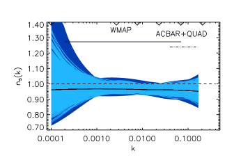
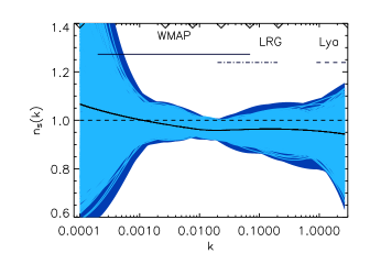
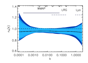
Our main results are presented in Fig. 3 for several data sets with increasing range in $k$: WMAP5 only, WMAP5 in combination with QUaD and ACBAR, and WMAP5 in combination with SDSS LRGs and Ly$\alpha$. We show the reconstructed $n_{s}(k)$ for ease of comparison with the standard power law results. However, the quantity that was actually reconstructed using cross-validation to find the optimal penalty is the power spectrum.

The optimal penalty for WMAP5 $\lambda_{\rm opt}^{\rm WMAP5}$ is higher than what was found for WMAP3 by a factor of $25$, and is consistent with the optimal penalty for WMAP3 in combination with CMB data at smaller scales Verde and Peiris (2008). The corresponding $n_{s}(k)$ is shown in the top left panel of Fig. 3. The same optimal penalty is found for WMAP5 and WMAP5$+$QUaD$+$ACBAR ($\lambda^{\rm WMAP5}_{\rm opt}=\lambda^{\rm CMB}_{\rm opt}$), and the latter reconstruction is shown in the top right panel of Fig. 3. For WMAP5$+$LRG$+$Ly$\alpha$, we find that CV becomes less sensitive to the value of the penalty, and the CV score dependence on the penalty flattens out at $\lambda_{\rm min}^{\rm WMAP5+LSS}=0.2\lambda^{\rm CMB}_{\rm opt}$. While this may indicate a preference for a less smooth $P(k)$, the data cannot distinguish between $\lambda_{\rm min}^{\rm WMAP5+LSS}$ and a penalty an order of magnitude higher. The reconstructed $n_{s}(k)$ are shown in the left and right bottom panels of Fig. 3 for penalties $\lambda_{\rm min}^{\rm WMAP5+LSS}$ and $10\lambda_{\rm min}^{\rm WMAP5+LSS}$, respectively. The dark and light blue regions enclose the best (ordered by likelihood) 95% and 68% reconstructions. The 95% constraints are not significantly broader than the 68% because the reconstructed spectra are simply more wiggly; they are not allowed by the data to deviate more from the best fit, consistently across scales.

Cross-validation is a useful tool to check for indications of unidentified systematic biases in the data. For example, in Ref. Verde and Peiris (2008) we found that the 3 year WMAP data (WMAP3) by itself favored a primordial power spectrum with a downward deviation from a power law at small scales (see Fig. 2 of Ref. Verde and Peiris (2008)). However, this feature disappeared when combining WMAP3 with other data sets (see Figs. 3 and 5 of Ref. Verde and Peiris (2008)) which overlapped WMAP3 on the scales corresponding to the feature – an inconsistency suggestive of a small residual systematic effect in the high $\ell$ WMAP3 data. Ref. Huffenberger et al. (2008) argued (based on considerations of frequency dependence) that the unresolved residual point source contribution to be subtracted from the raw $C_{\ell}$ should have been smaller by $28$% – and its uncertainty increased by 60% – compared to the WMAP3 official values. To judge if smoothing spline cross-validation could give some insights on possible residual systematic errors, we investigated how the point source subtraction level should have been changed for the aforementioned downturn at small scales to disappear from the reconstructed power spectrum. We obtained a point source amplitude $\sim 20$% lower than the WMAP estimated value, which is tantalizingly close to the estimate of Ref. Huffenberger et al. (2008).

In WMAP5, there is no longer any indication of deviations from a power-law primordial power spectrum, and the data require a smoother power spectrum (higher penalty) than WMAP3.

We find that WMAP5, CMB experiments at smaller scales, and the LRG power spectrum are all consistent with each other. With the addition of Ly$\alpha$ data, a lower penalty value is allowed. This could be a tentative indication of possible tension between Ly$\alpha$ and the other data sets, but not a very significant one: there is a cancellation between the effect of penalty and the effect of the likelihood over a wide range of penalty values as shown in the bottom panels of Fig. 3). In addition, as LRG and Ly$\alpha$ scales do not overlap, we cannot exclude the possibility of a low-significance local feature in the power spectrum.

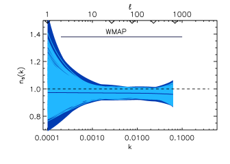
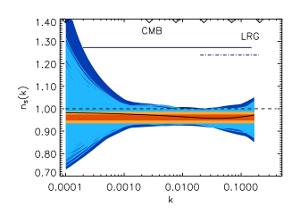
In Fig. 4 we show the reconstructed $n_{s}(k)$ for the CMB and LRG data, with optimal penalty $\lambda_{\rm opt}^{\rm WMAP5}$. The CV setup for WMAP5 is the same as before, LRGs are added in CV_A, and QUaD+ACBAR are included together in CV_B. We have excluded the Ly$\alpha$ data as it is the only non-overlapping data set. For comparison, we also show the 95% and 68% $n_{s}$ constraints Reid et al. (2009) for WMAP5$+$LRG data when a power-law spectral index is assumed to describe the shape of the primordial power spectrum. We see no evidence that any $k$-dependence of $n_{s}$ is necessary to describe the data in the CV reconstruction. While $n_{s}=1$ is disfavoured, the significance of the departure from scale invariance is weaker than when the “inflation-motivated” power law spectral index prior is adopted.

This minimally-parametric reconstruction highlights how constraints relax when generic forms of $P(k)$ are allowed. While this reconstruction is in agreement with the inflationary prior, it illustrates that better data are needed to justify its adoption observationally. Forthcoming data from Planck will significantly reduce the current reliance on priors in our understanding of the shape of the primordial power spectrum. Future large-scale structure data and Planck will overlap over a decade in scale, offering extra consistency checks. Lyman alpha data, on the other hand, offer the potential to extend the lever arm by at least another decade. We hope that the results presented here will form a basis to judge the robustness of our present knowledge when confronted with the precision measurements that are on the horizon.

Figure 4: Reconstructed spectral index $n_{s}(k)$ from WMAP5, ACBAR, QUaD and SDSS DR7 LRG data with optimal penalty determined from cross-validation excluding Ly$\alpha$. The orange-red band shows the 95% and 68% $n_{s}$ constraints Reid et al. (2009) for WMAP5$+$LRG data with a power-law prior.