Geometry-Temperature Interplay in the Casimir Effect

Abstract

We discuss Casimir phenomena which are dominated by long-range fluctuations. A prime example is given by “geothermal” Casimir phenomena where thermal fluctuations in open Casimir geometries can induce significantly enhanced thermal corrections. We illustrate the underlying mechanism with the aid of the inclined-plates configuration, giving rise to enhanced power-law temperature dependences compared to the parallel-plates case. In limiting cases, we find numerical evidence even for fractional power laws induced by long-range fluctuations. We demonstrate that thermal energy densities for open geometries are typically distributed over length scales of $1/T$. As an important consequence, approximation methods for thermal corrections based on local energy-density estimates such as the proximity-force approximation are expected to become unreliable even at small surface separations.

1 Introduction

Beyond its many attributes and genuine properties, the Casimir effect [1, 2, 3] is also a phenomenon that can be dominated by long-range fluctuations. At first sight, this statement may seem surprising as many standard Casimir examples do not show manifest signatures of a long-range fluctuation phenomenon (such as, e.g., critical phenomena). For instance, the length scale of fluctuations associated with the classic Casimir effect between parallel plates is certainly set by the plate separation $a$, serving effectively as a long-range cutoff.

Another seeming counter-example for the above-given statement is the sphere-plate configuration at small separation distances $a$, which is experimentally highly relevant [4]. Here, the Casimir interaction energy behaves as $E\sim R/a^{2}$ for $a/R\to 0$, where $R$ is the sphere radius. It thus exhibits a simple power law with integer coefficients that follow from a geometric scaling analysis known as the proximity force approximation (PFA) [5]. (The validity of this approximation in the asymptotic regime has been confirmed by analytical as well as numerical methods of quantum field theory [6, 7, 8, 9, 10], see also Ref. Bulgac:2005ku for a solution at larger distances.) Similar geometric analyses work equally well for, say, electrostatic forces in the same configuration which are not related to any long-range fluctuation phenomenon.

In the present work, we argue that these examples do not reveal the long-range nature of the Casimir effect, as the corresponding interaction energies are dominated by rather localized energy densities. E.g., for the sphere-plate case, the dominant contribution to the Casimir force arises from the region between the surfaces at closest separation. By contrast, we present Casimir phenomena in the following where the energy density is distributed over a wide range of scales, such that the potential long-range nature of the Casimir effect becomes most prominent.

An example of this class of phenomena is the nontrivial interplay of finite-temperature and geometry dependences of the Casimir effect. As first conjectured in Ref. Scardicchio:2005di, the thermal modifications of the Casimir effect can differ qualitatively for different geometries. This is because the thermal corrections arise from thermal excitations of the fluctuation spectrum, which in turn depends strongly on the geometry. First analytical as well as numerical evidence of this “geothermal” interplay has been provided in Ref. Gies:2008zz by applying the worldline formalism to a perpendicular-plates configuration. A detailed study of this phenomenon for the more general inclined-plates case has been performed in Ref. Weber:2009dp, the results of which will be used as a quantitative example for our arguments in the following.

The purpose of the present contribution is to develop the general physics picture underlying the geothermal Casimir phenomena. In Sect. 2, we discuss the origin and various general perspectives on the interplay between geometry and finite temperature. Section 3 briefly summarizes the worldline method which is a powerful tool to analyze this interplay quantitatively. Several examples will be discussed in Sect. 4, where we also present new results for the thermal force density of specific open geometries. Conclusions are given in Sect. 5.

2 Origin of geothermal Casimir phenomena

The origin of a nontrivial interplay between geometry and temperature in the Casimir effect can be understood in simple terms. Consider the classical parallel-plate case: as the wavelengths of the fluctuations orthogonal to the plates have to be commensurate with the distance $a$ between the plates, this corresponding relevant part of the spectrum $\omega_{n}^{2}(a)=p_{\|}^{2}+(\pi n/a)^{2}$ has a gap of wave number $k_{\text{gap}}=\pi/a$. As is obvious, e.g., from the partition function $Z=\sum_{n}\exp(-\omega_{n}(a)/T)$, the gapped modes are exponentially suppressed at small temperatures $T\ll k_{\text{gap}}$. In $D=4$ spacetime dimensions, the integration over the parallel modes $p_{\|}$ converts this exponential dependence into the low-temperature power law $T^{4}$ for the parallel-plate Casimir force. The corresponding thermal contribution to the interaction energy (apart from a distance-independent term) is

$$\Delta E_{\|}(T)=\frac{\pi^{2}}{90}\,A\,a\,T^{4},\quad aT\ll 1,$$ (1)

where $A$ denotes the plate’s area. The above-given argument for a suppression of thermal contributions applies to all geometries with a gap in the relevant part of the spectrum (e.g. concentric cylinders or spheres, Casimir pistons, etc.). These geometries are called closed.

By contrast, open geometries with a gapless relevant part of the spectrum have no such suppression of thermal contributions. Any small value of the temperature can always excite the low-lying modes in the spectrum. Therefore, we expect a generically stronger thermal contribution $\sim(aT)^{\alpha}$ with $0<\alpha<4$.

Another argument for the fundamental difference between open and closed geometries and thermal corrections is the following: Eq. (1) can also be written as $\Delta E_{\|}(T)=V\,\epsilon_{\text{SB}}$, where $V=aA$ is the volume between the parallel plates, and $\epsilon_{\text{SB}}$ is the Stefan-Boltzmann free energy density of the radiation field. Hence, we can understand the low-temperature correction in the parallel-plate case as an excluded volume effect: the thermal modes of the radiation field at low temperatures do not fit in between the plates, and therefore the corresponding volume does not contribute to the total thermal free energy. By contrast, open geometries by construction cannot be associated with any (unambiguously defined) excluded volume, such that significant deviations from a $T^{4}$ behavior can be expected.

These considerations immediately point to the possibility that the thermal part of the low-temperature Casimir effect can be dominated by long-range fluctuations. This is because a temperature much lower than the inverse distance, $aT\ll 1$, sets a new length scale which can be much larger as the plate distance as well as any other length scale of the geometry (such as a sphere radius). In closed geometries, this length scale is effectively cut off by the gap in the spectrum, implying the parametric suppression of thermal effects. In open geometries, this length scale sets a relevant scale that can, for instance, reflect the spatial extent of the distribution of the thermal energy density. The total thermal energy thus can receive dominant contributions from long-range modes corresponding to significantly extended thermal energy distributions.

An important consequence can already be anticipated at this point: approximation methods that are based on local considerations will generically fail to predict the correct low-temperature correction in open geometries. An example is given by the PFA which is based on the assumption that the Casimir energy can be estimated by integrating over local parallel-plates energy densities. Whereas this approximation may or may not work at zero temperature depending on the geometric details of the configuration, it is even conceptually questionable at finite temperature, as open geometries should not be approximated by closed-geometry building blocks. Quantitatively, such a procedure is expected to fail, as local energy-density approximations will not be able to capture the contributions from larger length scales induced by long-range modes.

The temperature-geometry interplay is not an academic problem: experimentally important configurations such as the sphere-plate or the cylinder-plate geometry belong to this class of open geometries, but thermal corrections have so far been approximated by the PFA. Whether or not a potentially significant geothermal interplay may exist in the relevant parameter range $aT\sim 0.01\dots 0.1$ is a technically challenging quantitative problem.

The considerations so far have concentrated on the low-temperature limit. In fact, the high-temperature limit exhibits a universal linear dependence on the temperature for a simple reason. At high temperature in the imaginary-time formalism, only the zeroth Matsubara mode can contribute as all higher modes acquire thermal masses $\sim\pi T$ and hence are largely suppressed. The zeroth Matsubara mode has no temperature dependence at all, such that the only temperature dependence arises from the measure of the fluctuation trace which is linear in $T$. A less technical argument with the same result can be based on the underlying Bose-Einstein distribution governing the bosonic thermal fluctuations of the radiation field. This distribution increases as $\sim{T}$ in the high-temperature limit, inducing this linear temperature dependence directly in the thermal energy. The properties of the geometry only enter the prefactor in the high-temperature limit. Universal features of thermal Casimir energies with an emphasis on the high-temperature limit have been systematically studied in Refs. Balian:1977qr,Klich:2000qm,Nesterenko:2000cf,Bordag:2001jc.

3 Worldline method for the Casimir effect

Let us briefly review the worldline approach[20] to the Casimir effect as it is needed for the present line of argument. For the remainder of the paper, we consider a fluctuating massless scalar field satisfying Dirichlet boundary conditions on the Casimir surfaces. For details of the formalism, see Refs. Gies:2003cv,Gies:2006cq,Weber:2009dp. Consider a configuration $\Sigma$ consisting of two static surfaces $\Sigma_{1}$ and $\Sigma_{2}$. The worldline representation of the Casimir interaction energy reads

$$E_{\mathrm{c}}=-\frac{1}{2(4\pi)^{D/2}}\!\int_{0}^{\infty}\!\!\!\frac{\mathrm{d}\mathcal{T}}{\mathcal{T}^{1+D/2}}\!\int\!\mathrm{d}^{d}x_{\mathrm{CM}}\left\langle\Theta_{\Sigma}[\mathbf{x}(\tau)]\right\rangle,$$ (2)

where $D=d+1$ denotes the spacetime dimensions. The worldline functional obeys $\Theta_{\Sigma}[\mathbf{x}]=1$ if a worldline $\mathbf{x}(\tau)$ intersects both surfaces $\Sigma=\Sigma_{1}\cup\Sigma_{2}$, and is zero otherwise.

The expectation value in Eq. (2) is taken with respect to an ensemble of $d$-dimensional closed Gaußian worldlines with center of mass $\mathbf{x}_{\mathrm{CM}}$,

$$\langle\dots\rangle=\frac{\int_{\mathbf{x}_{\text{CM}}}\mathcal{D}\mathbf{x}\,\dots\,e^{-\frac{1}{4}\int_{0}^{\mathcal{T}}\mathrm{d}\tau\,\dot{\mathbf{x}}^{2}(\tau)}}{\int_{\mathbf{x}_{\text{CM}}}\mathcal{D}\mathbf{x}\,e^{-\frac{1}{4}\int_{0}^{\mathcal{T}}\mathrm{d}\tau\,\dot{\mathbf{x}}^{2}(\tau)}}.$$ (3)

Equation (2) expresses the fact that all worldlines intersecting both surfaces do not satisfy Dirichlet boundary conditions on both surfaces. They are removed from the ensemble of allowed fluctuations by the $\Theta$ functional and thus contribute to the negative Casimir interaction energy. The auxiliary propertime parameter $\mathcal{T}$ scales the extent of a worldline by a factor of $\sqrt{\mathcal{T}}$. Large $\mathcal{T}$ correspond to long-range, small $\mathcal{T}$ to short-range fluctuations.

Finite temperature $T=1/\beta$ in the Matsubara formalism is equivalent to a compactified Euclidean time on the interval $[0,\beta]$. The worldlines now live on $S^{1}\times\mathbbm{R}^{d}$ and can carry a winding number. Summing over all winding numbers, the Casimir energy (2) becomes

$$E_{\mathrm{c}}=-\frac{1}{2(4\pi)^{D/2}}\int_{0}^{\infty}\!\!\!\frac{\mathrm{d}\mathcal{T}}{\mathcal{T}^{1+D/2}}\!\!\left(1+2\sum_{n=1}^{\infty}\!e^{-\frac{n^{2}\beta^{2}}{4\mathcal{T}}}\right)\!\!\int\!\mathrm{d}^{d}x_{\mathrm{CM}}\left\langle\Theta_{\Sigma}[\mathbf{x}(\tau)]\right\rangle.$$ (4)

The finite-temperature worldline formalism for static configurations thus boils down to an additional winding-number prefactor in front of the worldline expectation value. Notice that the winding-number sum is directly related to the standard Matsubara sum by a Poisson resummation.

Finally, it is advantageous to rescale the worldlines such that the velocity distribution becomes independent of $\mathcal{T}$,

$$\boldsymbol{\gamma}(t):=\frac{1}{\sqrt{\mathcal{T}}}\mathbf{x}(\mathcal{T}t)\quad\!\!\!\to\!\!\!\quad e^{-\frac{1}{4}\int_{0}^{\mathcal{T}}\dot{\mathbf{x}}^{2}\mathrm{d}\tau}=e^{-\frac{1}{4}\int_{0}^{1}\dot{\boldsymbol{\gamma}}^{2}\mathrm{d}t},$$ (5)

where $\dot{\boldsymbol{\gamma}}=\mathrm{d}\boldsymbol{\gamma}(t)/\mathrm{d}t$. The worldline integrals can be evaluated also numerically by Monte Carlo methods in a straightforward manner. Various efficient ab initio algorithms for generating discretized worldlines with Gaußian velocity distribution have been developed, see, e.g., Refs. Gies:2003cv,Gies:2005sb.

4 Geothermal phenomena for inclined Casimir plates

4.1 Inclined plates at zero temperature $T=0$

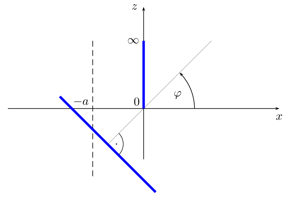
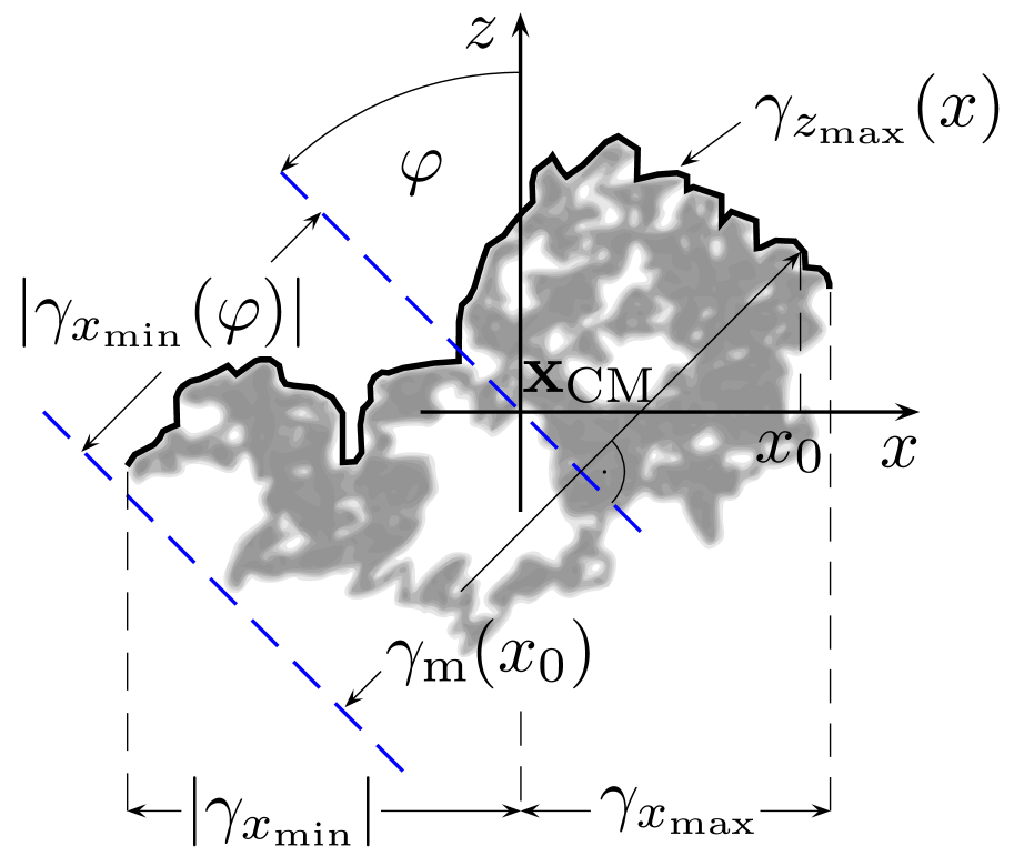
Figure 1: Left panel: sketch of the inclined-plates configuration. The infinite plate (dashed line) is rotated in the $x,z$ plane by an angle $\varphi$. As special cases, $\varphi=0$ corresponds to the configuration of one semi-infinite plate parallel to an infinite plate (1si configuration), whereas $\varphi=\pi/2$ yields the perpendicular-plates configuration. Right panel: all relevant information for the evaluation of the Casimir energy (6) of inclined plates is encoded in the function $\gamma_{\mathrm{m}}(x)$, which has to be integrated from $\gamma_{x_{\mathrm{min}}}$ to $\gamma_{x_{\mathrm{max}}}$.

The inclined-plates (i.p.) configuration turns out to be an ideal work horse to study geothermal phenomena, in particular, the transition from open to closed geometries and the role of long-range fluctuations. It was studied in detail in Ref. Weber:2009dp for general $D$. Very recently, results for inclined plates have been obtained for the electromagnetic case at zero temperature using scattering theory[15]. Here, we summarize our results for $D=4$ and provide more details on the geometry-temperature interplay.

The inclined-plates configuration consists of a perfectly thin semi-infinite plate above an infinite plate at an angle $\varphi$, see Fig. 1. The semi-infinite plate has an edge of length $L_{y}$. The area of the infinite plate is $A$. The limit $L_{y},\,A\to\infty$ is implicitly understood. Let $a$ be the minimal distance between the plates. Evaluating the $\Theta$ functional for this configuration [14] in (2), the Casimir energy can be written as

$$\frac{E_{\mathrm{c}}^{\mathrm{i.p.,\varphi}}}{L_{y}}= -\frac{\csc(\varphi)}{96\,\pi^{2}\,a^{2}}\left\langle\int_{\gamma_{x_{\mathrm{min}}}}^{\gamma_{x_{\mathrm{max}}}}\mathrm{d}x\ \gamma_{\mathrm{m}}^{3}(x)\right\rangle,$$ (6)

where

$$\gamma_{\mathrm{m}}(x) \equiv x\cos(\varphi)+\sin(\varphi)\gamma_{z_{\mathrm{max}}}(x)-\gamma_{x_{\mathrm{min}}}(\varphi),$$ (7)

$$\gamma_{{x_{\mathrm{min}}}}(\varphi) \equiv\min_{t}\left(\gamma_{{x}}(t)\cos(\varphi)+\gamma_{z}(t)\sin(\varphi)\right).$$ (8)

Here, the Casimir energy has been related to simple geometrical properties of the worldlines: $\gamma_{{x_{\mathrm{min}}}}(\varphi)$ measures the extent of the worldline in the negative $x$ direction of a coordinate system rotated by the angle $\varphi$, and $\gamma_{z_{\text{max}}}(x)$ denotes the $x$-dependent envelope of the worldline in positive $z$ direction, see Fig. 1. Equation (6) is shown as a function of $\varphi$ in Fig. 2.

For $\varphi=\pi/2$ we rediscover the perpendicular plates result [23, 24] as a special case. For $\varphi=0$, the integral in Eq. (6) can be done analytically resulting in $\langle\lambda^{4}/4\rangle=\pi^{4}/30$. Together with the $\varphi$-dependent prefactor, Eq. (6) diverges as $\varphi\rightarrow 0$ as it should. This is because Eq. (6) corresponds to the energy per unit edge length, whereas for $\varphi\to 0$ the Casimir energy becomes proportional to the area of the semi-infinite plate.

The result for the parallel limit $\varphi\rightarrow 0$ has to arise from the general inclined-plates formula Eq. (6), but involves a subtle limiting process which was performed in Ref. Weber:2009dp. For this 1si case, the total Casimir interaction energy decomposes into [23, 24],

$$E_{\mathrm{c}}^{\mathrm{1si}}=E_{\mathrm{c}}^{\mathrm{1si,\parallel}}+E_{\mathrm{c}}^{\mathrm{1si,edge}},$$ (9)

where $E_{\mathrm{c}}^{\mathrm{1si,\parallel}}/A$ is the usual Casimir energy per unit area of two parallel plates, with $A$ now being the area of the semi-infinite plate. The subleading edge energy $E_{\mathrm{c}}^{\mathrm{1si,edge}}$ arises solely due to the presence of the edge and is proportional to the length of the latter. For finite plates, the edge effect contributes to the Casimir force, effectively increasing the plates’ area [23, 14].

The Casimir torque ${D_{\mathrm{c}}^{\mathrm{i.p.,\varphi}}}$ can easily be obtained from

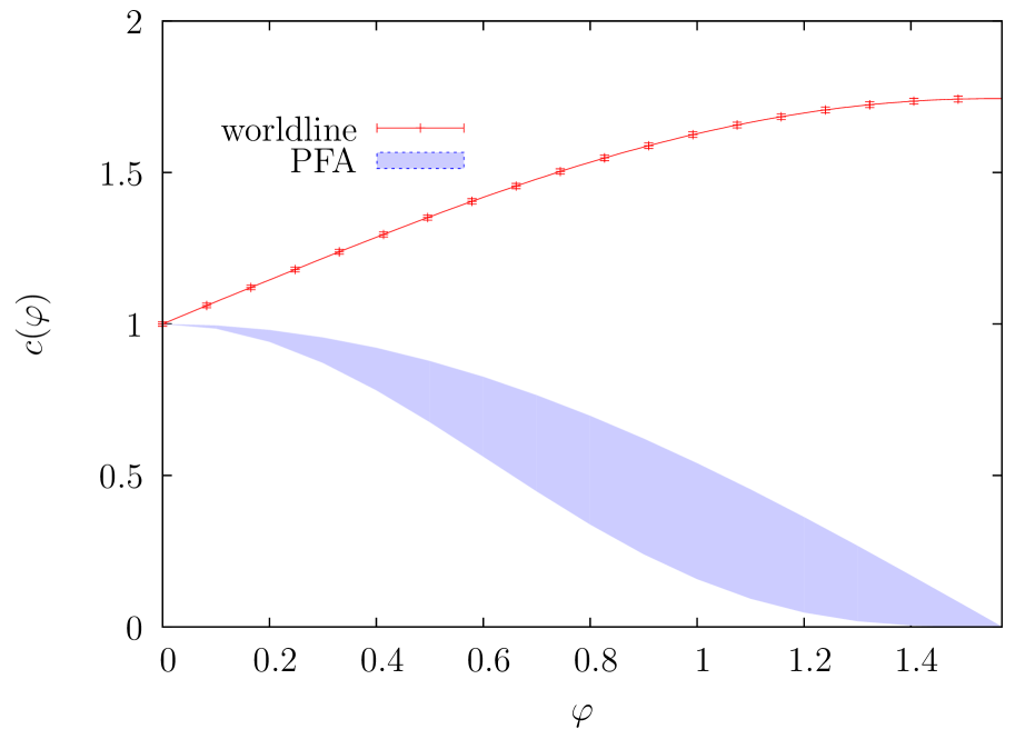
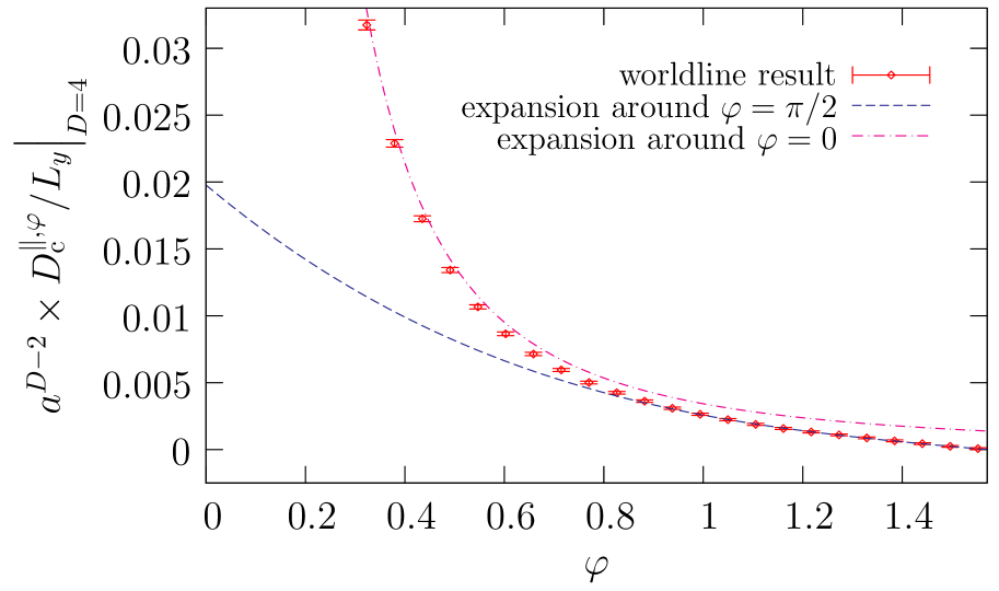
Figure 2: Left panel: normalized Casimir energy per edge length of the inclined-plates configuration, $c(\varphi)=-2880E_{\mathrm{c}}^{\mathrm{i.p.,\varphi}}a^{2}\sin(\varphi)/\pi^{2}L_{y}$. The blue area corresponds to the PFA prediction: for the upper bound, we have used the infinite plate as a basis, for the lower bound the semi infinite plate, yielding $\cos(\varphi)$ and $\cos^{3}(\varphi)$ as bounding curves, respectively. Right panel: normalized Casimir torque per edge length (Eq. 10) and its expansion around $\varphi=\pi/2$ (Eq. (11)) and $\varphi=0$ (Eq. (12)), respectively.

$${D_{\mathrm{c}}^{\mathrm{i.p.,\varphi}}}=\frac{\mathrm{d}E_{\mathrm{c}}^{\mathrm{i.p.,\varphi}}}{\mathrm{d}\varphi}.$$ (10)

Fitting the numerical data for the torque to an odd polynomial in the vicinity of $\varphi\to\pi/2$, we obtain (see Fig. 2)

$$\frac{{D_{\mathrm{c}}^{\mathrm{i.p.,\varphi\rightarrow\pi/2}}}a^{2}}{L_{y}}\approx 0.00329\left(\frac{\pi}{2}-\varphi\right)+0.0038\left(\frac{\pi}{2}-\varphi\right)^{3}.$$ (11)

For the other limit $\varphi\!\rightarrow\!0$, the Casimir torque diverges. The leading order[14],

$${D_{\mathrm{c}}^{\mathrm{i.p.,\varphi\rightarrow 0}}}\cong\frac{L_{y}\pi^{2}}{2880a^{2}\varphi^{2}}\approx 0.00343\frac{L_{y}}{a^{2}\varphi^{2}},$$ (12)

is an excellent approximation to Eq. (10) for $\varphi$ not too close to $\pi/2$. The divergent Casimir torque per length can be converted into a finite torque per unit area which leads to the classical result for the torque,

$$D_{\mathrm{c}}^{\mathrm{\parallel,\varphi\rightarrow 0}}=\frac{AL_{z}\pi^{2}}{960a^{4}}\approx 0.0103\frac{AL_{z}}{a^{4}}.$$ (13)

Here, $A$ and $L_{z}$ denote the semi-infinite plate’s area and the extent in $z$ direction, respectively.

A new characteristic contribution emerges from the edge effect Eq. (9) which effectively changes the shape of the upper plate seen by worldlines, as the upper plate appears to be higher near and at the edge itself. This leads to a contribution which works against the standard torque (13). The correction to Eq. (13) emerging from the edge effect then is[14] $\approx-(0.003660\pm 0.000038)L_{y}/a^{2}$.

4.2 Inclined plates at finite temperature

Decomposing the Casimir free energy at finite temperature $T=1/\beta$ into its zero-temperature part $E_{\mathrm{c}}(0)$ and finite-temperature correction $\Delta E_{\mathrm{c}}(T)$,

$$E_{\mathrm{c}}(T)=E_{\mathrm{c}}(0)+\Delta E_{\mathrm{c}}(T),$$ (14)

is straightforward in the worldline picture by using the relation (4). The finite-temperature correction is purely driven by the worldlines with nonzero winding number, whereas the complicated geometry-dependent part of the calculation remains the same for zero or finite temperature. The same statement holds for the Casimir force $F_{\mathrm{c}}(T)=F_{\mathrm{c}}(0)+\Delta F_{\mathrm{c}}(T)$.

In the following, we concentrate on the low-temperature limit, $aT\ll 1$. Full expressions for arbitrary temperature can be found in Ref. Weber:2009dp. From dimensional analysis of Eq. (14), we would naively expect the Casimir energy to be of the form

$$E_{\mathrm{c}}(T)=E_{\mathrm{c}}(0)(1+c_{1}aT+c_{2}(aT)^{2}+c_{3}(aT)^{3}+\dots).$$ (15)

No negative exponents should appear in (15) since the thermal part of the energy has to disappear as $T\rightarrow 0$. Generically, the $T=0$ Casimir energy $E_{\mathrm{c}}(0)$ diverges for surfaces approaching contact $a\to 0$. From Eq. (15), we would naively expect the same for the thermal correction. If, however, sufficiently many of the first $c_{i}$’s in Eq. (15) vanish, then the thermal part of the Casimir energy will be well behaved in $a$ without a divergence for $a\rightarrow 0$.

This is indeed the case for parallel plates ($c_{1}=c_{2}=0$, and $E_{\mathrm{c}}(0)\sim 1/a^{3}$) and for inclined plates ($c_{1}=0$, and $E_{\mathrm{c}}(0)\sim 1/a^{2}$). As a consequence, an extreme simplification arises: the thermal contribution in the low-temperature limit can be obtained by first taking the formal limit $a=0$ (only in the thermal contribution, of course).

In the following, we argue that there is no divergence in the thermal contribution in the limit $a\to 0$ for general geometries: Imagine a fancy geometry. The $a$-divergent part arises from the regions near the points (or lines or surfaces) of contact as $a\rightarrow 0$. The surfaces in these regions by construction bend away from each other. The thermal contribution can now be made larger by flattening the surfaces in the contact region. Let us now substitute these regions by broader parallel plates. Then, the local thermal contribution to the Casimir energy of the original configuration will be clearly smaller than the finite thermal contribution of parallel plates. As the latter does not lead to divergences for $a\to 0$, there can also be no divergence for the general curved case arising from the contact regions. Of course, infinite geometries may still experience an infinite thermal force, as it is the case for two infinitely extended parallel plates, but the local thermal contribution to the force density will be finite.

Another distinct feature of low-temperature effects is the spread of the thermal force density over regions of size $\sim 1/T$ even for very small separations $a$. These effects are, of course, relevant for open geometries such as a sphere and cylinder above a plate[25]. But it can also be demonstrated by calculating the thermal force density $\Delta f_{\mathrm{c}}(r,T)=f_{\mathrm{c}}(r,T)-f_{\mathrm{c}}(r,0)$ for two perpendicular plates at a distance $a=0$ as a function of the coordinate $r$ on the infinite surface measuring the distance from the edge (i.e., the contact point). The result can easily be obtained fully analytically on the worldline[25], yielding

$$\Delta f_{\mathrm{c}}(r,T)=-\frac{T^{4}L_{y}}{2\pi^{2}}\!\left[\frac{\pi^{4}}{45}-\!\sum_{n=1}^{\infty}\!\left\langle\frac{2e^{-(n\lambda_{1}/2rT)^{2}}}{n^{4}}-\frac{\lambda_{1}^{2}e^{-(n\lambda_{1}/2rT)^{2}}}{2T^{2}n^{2}r^{2}}\right\rangle\right],$$ (16)

where $\lambda_{1}$ measures the extent of half a unit worldline, i.e., the distance measured in $x$ direction from the left end to the center of mass. Rescaling the radial coordinate $r\rightarrow\lambda_{1}r$ per worldline, the following rescaled force density leads to the same force upon integration over $r$,

$$\Delta\tilde{f}_{\mathrm{c}}(r,T)=-\frac{T^{4}L_{y}\sqrt{\pi}}{4\pi^{2}}\left[\frac{\pi^{4}}{45}-\sum_{n=1}^{\infty}\left(\frac{2e^{-(n/2rT)^{2}}}{n^{4}}-\frac{e^{-(n/2rT)^{2}}}{2T^{2}n^{2}r^{2}}\right)\right],$$ (17)

where we have used $\langle\lambda_{1}\rangle=\sqrt{\pi}/2$. (Equations (16) and (17) possibly differ by a total derivative, but both provide for a reasonable thermal force density.) Upon integration, we obtain the thermal force of the perpendicular plates at $a=0$, $\Delta F_{\mathrm{c}}(T)=-\zeta(3)\,L_{y}T^{3}/4\pi$ in agreement with Ref. Gies:2008zz. In the limit $a\to 0$, the configuration has a scale invariance, which is reflected in the fact that Eqs. (16, 17) remain unchanged under $T\rightarrow T\alpha,\ r\rightarrow r/\alpha$ and $\Delta\tilde{f}_{\mathrm{c}}\rightarrow\Delta\tilde{f}_{\mathrm{c}}/\alpha^{4}$ for arbitrary $\alpha$. That means that evaluating (16, 17) for say $T=1$ is sufficient to infer its form at all other $T$. Equation (17) is shown for $T=1$ in Fig. 3. The inflection point of each term in the $n$ sum is at $r_{0}=n/T\sqrt{10}$. For $r<1/T\sqrt{10}$ the force density stays nearly constant (and is equal to the first term in (16)) and rapidly goes to zero for $r>1/T\sqrt{10}$. From this, we draw the important conclusion, that the region of constant force density can be made arbitrarily large in $r$ direction by choosing sufficiently low $T$.

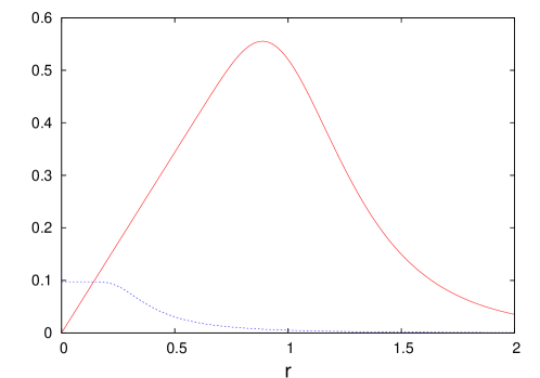
Figure 3: The negative rescaled thermal force density Eq. (17) for perpendicular plates (dashed blue line) and the negative radial thermal force density for a sphere of radius $R=1$ above an infinite plate (solid red line) for $T=1$. The thermal force density in the sphere-plate case has a maximum of $\approx 2\pi\times\pi^{2}/90$, where the factor $2\pi$ arises from the cylindrical measure. Note that a considerable fraction of the force density lies outside the sphere which only extends to $r=1$. As temperature drops, the maximum moves monotonously to the right.

Similar important consequences arise for temperature effects in other geometries. For example, the radial force density of a sphere above a plate exhibits a maximum due to the cylindric measure factor $r$, see Fig. 3. Although this force density is not scale invariant due to the additional dimensionful scale $R$ (sphere radius), its maximum will nevertheless move away from the sphere as the temperature drops. No local approximate tools such as the PFA will be able to predict the correct thermal force. The fact that the force density is not scale invariant leads to different temperature behaviors for $T<1/R$ and $T>1/R$ even in the limit $a\rightarrow 0$. [25]

Let us now compare the low-temperature limit of the Casimir energy of two inclined plates with that of two parallel plates. For $(aT)\rightarrow 0$, the correction $\Delta E^{\parallel}_{\mathrm{c}}$ to the well-known parallel-plates energy reads

$$\frac{\Delta E^{\parallel}_{\mathrm{c}}(aT\rightarrow 0)}{A}=-\frac{\zeta(3)T^{3}}{4\pi}+\frac{\pi^{2}aT^{4}}{90}\approx-0.0957T^{3}+0.110aT^{4}.$$ (18)

Note that only the $T^{4}$ term contributes to the force. The thermal correction to the inclined-plates energy is much more sensitive to temperature,

$$\frac{\Delta E_{\mathrm{c}}^{\mathrm{i.p.},\varphi}(aT\rightarrow 0)}{L_{y}}=-\frac{c_{\varphi,T_{0}}T^{2}}{24\sin(\varphi)}+\frac{\zeta(3)aT^{3}}{4\pi\sin(\varphi)},$$ (19)

where $c_{\varphi,T_{0}}$ was calculated numerically in Ref. Weber:2009dp as a function of $\varphi$. Only the second term, which is a purely analytical result, contributes to the force. Equation (19) is the generalization of a result for perpendicular plates, $\varphi=\pi/2$, see Ref. Gies:2008zz.

Equation (19), being an energy per edge length, diverges as $\varphi\rightarrow 0$. As in Eq. (9), it has to be replaced by the energy of a semi-infinite plate above a parallel one, $E_{\mathrm{c}}^{\mathrm{1si}}(T)=E_{\mathrm{c}}^{\mathrm{1si,edge}}(T)+E_{\mathrm{c}}^{\mathrm{1si,\parallel}}(T)$. The thermal part of $E_{\mathrm{c}}^{\mathrm{1si,\parallel}}(T)$ is as in Eq. (18), where $A$ is the area of the semi-infinite plate. The leading thermal correction to the edge effect $\Delta E_{\mathrm{c}}^{\mathrm{1si,edge}}(T)$ reads

$$\frac{\Delta E_{\mathrm{c}}^{\mathrm{1si,edge}}(T)}{L_{y}}=-\frac{c_{\varphi,T_{0}}T^{2}}{24}+0.063a^{1.74}T^{3.74}.$$ (20)

We find that the low-temperature regime of the 1si edge effect is well described by a non-integer power law, $\Delta F_{\text{c}}^{\text{1si,edge}}\sim T^{3.74}$, where the fractional exponent arises from the geometry-temperature interplay in this open geometry. Of course, our numerical analysis cannot guarantee to determine the true asymptotic behavior in the limit $aT\to 0$, but our data in the low-temperature domain $0.01\lesssim aT\lesssim 0.4$ are well fitted by the non-integer scaling also at higher fit orders[14]. This result is very reminiscent to non-integer exponents known from critical phenomena. In both cases, this result arises from fluctuation contributions on all length scales, clearly revealing the long-range nature of both phenomena. Note that the leading temperature exponent of the 1si geometry is between the parallel-plates exponent $4$ and the inclined-plates exponent $3$, reflecting the fact that thermal properties of the 1si geometry lie between those of the parallel and inclined plates.

The long-range nature of Casimir phenomena becomes also visible at the thermal correction to the torque. This is immediately transparent from Eq. (19). Whereas the $a$-independent first term of Eq. (19) does not contribute to the force, both terms in Eq. (19) contribute to the low-temperature limit of the Casimir torque, the thermal contribution being $\mathrm{d}\Delta E_{\mathrm{c}}^{\mathrm{i.p.,\varphi}}(T)/\mathrm{d}\varphi$. Concentrating on the limit $aT\rightarrow 0$ for small deviations from the perpendicular-plates case, $\varphi=\pi/2{-}\delta\varphi$, an expansion to first order in $\delta\varphi$ yields:

$$\Delta D_{\mathrm{c}}^{\mathrm{i.p.},\varphi=\pi/2-\delta\varphi}(aT\rightarrow 0)/L_{y}=\left(0.0716-0.0957aT\right)T^{2}\delta\varphi.$$ (21)

In the validity regime of the low-temperature expansion, $aT\ll 1$, the positive first term is always dominant, hence the perpendicular-plates case remains a repulsive fixed point. Most importantly, we would like to stress that the quadratic dependence of the torque on the temperature $\sim T^{2}$ ($\sim T^{D-2}$ in the general case) for the inclined-plates configuration represents the strongest temperature dependence of all observables discussed here.

5 Conclusions

A nontrivial interplay between finite temperature fluctuations and the geometry of a configuration can give rise to a variety of qualitatively different thermal corrections to Casimir phenomena. This effect becomes most pronounced in geometries where the relevant part of the spectrum is gapless. In these so-called open geometries, any small value of the temperature can excite low-lying thermal modes, giving rise to thermal corrections. By contrast, a gap in the relevant part of the spectrum of closed geometries suppresses thermal excitations at low temperature.

In the present work, we have developed the general picture underlying these geothermal Casimir phenomena. Open geometries, for instance, support a stronger influence of long-range fluctuations on thermal Casimir phenomena. We have illustrated the underlying mechanisms with the aid of the inclined-plates configuration and also presented first results for the experimentally important sphere-plate configuration.

Furthermore, we have presented a general argument that low-temperature corrections to Casimir forces become much more easily accessible by taking the (formal) contact limit $a\to 0$ (only for the thermal contributions), as thermal corrections remain well behaved in this limit. Whereas the existence of this limit is well known for parallel plates, we have argued that the same result holds for general geometries. The existence of this limit is also a reason why thermal corrections, for instance, in the perpendicular-plate case can be determined analytically. We expect that this observation will be useful for many other geometries as well. This should lead to practical simplifications also in other field theory approaches such as functional-integral approaches[26, 27], scattering theory[28, 29, 30, 31, 32], and mode summation[33].

This particular geothermal interplay which we have observed in the context of the Casimir effect is certainly not restricted to Casimir physics. The crucial ingredients are a gapless fluctuation spectrum (though small gaps may not necessarily exert a strong quantitative influence) in a spatially inhomogeneous background. We expect that similar phenomena can occur for the thermal response of a system with an inhomogeneous condensate and an (almost) gapless fluctuation spectrum.

We conclude with the remark the geothermal interplay is only one out of several highly nontrivial interferences between deviations from the ideal Casimir limit. For instance, the interplay between dielectric material properties and finite temperature [34] is still a subject of intense theoretical investigations and has created a long-standing controversy [35, 36, 37, 38, 39]. Also the interplay between dielectric properties and geometry has been shown to lead to significant deviations from ideal curvature effects as well [40]. All this exemplifies that a profound understanding of the Casimir effect requires a thorough quantum field theoretic basis.

Acknowledgments: We would like to thank Kim Milton and all organizers of QFEXT09 for creating such a stimulating and productive conference atmosphere. This work was supported by the National Science. We have benefited from activities within the ESF Research Network CASIMIR and acknowledge support from the Landesgraduiertenförderung Baden-Württemberg, the Heidelberg Graduate School of Fundamental Physics (AW), and from the DFG grant Gi328/5-1 and SFB-TR18 (HG).

References

- [1] H.B.G. Casimir, Kon. Ned. Akad. Wetensch. Proc. 51, 793 (1948).
- [2] M. Bordag, U. Mohideen and V. M. Mostepanenko, Phys. Rept. 353, 1 (2001); R. Onofrio, New J. Phys. 8, 237 (2006) [arXiv:hep-ph/0612234]; S. Y. Buhmann and D. G. Welsch, Prog. Quant. Electron. 31, 51 (2007) [arXiv:quant-ph/0608118].
- [3] K. A. Milton, “The Casimir effect: Physical manifestations of zero-point energy,” River Edge, USA: World Scientific (2001).
- [4] S. K. Lamoreaux, Phys. Rev. Lett. 78, 5 (1997); U. Mohideen and A. Roy, Phys. Rev. Lett. 81, 4549 (1998); H.B. Chan et al., Science 291, 1941 (2001); R.S. Decca et al., Phys. Rev. D 68, 116003 (2003); Phys. Rev. Lett. 94, 240401 (2005).
- [5] B.V. Derjaguin, I.I. Abrikosova, E.M. Lifshitz, Q.Rev. 10, 295 (1956); J. Blocki, J. Randrup, W.J. Swiatecki, C.F. Tsang, Ann. Phys. (N.Y.) 105, 427 (1977).
- [6] M. Schaden and L. Spruch, Phys. Rev. A 58, 935 (1998); Phys. Rev. Lett. 84 459 (2000)
- [7] H. Gies, K. Langfeld and L. Moyaerts, JHEP 0306, 018 (2003); arXiv:hep-th/0311168.
- [8] A. Scardicchio and R. L. Jaffe, Nucl. Phys. B 704, 552 (2005); Phys. Rev. Lett. 92, 070402 (2004).
- [9] H. Gies and K. Klingmuller, Phys. Rev. Lett. 96, 220401 (2006) [arXiv:quant-ph/0601094].
- [10] M. Bordag, Phys. Rev. D 73, 125018 (2006); Phys. Rev. D 75, 065003 (2007).
- [11] A. Bulgac, P. Magierski and A. Wirzba, Phys. Rev. D 73, 025007 (2006) [arXiv:hep-th/0511056]; A. Wirzba, A. Bulgac and P. Magierski, J. Phys. A 39 (2006) 6815 [arXiv:quant-ph/0511057].
- [12] A. Scardicchio and R. L. Jaffe, Nucl. Phys. B 743 (2006) 249 [arXiv:quant-ph/0507042].
- [13] H. Gies and K. Klingmuller, J. Phys. A 41, 164042 (2008).
- [14] A. Weber and H. Gies, Phys. Rev. D 80, 065033 (2009) [arXiv:0906.2313 [hep-th]].
- [15] N. Graham, A. Shpunt, T. Emig, S. J. Rahi, R. L. Jaffe and M. Kardar, arXiv:0910.4649 [quant-ph].
- [16] R. Balian and B. Duplantier, Annals Phys. 112, 165 (1978).
- [17] I. Klich, J. Feinberg, A. Mann and M. Revzen, Phys. Rev. D 62, 045017 (2000) [arXiv:hep-th/0001019].
- [18] V. V. Nesterenko, G. Lambiase and G. Scarpetta, Phys. Rev. D 64, 025013 (2001) [arXiv:hep-th/0006121].
- [19] M. Bordag, V. V. Nesterenko and I. G. Pirozhenko, arXiv:hep-th/0107024.
- [20] Z. Bern and D.A. Kosower, Nucl. Phys. B362, 389 (1991); B379, 451 (1992); M.J. Strassler, Nucl. Phys. B385, 145 (1992); M. G. Schmidt and C. Schubert, Phys. Lett. B 318, 438 (1993) [arXiv:hep-th/9309055]; H. Gies and K. Langfeld, Nucl. Phys. B 613, 353 (2001); for a review, see C. Schubert, Phys. Rept. 355, 73 (2001).
- [21] H. Gies and K. Klingmuller, Phys. Rev. D 74, 045002 (2006) [arXiv:quant-ph/0605141].
- [22] H. Gies, J. Sanchez-Guillen and R. A. Vazquez, JHEP 0508, 067 (2005) [arXiv:hep-th/0505275].
- [23] H. Gies and K. Klingmuller, Phys. Rev. Lett. 97, 220405 (2006) [arXiv:quant-ph/0606235].
- [24] K. Klingmuller, PhD Dissertation, Heidelberg U., URN: urn:nbn:de:bsz:16-opus-78464, URL: http://www.ub.uni-heidelberg.de/archiv/7846 (̃2007).
- [25] H. Gies and A. Weber, in preparation.
- [26] M. Bordag, D. Robaschik and E. Wieczorek, Annals Phys. 165, 192 (1985).
- [27] T. Emig, A. Hanke and M. Kardar, Phys. Rev. Lett. 87 (2001) 260402.
- [28] T. Emig, R. L. Jaffe, M. Kardar and A. Scardicchio, Phys. Rev. Lett. 96 (2006) 080403.
- [29] O. Kenneth and I. Klich, Phys. Rev. Lett. 97, 160401 (2006); arXiv:0707.4017.
- [30] T. Emig, N. Graham, R. L. Jaffe and M. Kardar, arXiv:0707.1862; arXiv:0710.3084.
- [31] R. B. Rodrigues, P. A. Maia Neto, A. Lambrecht and S. Reynaud, Phys. Rev. Lett. 96, 100402 (2006) [arXiv:quant-ph/0603120]; Phys. Rev. A 75, 062108 (2007).
- [32] K. A. Milton and J. Wagner, Phys. Rev. D 77, 045005 (2008) [arXiv:0711.0774 [hep-th]]; J. Phys. A 41, 155402 (2008) [arXiv:0712.3811 [hep-th]]; K. A. Milton, P. Parashar and J. Wagner, arXiv:0806.2880 [hep-th].
- [33] F. D. Mazzitelli, D. A. R. Dalvit and F. C. Lombardo, New J. Phys. 8, 240 (2006); D. A. R. Dalvit, F. C. Lombardo, F. D. Mazzitelli and R. Onofrio, Phys. Rev. A 74, 020101 (2006).
- [34] M. Boström and Bo E. Sernelius, Phys. Rev. Lett. 84, 4757 (2000).
- [35] V. M. Mostepanenko et al., J. Phys. A 39, 6589 (2006) [arXiv:quant-ph/0512134].
- [36] I. Brevik, S. A. Ellingsen and K. A. Milton, arXiv:quant-ph/0605005.
- [37] G. Bimonte, Phys. Rev. A 79, 042107 (2009) [arXiv:0903.0951 [quant-ph]].
- [38] G.-L. Ingold, A. Lambrecht, S. Reynaud, arXiv:0905.3608 [quant-ph] (2009).
- [39] F. Intravaia and C. Henkel, Phys. Rev. Lett. 103, 130405 (2009) [arXiv:0903.4771 [quant-ph]].
- [40] A. Canaguier-Durand, P. A. Maia Neto, I. Cavero-Pelaez, A. Lambrecht and S. Reynaud, Phys. Rev. Lett. 102, 230404 (2009) [arXiv:0901.2647 [quant-ph]].