IFUP-TH 2009/20

We study a QED extension that is unitary, CPT invariant and super-renormalizable, but violates Lorentz symmetry at high energies, and contains higher-dimension operators (LVQED). Divergent diagrams are only one- and two-loop. We compute the one-loop renormalizations at high and low energies and analyse the relation between them. It emerges that the power-like divergences of the low-energy theory are multiplied by arbitrary constants, inherited by the high-energy theory, and therefore can be set to zero at no cost, bypassing the hierarchy problem.

1 Introduction

Experimental measurements and observations tell us that Lorentz symmetry is one of the most precise symmetries in nature [1]. Nevertheless, the possibility that Lorentz symmetry might be violated at high energies or very large distances has been widely investigated. From the theoretical point of view, it is interesting to know that if Lorentz symmetry is violated at high energies, vertices that are non-renormalizable by power counting can become renormalizable by a modified power counting criterion, which weights space and time differently [2]. In the common perturbative framework, the theory remains unitary, local, polynomial and causal.

Recently, a Lorentz violating CPT invariant Standard Model extension inspired by this idea has been formulated [3, 4]. Its main property is that it contains two scalar-two fermion vertices, as well as four fermion vertices, at the fundamental level. In particular, four fermion vertices can trigger a Nambu–Jona-Lasinio mechanism, that gives masses both to the fermions and the gauge fields, even if the elementary Higgs boson is suppressed [4]. In its simplest version, the scalarless model schematically reads

$$\mathcal{L}_{\mathrm{noH}}=\mathcal{L}_{Q}+\mathcal{L}_{\mathrm{{kin}f}}-\sum_{I=1}^{5}\frac{1}{\Lambda_{L}^{2}}g\bar{D}\bar{F}\,(\bar{\chi}_{I}\bar{\gamma}\chi_{I})+\frac{Y_{f}}{\Lambda_{L}^{2}}\bar{\chi}\chi\bar{\chi}\chi-\frac{g}{\Lambda_{L}^{2}}\bar{F}^{3},$$ (1.1)

where

$$\mathcal{L}_{Q} = -\frac{1}{4}\sum_{G}\left(2F_{\hat{\mu}\bar{\nu}}^{G}F^{G\hskip 0.72229pt\hat{\mu}\bar{\nu}}+F_{\bar{\mu}\bar{\nu}}^{G}\tau^{G}(\bar{\Upsilon})F^{G\hskip 0.72229pt\bar{\mu}\bar{\nu}}\right),$$

$$\mathcal{L}_{\mathrm{{kin}f}} = \sum_{a,b=1}^{3}\sum_{I=1}^{5}\bar{\chi}_{I}^{a}\hskip 1.4457pti\left(\delta^{ab}\hat{D}\!\!\!\!/-\frac{b_{0}^{Iab}}{\Lambda_{L}^{2}}{\bar{D}\!\!\!\!/}\,^{3}+b_{1}^{Iab}\bar{D}\!\!\!\!/\right)\chi_{I}^{b}.$$

Hats are used to denote time components, bars to denote space components. The field strengths are decomposed in $F_{\bar{\mu}\bar{\nu}}$, also denoted with $\bar{F}$, and $F_{\hat{\mu}\bar{\nu}}$. Moreover, $\chi_{1}^{a}=L^{a}=(\nu_{L}^{a},\ell_{L}^{a})$, $\chi_{2}^{a}=Q_{L}^{a}=(u_{L}^{a},d_{L}^{a})$, $\chi_{3}^{a}=\ell_{R}^{a}$, $\chi_{4}^{a}=u_{R}^{a}$ and $\chi_{5}^{a}=d_{R}^{a}$, $\nu^{a}=(\nu_{e},\nu_{\mu},\nu_{\tau})$, $\ell^{a}=(e,\mu,\tau)$, $u^{a}=(u,c,t)$ and $d^{a}=(d,s,b)$. The sum $\sum_{G}$ is over the gauge groups $SU(3)_{c}$, $SU(2)_{L}$ and $U(1)_{Y}$, and the last three terms of (1.1) are symbolic. Finally, $\bar{\Upsilon}\equiv-\bar{D}^{2}/\Lambda_{L}^{2}$, where $\Lambda_{L}$ is the scale of Lorentz violation, and $\tau^{G}$ are polynomials of degree 2.

The weight of time is $-1$, the one of the space coordinates is $-$1/3, so the weights of energy and momentum are 1 and 1/3, respectively. The theory has weighted dimension 2, so the lagrangian contains only terms of weights $\leqslant 2$. The weight of the gauge couplings $g$ is 1/3. Gauge anomalies cancel out exactly as in the Standard Model [3]. The “boundary conditions” that ensure that Lorentz invariance is recovered at low energies are that $b_{1}^{Iab}$ tend to $\delta^{ab}$ and $\tau^{G}$ tend to 1. One such condition can be trivially fulfilled normalizing the space coordinates $\bar{x}$.

The purpose of this paper is to begin a systematic investigation of the renormalization of the model (1.1), starting from its electromagnetic sector, which we dub LVQED. From the high-energy point of view, the most important novelty is that the electric charge is super-renormalizable. Thus, the simplest version of LVQED is asymptotically free, with a finite number of divergent diagrams (at one and two loops).

The low-energy theory, which we dub lvQED, is obtained taking the limit $\Lambda_{L}\rightarrow\infty$, where the weighted power counting is replaced by ordinary power counting. lvQED is a power-counting renormalizable, but Lorentz violating, electrodynamics. Studying the interpolation between the renormalizations of LVQED and lvQED, we show that the power-like divergences of lvQED (expressed as powers of $\Lambda_{L}$) are multiplied by arbitrary coefficients, inherited by the high-energy theory. This is a very general property of high-energy Lorentz violating theories, and holds also in the Lorentz violating Standard Model (1.1) and the other versions formulated in ref.s [3, 4]. If the elementary Higgs field is present, the arbitrariness just mentioned can be used to remove the hierarchy problem.

The paper is organized as follows. In section 2 we present the simplest version of LVQED and quantize it using the functional integral. In section 3 we work out its one-loop renormalization. In section 4 we study its low-energy limit and compare the renormalizations of LVQED and lvQED, pointing out the arbitrariness multiplying the low-energy power-like divergences. In section 5 we work out the one-loop renormalization of lvQED. In section 6 we reconsider the hierarchy problem in the light of our results. Section 7 contains our conclusions. In the appendices we collect some details about the calculations.

2 The theory

The simplest form of LVQED is

$$\mathcal{L} = -\frac{1}{2}F_{\hat{\mu}\bar{\nu}}F^{\hat{\mu}\bar{\nu}}-\frac{1}{4}F_{\bar{\mu}\bar{\nu}}\left(\tau_{2}-\tau_{1}\frac{\bar{\partial}^{2}}{\Lambda_{L}^{2}}+\tau_{0}\frac{(-\bar{\partial}^{2})^{2}}{\Lambda_{L}^{4}}\right)F^{\bar{\mu}\bar{\nu}}$$

$$+\bar{\psi}\left(i\hat{D}\!\!\!\!/+\frac{ib_{0}}{\Lambda_{L}^{2}}{\bar{D}\!\!\!\!/}\,^{3}+ib_{1}\bar{D}\!\!\!\!/-m-\frac{b^{\prime}}{\Lambda_{L}}{\bar{D}\!\!\!\!/}\,^{2}\right)\psi$$

$$+\frac{e}{\Lambda_{L}}\bar{\psi}\hskip 1.4457pt\left(b^{\prime\prime}\sigma_{\bar{\mu}\bar{\nu}}F^{\bar{\mu}\bar{\nu}}+\frac{b_{0}^{\prime}}{\Lambda_{L}}\gamma_{\bar{\mu}}\partial_{\bar{\nu}}F^{\bar{\mu}\bar{\nu}}\right)\psi+ie\frac{b_{0}^{\prime\prime}}{\Lambda_{L}^{2}}F^{\bar{\mu}\bar{\nu}}\left(\bar{\psi}\gamma_{\bar{\mu}}\hskip 1.4457pt\frac{\overleftrightarrow{{\bar{D}}}_{\bar{\nu}}}{2}\psi\right),$$

where the covariant derivative reads $D_{\mu}=\partial_{\mu}+ieA_{\mu}$ and $\sigma_{\mu\nu}=-i[\gamma_{\mu},\gamma_{\nu}]/2$. The lagrangian (2) is obtained including the smallest set of terms that are closed under renormalization, together with their “non-minimal” and more relevant partners. For example, since $\bar{\psi}\hskip 1.4457pt{\bar{D}\!\!\!\!/}\,^{3}\psi$ must be present (to ensure that the fermion propagator falls off sufficiently rapidly in the space directions), so are the terms $\sim\bar{\psi}{\bar{D}\!\!\!\!/}\,^{i}\bar{F}\psi$, $i\leqslant 1$, and $\bar{\psi}{\bar{D}\!\!\!\!/}\,^{i}\psi$, with $i<3$.

To study renormalization, it is convenient to turn to Euclidean space. In our models the Wick rotation is straightforward because the time-derivative structure is the same as in ordinary quantum field theories, and therefore also the pole structure of propagators and amplitudes. In ref. [5] it was shown that the Källen-Lehman spectral decomposition, the cutting equations, as well as the unitarity relation and Bogoliubov’s causality [6], can be generalized to our types of Lorentz violating theories. The theorem of locality of counterterms ensures that the renormalization constants are the same before and after the Wick rotation.

The Euclidean lagrangian reads

$$\mathcal{L}_{\mathrm{E}} = \frac{1}{2}F_{\hat{\mu}\bar{\nu}}F_{\hat{\mu}\bar{\nu}}+\frac{1}{4}F_{\bar{\mu}\bar{\nu}}\left(\tau_{2}-\tau_{1}\frac{\bar{\partial}^{2}}{\Lambda_{L}^{2}}+\tau_{0}\frac{(-\bar{\partial}^{2})^{2}}{\Lambda_{L}^{4}}\right)F_{\bar{\mu}\bar{\nu}}$$

$$+\bar{\psi}\left(\hat{D}\!\!\!\!/-\frac{b_{0}}{\Lambda_{L}^{2}}{\bar{D}\!\!\!\!/}\,^{3}+b_{1}\bar{D}\!\!\!\!/+m-\frac{b^{\prime}}{\Lambda_{L}}{\bar{D}\!\!\!\!/}\,^{2}\right)\psi$$

$$+\frac{e}{\Lambda_{L}}\bar{\psi}\hskip 1.4457pt\left(b^{\prime\prime}\sigma_{\bar{\mu}\bar{\nu}}F_{\bar{\mu}\bar{\nu}}+\frac{ib_{0}^{\prime}}{\Lambda_{L}}\gamma_{\bar{\mu}}\partial_{\bar{\nu}}F_{\bar{\mu}\bar{\nu}}\right)\psi+e\frac{b_{0}^{\prime\prime}}{\Lambda_{L}^{2}}F_{\bar{\mu}\bar{\nu}}\left(\bar{\psi}\hskip 1.4457pt\gamma_{\bar{\mu}}\frac{\overleftrightarrow{{\bar{D}}}_{\bar{\nu}}}{2}\psi\right),$$

and the covariant derivative keeps its form $D_{\mu}=\partial_{\mu}+ieA_{\mu}$.

To ensure a positive definite bosonic sector we must assume

$$\tau_{0}>0,\qquad\tau_{2}>0,\qquad\tau_{1}^{2}\leqslant 4\tau_{0}\tau_{2}.$$

Gauge-fixing and propagators

The BRST symmetry coincides with the one of Lorentz invariant QED, namely

$$sA_{\mu}=\partial_{\mu}C,\qquad sC=0,\qquad s\bar{C}=B,\qquad sB=0,$$

where $B$ is a Lagrange multiplier. We choose the “Feynman” gauge-fixing lagrangian

$$\mathcal{L}_{\mathrm{GF}}=s\left[\bar{C}\left(-\frac{1}{2}\tau(-\bar{\partial}^{2}/\Lambda_{L}^{2})B+\hat{\partial}\hat{A}+\tau(-\bar{\partial}^{2}/\Lambda_{L}^{2})\bar{\partial}\cdot\bar{A}\right)\right],$$ (2.3)

where $\tau$ is the polynomial $\tau(x)=\tau_{2}+\tau_{1}x+\tau_{0}x^{2}$. Integrating $B$ out we find

$$\mathcal{L}_{\mathrm{GF}}\rightarrow(\hat{\partial}\hat{A}+\tau\bar{\partial}\cdot\bar{A})\frac{1}{2\tau}(\hat{\partial}\hat{A}+\tau\bar{\partial}\cdot\bar{A})-\bar{C}(\hat{\partial}^{2}+\tau\bar{\partial}^{2})C\rightarrow(\hat{\partial}\hat{A}+\tau\bar{\partial}\cdot\bar{A})\frac{1}{2\tau}(\hat{\partial}\hat{A}+\tau\bar{\partial}\cdot\bar{A}).$$ (2.4)

As in usual QED, the ghosts decouple, so from now on we ignore them. Observe that (2.4) is strictly speaking non-local, since $\tau$ appears in the denominator. However, this is not a problem, since (2.3) is local and the propagators are well-behaved. The photon propagator reads

$$\langle\hat{A}(k)\hskip 0.72229pt\hat{A}(-k)\rangle = \frac{\tau(\bar{k}^{2}/\Lambda_{L}^{2})}{\hat{k}^{2}+\bar{k}^{2}\tau(\bar{k}^{2}/\Lambda_{L}^{2})},\qquad\langle\hat{A}(k)\hskip 0.72229pt\bar{A}_{\bar{\mu}}(-k)\rangle=0,$$

$$\langle\bar{A}_{\bar{\mu}}(k)\hskip 0.72229pt\bar{A}_{\bar{\nu}}(-k)\rangle = \frac{\delta_{\bar{\mu}\bar{\nu}}}{\hat{k}^{2}+\bar{k}^{2}\tau(\bar{k}^{2}/\Lambda_{L}^{2})},$$

while the electron propagator is a bit more involved:

$$\langle\psi(p)\hskip 0.72229pt\bar{\psi}(-p)\rangle=\frac{-i\hat{p}\!\!\!/-i\bar{p}\!\!\!/M+N}{\hat{p}^{2}+\bar{p}^{2}M^{2}+N^{2}},$$

where

$$M=b_{1}+\frac{b_{0}}{\Lambda_{L}^{2}}\bar{p}^{2},\qquad N=m+\frac{b^{\prime}}{\Lambda_{L}}\bar{p}^{2}.$$

Propagating degrees of freedom

The propagating degrees of freedom can be exhibited in the “Coulomb” gauge, choosing

$$\mathcal{L}_{\mathrm{GF}}=s\left[\bar{C}\left(-\frac{\lambda}{2}B+\bar{\partial}\cdot\bar{A}\right)\right]\rightarrow\frac{1}{2\lambda}(\bar{\partial}\cdot\bar{A})^{2}-\bar{C}\bar{\partial}^{2}C.$$

The ghosts are non-propagating, since their two-point function does not contain poles. Instead, the photon propagator in the Coulomb gauge reads

$$\langle\hat{A}(k)\hskip 0.72229pt\hat{A}(-k)\rangle = \frac{1}{\bar{k}^{2}}+\frac{\lambda\hat{k}^{2}}{(\bar{k}^{2})^{2}},\qquad\langle\hat{A}(k)\hskip 0.72229pt\bar{A}(-k)\rangle=\frac{\lambda\hat{k}\bar{k}}{(\bar{k}^{2})^{2}},$$

$$\langle\bar{A}(k)\hskip 0.72229pt\bar{A}(-k)\rangle = \frac{1}{\hat{k}^{2}+\tau\bar{k}^{2}}\left(\bar{\delta}-\frac{\bar{k}\bar{k}}{\bar{k}^{2}}\right)+\frac{\lambda\bar{k}\bar{k}}{(\bar{k}^{2})^{2}}.$$

Writing $k^{\mu}=(iE,\mathbf{k})$ and studying the poles, we see that the propagating degrees of freedom are two, as expected, with the dispersion relation

$$E=|\bar{k}|\sqrt{\tau_{2}+\tau_{1}\frac{\bar{k}^{2}}{\Lambda_{L}^{2}}+\tau_{0}\frac{(\bar{k}^{2})^{2}}{\Lambda_{L}^{4}}}.$$

As usual, the Coulomb gauge exhibits unitarity, the Feynman gauge exhibits renormalizability. Gauge independence ensures that the physical correlation functions are both unitary and renormalizable.

Regularization

A convenient all-order regularization technique is [3] a combination of a higher-derivative regularization à la Slavnov [8], for diagrams with two and more loops, combined with the dimensional regularization for one-loop diagrams. Thus, for our present interests, which are restricted to one-loop integrals, we just need the dimensional regularization. In principle, we should dimensionally continue both time and space. However, the calculations of this paper are all convergent in the hatted direction, so we just need to continue space to $3-\varepsilon_{2}$ dimensions, with $\varepsilon_{2}$ complex.

As usual, to renormalize the high-energy theory, it is necessary to introduce a dynamical scale $\mu$, which we define to have weight one and dimension one.

Weights and dimensions

We list here the weights of fields and parameters, denoted with square brackets. In the physical limit ($\varepsilon_{2}=0$) we have

$$[\mu] = [m]=[\hat{\partial}]=1,\qquad[\bar{\partial}]=\frac{1}{3},\qquad[\hat{A}]=\frac{2}{3},\quad\quad[\bar{A}]=0,\quad\quad[\psi]=\frac{1}{2},\qquad[\tau_{2}]=\frac{4}{3},$$

$$[b_{0}] = [b_{0}^{\prime}]=[b_{0}^{\prime\prime}]=[\tau_{0}]=[\Lambda_{L}]=0,\qquad[e]=[b^{\prime}]=[b^{\prime\prime}]=\frac{1}{3},\qquad[b_{1}]=[\tau_{1}]=\frac{2}{3}.$$ (2.5)

Thus, the electric and magnetic fields have weights 1 and 1/3, respectively ($[F_{\hat{\mu}\bar{\nu}}]=1$, $[F_{\bar{\mu}\bar{\nu}}]=1/3$). After dimensional continuation, all quantities keep their weights unchanged, except for the fields and the electric charge, which acquire the weights

$$[\hat{A}]=\frac{2}{3}-\frac{\varepsilon_{2}}{6},\quad\quad[\bar{A}]=-\frac{\varepsilon_{2}}{6},\quad\quad[\psi]=\frac{1}{2}-\frac{\varepsilon_{2}}{6},\qquad[e]=\frac{1}{3}+\frac{\varepsilon_{2}}{6}.$$ (2.6)

The dimensions of fields in units of mass are just the usual ones. All parameters are dimensionless, except for $\Lambda_{L}$ and $\mu$, which have dimension one.

For the purposes of renormalization, the weightful parameters $e$, $b^{\prime}$, $b^{\prime\prime}$, $b_{1}$, $\tau_{1}$, $\tau_{2}$ and $m$ can be treated perturbatively, since the divergent parts of diagrams depend polynomially on them. They can be understood as parameters multiplying “two-leg vertices”. Intermediate infrared problems can be avoided introducing a fictitious mass $\delta$ in the denominators, which must be set to zero after the calculation of the divergent part (which is also polynomial in $\delta$). Of course this trick cannot be used if we want to calculate the finite parts of correlation functions. Thus, we use the propagators

$$\langle\hat{A}(k)\hskip 0.72229pt\hat{A}(-k)\rangle=\tau_{0}\frac{(\bar{k}^{2})^{2}}{\Lambda_{L}^{4}}\frac{1}{\hat{k}^{2}+\tau_{0}\frac{(\bar{k}^{2})^{3}}{\Lambda_{L}^{4}}+\delta^{2}},\qquad\langle\bar{A}_{\bar{\mu}}(k)\hskip 0.72229pt\bar{A}_{\bar{\nu}}(-k)\rangle=\frac{\delta_{\bar{\mu}\bar{\nu}}}{\hat{k}^{2}+\tau_{0}\frac{(\bar{k}^{2})^{3}}{\Lambda_{L}^{4}}+\delta^{2}},$$

and $\langle\hat{A}(k)\hskip 0.72229pt\bar{A}_{\bar{\mu}}(-k)\rangle=0$ for the photon and

$$\langle\psi(p)\hskip 0.72229pt\bar{\psi}(-p)\rangle=\frac{-i\hat{p}\!\!\!/-ib_{0}\frac{\bar{p}^{2}}{\Lambda_{L}^{2}}\bar{p}\!\!\!/}{\hat{p}^{2}+b_{0}^{2}\frac{(\bar{p}^{2})^{3}}{\Lambda_{L}^{4}}+\delta^{2}}$$

for the electron. Using this trick, we can expand diagrams both in the external momenta and in the weightful parameters. At the end all one-loop divergences can be reduced to the divergent part of one integral, reported in appendix A.

Bare and regularized theories

If the fields and parameters of (2) are interpreted as bare, (2) becomes the bare lagrangian. The weights of bare fields, renormalized fields and bare parameters are those of (2.6), while the weights of renormalized parameters are given in (2.5).

We know that there are no wave-function renormalization constants (because the theory is super-renormalizable), so bare and renormalized fields coincide. By the Ward identity, which is easy to prove, the electric charge is not renormalized either. Moreover, we have parametrized (2) so that each vertex carries a power of $e$ equal to the number of its legs minus 2. Then, it is simple to prove that each loop carries an additional factor $e^{2}$, which has weight 2/3. This ensures that no parameter with weight $\leqslant 1/3$ can have a non-trivial renormalization.

The only nontrivial relations among bare and renormalized parameter can be expressed as

$$e_{\mathrm{B}} = e_{\mathrm{R}}\mu^{\varepsilon_{2}/6}\Lambda_{L}{}^{\varepsilon_{2}/3},\qquad m_{\mathrm{B}}=m_{\mathrm{R}}+\delta^{(1)}m_{\mathrm{R}},\qquad b_{1\mathrm{B}}=b_{1\mathrm{R}}+\delta^{(1)}b_{1\mathrm{R}},$$

$$\tau_{2\mathrm{B}} = \tau_{2\mathrm{R}}+\delta^{(1)}\tau_{2\mathrm{R}}+\delta^{(2)}\tau_{2\mathrm{R}},\qquad\tau_{1\mathrm{B}}=\tau_{1\mathrm{R}}+\delta^{(1)}\tau_{1\mathrm{R}},$$ (2.7)

where $\delta^{(1)}$ and $\delta^{(2)}$ denote the one- and two-loop contributions, respectively.

The relations (2.7), the first one in particular, are obtained matching the dimensions and weights of bare and renormalized parameters, recalling that $\Lambda_{L}$ is weightless, while the dynamical scale $\mu$ has weight 1. Because two-loop diagrams carry a factor $e^{4}$, only $\tau_{2}$ can have a non-trivial two-loop renormalization. Finally, it is important to bear in mind that $\Lambda_{L}$ is not renormalized, since it is a redundant parameter.

3 High-energy renormalization

In this section we study the one-loop renormalization of LVQED. The one-loop divergent diagrams are depicted in figure 1, where the double curly line denotes $\hat{A}$ and the simple curly line denotes $\bar{A}$.

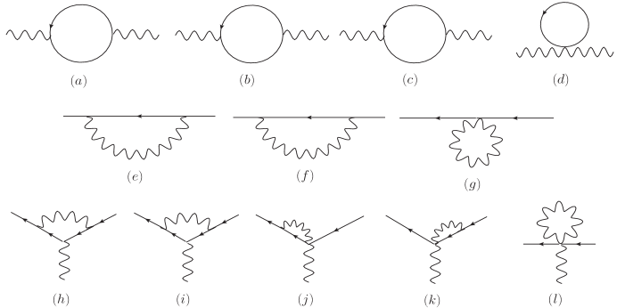
Figure 1: One-loop divergent diagrams

By weighted power counting, if diagram (a) were divergent it would produce a mass term $e^{2}\hat{A}^{2}$. However, the divergent part of diagram (a) is proportional to

$$4e^{2}\int_{-\infty}^{+\infty}\frac{\mathrm{d}\hat{p}}{2\pi}\int\frac{\mathrm{d}^{3-\varepsilon_{2}}\bar{p}}{(2\pi)^{3}}\frac{\hat{p}^{2}-b_{0}^{2}\frac{(\bar{p}^{2})^{3}}{\Lambda_{L}^{4}}}{\left(\hat{p}^{2}+b_{0}^{2}\frac{(\bar{p}^{2})^{3}}{\Lambda_{L}^{4}}+\delta^{2}\right)^{2}},$$

so it vanishes because of the identity [4]

$$\int_{-\infty}^{+\infty}\frac{\mathrm{d}\hat{p}}{2\pi}\frac{\hat{p}^{2}-x}{(\hat{p}^{\hskip 0.72229pt2}+x)^{2}}=0,\qquad x>0.$$

Diagram (b) vanishes because its integrand is odd in $\hat{p}$. All other diagrams are non-trivial.

The calculation of one-loop divergences gives the counterterms

$$\Delta_{1}\mathcal{L}_{\mathrm{E}}=\frac{\Delta_{1}\tau_{2}}{4\varepsilon_{2}}F_{\bar{\mu}\bar{\nu}}^{2}-\frac{\Delta_{1}\tau_{1}}{4\varepsilon_{2}}F_{\bar{\mu}\bar{\nu}}\frac{\bar{\partial}^{2}}{\Lambda_{L}^{2}}F_{\bar{\mu}\bar{\nu}}+\frac{1}{\varepsilon_{2}}\bar{\psi}\left(\Delta_{1}b_{1}\bar{D}\!\!\!\!/+\Delta_{1}m\right)\psi,$$

where

$$\Delta_{1}\tau_{2} = \frac{s_{0}e^{2}}{6\pi^{2}}\left(-b_{1}-4\frac{b_{0}^{\prime\prime\hskip 0.72229pt2}b_{1}}{b_{0}^{2}}-\frac{1}{2}\frac{b^{\prime\hskip 0.72229pt2}}{b_{0}}-2\frac{b_{0}^{\prime\prime\hskip 0.72229pt2}b^{\prime\hskip 0.72229pt2}}{b_{0}^{3}}-12\frac{b^{\prime}b^{\prime\prime}}{b_{0}}+8\frac{b^{\prime\prime\hskip 0.72229pt2}}{b_{0}}\right),$$

$$\Delta_{1}\tau_{1} = -\frac{e^{2}|b_{0}|}{6\pi^{2}}\left(\frac{3}{10}+2\frac{b_{0}^{\prime}}{b_{0}}-4\frac{b_{0}^{\prime\ 2}}{b_{0}^{2}}+\frac{11}{5}\frac{b_{0}^{\prime\prime\hskip 0.72229pt2}}{b_{0}^{2}}\right),$$

$$\Delta_{1}b_{1} = \frac{e^{2}}{3\pi^{2}(|b_{0}|+\sqrt{\tau_{0}})^{2}}\left(-\frac{9}{2}s_{0}b_{0}^{2}+|b_{0}|b_{0}^{\prime}-s_{0}b_{0}^{\prime\prime\hskip 0.72229pt2}+4\frac{b_{0}^{2}b_{0}^{\prime}}{\sqrt{\tau_{0}}}\right.$$

$$\left.\qquad\qquad\qquad\qquad+\frac{3}{2}\frac{b_{0}b_{0}^{\prime\hskip 0.72229pt2}}{\sqrt{\tau_{0}}}-\frac{5}{8}\frac{b_{0}b_{0}^{\prime\prime\hskip 0.72229pt2}}{\sqrt{\tau_{0}}}-\frac{7}{2}b_{0}\sqrt{\tau_{0}}-\frac{1}{2}s_{0}\tau_{0}\right),$$

$$\Delta_{1}m = \frac{e^{2}\Lambda_{L}{}}{\pi^{2}(|b_{0}|+\sqrt{\tau_{0}})}\left(-\frac{3}{4}b^{\prime}-\frac{b_{0}^{\prime\hskip 0.72229pt2}b^{\prime}}{2|b_{0}|\sqrt{\tau_{0}}}-\frac{b_{0}^{\prime\prime\hskip 0.72229pt2}b^{\prime}}{8|b_{0}|\sqrt{\tau_{0}}}+2\frac{|b_{0}|b^{\prime\prime}}{\sqrt{\tau_{0}}}+2\frac{s_{0}b_{0}^{\prime}b^{\prime\prime}}{\sqrt{\tau_{0}}}-\frac{b^{\prime}\sqrt{\tau_{0}}}{4|b_{0}|}\right),$$

and $s_{0}=b_{0}/|b_{0}|$. The fact that the sets of counterterms $\bar{\psi}\bar{\partial}\!\!\!/\psi$ and $\bar{\psi}\bar{A}\!\!\!/\psi$ combine to reconstruct the gauge-invariant expression $\bar{\psi}\bar{D}\!\!\!\!/\psi$ is a check of our results.

With respect to formulas (2.7) we have $\delta^{(1)}g_{\mathrm{R}}=(\Delta_{1}g)/\varepsilon_{2}$, where $g=\tau_{2}$, $\tau_{1}$, $b_{1}$ or $m$. Moreover, the first of (2.7) gives

$$\frac{e^{2}}{\varepsilon_{2}}=\frac{1}{\varepsilon_{2}}e_{\mathrm{B}}^{2}\mu^{-\varepsilon_{2}/3}\Lambda_{L}{}^{-2\varepsilon_{2}/3},\qquad\mu\frac{\mathrm{d}}{\mathrm{d}\mu}\left(\frac{e^{2}}{\varepsilon_{2}}\right)=-\frac{e^{2}}{3},$$

so the one-loop beta functions are

$$\beta_{g}=\frac{1}{3}\Delta_{1}g.$$

4 Relation between low-energy and high-energy divergences

In this section we study the renormalization of the low-energy theory and its relation with the renormalization of the high-energy theory.

The low-energy limit of LVQED can be studied taking the limit $\Lambda_{L}\rightarrow\infty$ in the physical correlation functions. It is described by the lagrangian

$$\mathcal{L}_{\mathrm{E}\text{{-}}\mathrm{low}}=\frac{1}{2}F_{\hat{\mu}\bar{\nu}}F_{\hat{\mu}\bar{\nu}}+\frac{\tau_{2}}{4}F_{\bar{\mu}\bar{\nu}}F_{\bar{\mu}\bar{\nu}}+\bar{\psi}\left(\hat{D}\!\!\!\!/+b_{1}\bar{D}\!\!\!\!/+m\right)\psi,$$ (4.1)

(in Euclidean space). We refer to this theory as lvQED. The low-energy values of $\tau_{2}$ and $b_{1}$ have to be sufficiently close to 1 to have agreement with experiments (see [1]). Here, however, we are interested in more theoretical aspects. Our goal is to compare the renormalizations of LVQED and lvQED, and explain in detail how the high-energy divergences in $1/\varepsilon_{2}$ combine with the $\Lambda_{L}$-divergences to reproduce the low-energy results. We discover that the low-energy power-like divergences are multiplied by arbitrary constants, inherited by the high-energy theory. This makes the hierarchy problem disappear.

Let us call the theory (2), equipped with its dimensional-regularization technique, LVQED_ε. From the low-energy point of view, LVQED_ε can be viewed as a particular regularization of (4.1) with a combination of two cut-offs: the dimensional one and $\Lambda_{L}$.

Specifically, if $\Lambda_{L}$ is viewed as a cut-off, (2) can be understood as a (partial) regularization of (4.1). The regularization is then completed dimensionally continuing the space dimensions to $3-\varepsilon_{2}$, with the prescription that the limit $\varepsilon_{2}\rightarrow 0$ be taken before the limit $\Lambda_{L}\rightarrow\infty$.

Recall that when two or more cut-offs are used to regularize a theory they can be removed in any preferred order, up to a change of scheme. In a single one-loop integral, the result can change at most by local terms, which are possibly divergent. In higher-loop integrals the same conclusion holds when the subdivergences are removed by appropriate counterterms. If we consider not just isolated integrals, but the procedure of regularization and subtraction of counterterms as a whole, the limit-interchange can generate results that differ at most by finite local terms, which is precisely a scheme change. Once physical normalization conditions are imposed, all physical quantities coincide.

Moreover, two cut-offs can be identified only up to an arbitrary constant. For example, we have

$$\frac{1}{\varepsilon_{2}}=\ln\Lambda_{L}+c,$$ (4.2)

and the constant $c$ has no universal meaning. We can even choose different constants $c$ for each high-energy divergence. Indeed, changing $c$ to $c+\delta c$ amounts to shift the pole subtraction from $1/\varepsilon_{2}$ to $1/\varepsilon_{2}-\delta c$ in the high-energy theory. Details about cut-off identifications are given in Appendix B.

Summarizing, an equivalent regularization of (4.1) can be obtained from LVQED_ε, where however the limit $\Lambda_{L}\rightarrow\infty$ is taken before the limit $\varepsilon_{2}\rightarrow 0$. When $\Lambda_{L}$ goes to infinity (2) just collapses to (4.1). Since $\varepsilon_{2}$ is still non-vanishing, we just obtain lvQED_ε, namely a dimensional regularization of (4.1), where only space is continued to complex dimensions.

Now, one-loop logarithmic divergences are scheme independent, so they can be calculated removing the two cut-offs in either order. On the other hand, power-like divergences do depend on the scheme. Since we regard LVQED as a fundamental theory, not just a partial regularization of (4.1), the powers of $\Lambda_{L}$ must be studied taking $\varepsilon_{2}\rightarrow 0$ first.

It turns out that the power-like divergences in $\Lambda_{L}$ are multiplied by arbitrary incalculable constants, inherited by the scheme arbitrariness of the high-energy theory. Thus, they are devoid of any physical meaning. Ultimately, we discover that it is completely safe to study the low-energy theory sending $\Lambda_{L}$ to infinity at $\varepsilon_{2}\neq 0$.

In the rest of this section we perform a detailed analysis and prove these statements. A one-loop correlation function is the sum of contributions of the form $I_{r}/\Lambda_{L}^{r}$, where $r$ is a non-negative integer and

$$I_{r}=\int\frac{\mathrm{d}\hat{p}\ \mathrm{d}^{3-\varepsilon_{2}}\bar{p}}{(2\pi)^{4}}\frac{N_{s}(\hat{p},\bar{p},\hat{k},\bar{k})}{\prod_{i=1}^{n}\left[(\hat{p}-\hat{k}_{i})^{2}+a_{i}(\bar{p}-\bar{k}_{i})^{2}+m_{i}^{2}+(\bar{p}-\bar{k}_{i})^{2}\Delta_{i}((\bar{p}-\bar{k}_{i})^{2}/\Lambda_{L}^{2})\right]},$$ (4.3)

where $\Delta_{i}(x)$ are some polynomials such that $\Delta_{i}(0)=0$ and the $k_{i}$’s denote linear combinations of the external momenta $k$. The numerator $N_{s}$ is a certain monomial of degree $s$ in momenta. Below we prove that the integral $I_{r}$ is equivalent to

$$I_{r<}^{\prime}=\int_{|\bar{p}|\leqslant\Lambda_{L}}\frac{\mathrm{d}\hat{p}\ \mathrm{d}^{3}\bar{p}}{(2\pi)^{4}}\frac{N_{s}(\hat{p},\bar{p},\hat{k},\bar{k})}{\prod_{i=1}^{n}\left[(\hat{p}-\hat{k}_{i})^{2}+a_{i}(\bar{p}-\bar{k}_{i})^{2}+m_{i}^{2}\right]},$$ (4.4)

up to a scheme change, namely up to local counterterms that are at most power-like divergent. Thus, $I_{r}/\Lambda_{L}^{r}$ is also equivalent to $I_{r<}^{\prime}/\Lambda_{L}^{r}$ up to a scheme change. Now, since $I_{r<}^{\prime}$ is a one-loop integral, its divergences can only be powers or logarithms (but not powers times logarithms). By the locality of counterterms, $I_{r<}^{\prime}$ has the form

$$I_{r<}^{\prime}=P(\Lambda_{L},m,k)+P^{\prime}(m,k)\ln\Lambda_{L}+\mathrm{finite}+\mathcal{O}(1/\Lambda_{L}),$$

where $P$ and $P^{\prime}$ are polynomials. Thus, whenever $r>0$, the contribution of $I_{r<}^{\prime}/\Lambda_{L}^{r}$ (and $I_{r}/\Lambda_{L}^{r}$) is just a scheme change. Only the contributions with $r=0$ determine the physical quantities. However, the integrals $I_{0<}^{\prime}$ are precisely those of the low-energy theory regulated with the cut-off $\Lambda_{L}$. This proves that the low-energy limit of LVQED can be studied, up to a scheme change, regulating (4.1) with a cut-off $\Lambda_{L}$ on the space momenta.

In particular, the scheme-independent contributions to the low-energy renormalization of LVQED are encoded in $I_{0<}^{\prime}$. Instead, the scheme-dependent quantities have to be studied directly on LVQED.

The next goal is to prove the equivalence of (4.3) and (4.4) up to a scheme change. As a byproduct, it emerges that the low-energy power-like divergences are multiplied by arbitrary constants. Before treating the general case, we illustrate a simple example.

Illustrative example

Consider the tadpole integral

$$I=\int\frac{\mathrm{d}\hat{p}\ \mathrm{d}^{3-\varepsilon_{2}}\bar{p}}{(2\pi)^{4}}\frac{1}{D(\hat{p},\bar{p},m)+\bar{p}^{2}\Delta(\bar{p}^{2}/\Lambda_{L}^{2})},$$

where

$$D(\hat{p},\bar{p},m)=\hat{p}^{2}+a_{2}\bar{p}^{2}+m^{2},\qquad\Delta(x)=a_{0}x^{2}+a_{1}x,$$

and $a_{0},a_{2}>0$. At $\Lambda_{L}$ finite, this integral is logarithmically divergent. When $\Lambda_{L}\rightarrow\infty$ , it becomes quadratically divergent.

It is convenient to split the $\bar{p}$-domain of integration in two regions: the sphere $|\bar{p}|\leqslant\Lambda_{L}$ and the crown $|\bar{p}|\geqslant\Lambda_{L}$. Rescaling $\hat{p},\bar{p}$ to $\Lambda_{L}\hat{p},\Lambda_{L}\bar{p}$ we get

$$I=I_{<}+I_{>},\qquad I_{\lessgtr}=\Lambda_{L}^{2-\varepsilon_{2}}\int_{|\bar{p}|\lessgtr 1}\frac{\mathrm{d}\hat{p}\ \mathrm{d}^{3-\varepsilon_{2}}\bar{p}}{(2\pi)^{4}}\frac{1}{D(\hat{p},\bar{p},m/\Lambda_{L})+\bar{p}^{2}\Delta(\bar{p}^{2})}.$$

We want to show that $I$ is equivalent to

$$I_{<}^{\prime}=\int_{|\bar{p}|\leqslant\Lambda_{L}}\frac{\mathrm{d}\hat{p}\ \mathrm{d}^{3}\bar{p}}{(2\pi)^{4}}\frac{1}{D(\hat{p},\bar{p},m)}=\Lambda_{L}^{2}\int_{|\bar{p}|\leqslant 1}\frac{\mathrm{d}\hat{p}\ \mathrm{d}^{3}\bar{p}}{(2\pi)^{4}}\frac{1}{D(\hat{p},\bar{p},m/\Lambda_{L})},$$

up to a scheme change.

Consider first $I_{>}$. The integrand can be expanded in powers of $m$ (there are no infrared problems, since $\bar{p}$ cannot approach zero). We can write

$$I_{>}=\sum_{k=0}^{\infty}(-1)^{k}\Lambda_{L}^{2-\varepsilon_{2}-2k}m^{2k}I_{k},\qquad I_{k}=\int_{|\bar{p}|>1}\frac{\mathrm{d}\hat{p}\ \mathrm{d}^{3-\varepsilon_{2}}\bar{p}}{(2\pi)^{4}}\frac{1}{\mathcal{D}^{k+1}(\hat{p},\bar{p},0)}.$$

where

$$\mathcal{D}(\hat{p},\bar{p},0)\equiv D(\hat{p},\bar{p},0)+\bar{p}^{2}\Delta(\bar{p}^{2}).$$

When $\varepsilon_{2}\rightarrow 0$ only $I_{0}$ diverges. Let us write

$$I_{0}=\frac{A_{0}}{\varepsilon_{2}}+B_{0}+\mathcal{O}(\varepsilon_{2}),\qquad I_{k}=B_{k}+\mathcal{O}(\varepsilon_{2})\quad\mathrm{{\ for}\,}k\mathrm{>0,}$$

where $A_{i},B_{i}$ are constants. We have, for $\varepsilon_{2}\sim 0$,

$$I_{>}=\Lambda_{L}^{2}\left[A_{0}\left(\frac{1}{\varepsilon_{2}}-\ln\Lambda_{L}\right)+B_{0}\right]-B_{1}m^{2}+\mathcal{O}(\varepsilon_{2},m^{2}/\Lambda_{L}^{2}).$$

To translate this expression into more familiar terms, just recall that if we had regulated the high-energy theory with a cut-off $\Lambda$ instead of using the dimensional regularization, the coefficient of $A_{0}$ between the square brackets would be ln$(\Lambda/\Lambda_{L})$.

Taking $\Lambda_{L}\rightarrow\infty$ after $\varepsilon_{2}\rightarrow 0$ we thus find, using (4.2),

$$I_{>}\rightarrow\Lambda_{L}^{2}(cA_{0}+B_{0})-B_{1}m^{2}.$$

We see that the contribution of the crown does not contain logarithmic divergences and it is polynomial in the mass. Moreover, the coefficients of the power-like divergences remain undetermined.

Now, let us study $I_{<}$. Here we can immediately take the limit $\varepsilon_{2}\rightarrow 0$, since the integral is UV convergent. Define $X$ so that

$$I_{<}=I_{<}^{\prime}+\Lambda_{L}^{2}J+m^{2}X,$$

where

$$J=-\int_{|\bar{p}|\leqslant 1}\frac{\mathrm{d}\hat{p}\ \mathrm{d}^{3}\bar{p}}{(2\pi)^{4}}\frac{\bar{p}^{2}\Delta(\bar{p}^{2})}{D(\hat{p},\bar{p},0)\mathcal{D}(\hat{p},\bar{p},0)}<\infty.$$ (4.5)

It is easy to see that $X$ is regular in the limit $\Lambda_{L}\rightarrow\infty$. Its limit $\bar{X}$ reads

$$\bar{X}=\int_{|\bar{p}|\leqslant 1}\frac{\mathrm{d}\hat{p}\ \mathrm{d}^{3}\bar{p}}{(2\pi)^{4}}\frac{\bar{p}^{2}\Delta(\bar{p}^{2})\left(D(\hat{p},\bar{p},0)+\mathcal{D}(\hat{p},\bar{p},0)\right)}{D^{2}(\hat{p},\bar{p},0)\mathcal{D}^{2}(\hat{p},\bar{p},0)}<\infty.$$

Here and in (4.5) it is crucial to check the absence of infrared divergences at $p\sim 0$.

Calculating $I_{<}^{\prime}$ and collecting our results, we get

$$I=\Lambda_{L}^{2}\left(\frac{1}{8\pi^{2}a_{2}^{1/2}}+cA_{0}+B_{0}+J\right)-m^{2}\left(\frac{\ln(4a_{2}\Lambda_{L}^{2}/m^{2})-1}{16\pi^{2}a_{2}^{3/2}}+B_{1}-\bar{X}\right)+\mathcal{O}(m^{2}/\Lambda_{L}^{2}).$$ (4.6)

Thus, the scheme-independent divergences are contained in $I_{<}^{\prime}$. The quadratic divergences remain arbitrary, due to the constant $c$ inherited from the high-energy theory.

Observe that another argument to justify the identification (4.2) is that $I$ cannot have divergences of the form $\Lambda_{L}^{2}/\varepsilon_{2}$ or $\Lambda_{L}^{2}\ln\Lambda_{L}$, because they can arise only at higher loops.

General case

Now we give the general argument for the equivalence of (4.3) and (4.4) up to a scheme change. The degree of divergence $\omega$ of $I_{r<}^{\prime}$ is $s+4-2n$. If $\omega<0$ the limits $\varepsilon_{2}\rightarrow 0$ and $\Lambda_{L}\rightarrow\infty$ can be taken directly on the integrand of $I_{r}$ and the result is equal to the limit $\Lambda_{L}\rightarrow\infty$ of $I_{r<}^{\prime}$, which is finite. Thus, we can assume $\omega\geqslant 0$.

Again, split the $\bar{p}$-domain of integration in two regions: the sphere $|\bar{p}|\leqslant\Lambda_{L}$ and the crown $|\bar{p}|\geqslant\Lambda_{L}$, and call $I_{r>}$ and $I_{r<}$ the two contributions to $I_{r}$. Rescaling $\hat{p},\bar{p}$ to $\Lambda_{L}\hat{p},\Lambda_{L}\bar{p}$, we get

$$I_{r>}=\Lambda_{L}^{\omega-\varepsilon_{2}}\int_{|\bar{p}|\geqslant 1}\frac{\mathrm{d}\hat{p}\ \mathrm{d}^{3-\varepsilon_{2}}\bar{p}}{(2\pi)^{4}}\frac{N_{s}(\hat{p},\bar{p},\hat{k}/\Lambda_{L},\bar{k}/\Lambda_{L})}{\prod_{i=1}^{n}\mathcal{D}_{i}(\hat{p}-\hat{k}_{i}/\Lambda_{L},\bar{p}-\bar{k}_{i}/\Lambda_{L},m_{i}/\Lambda_{L})},$$ (4.7)

where

$$\mathcal{D}_{i}(\hat{p},\bar{p},m_{i})=\hat{p}^{2}+a_{i}\bar{p}^{2}+m_{i}^{2}+\bar{p}^{2}\Delta_{i}(\bar{p}^{2}).$$

Now, expand the expression (4.7) in powers of $k/\Lambda_{L}$ and $m/\Lambda_{L}$, which is allowed because the integral has an IR cut-off. After a finite number of terms we get contributions that are finite for $\varepsilon_{2}\rightarrow 0$ and disappear when later $\Lambda_{L}\rightarrow\infty$. Thus the result of these limits on $I_{r>}$ is a polynomial in $k$ and $m$. The coefficients are powers $\Lambda_{L}^{i}$, possibly multiplied by simple poles $1/\varepsilon_{2}$. Since

$$\frac{\Lambda_{L}^{i-\varepsilon_{2}}}{\varepsilon_{2}}=\Lambda_{L}^{i}\left(\frac{1}{\varepsilon_{2}}-\ln\Lambda_{L}+\mathcal{O}(\varepsilon_{2})\right)\rightarrow\Lambda_{L}^{i}\left(c_{i}+\mathcal{O}(\varepsilon_{2})\right),$$

we see that all power-like divergences are multiplied by (different) arbitrary constants $c_{i}$ and no $\ln\Lambda_{L}$ can appear.

Next, consider $I_{r<}-I_{r<}^{\prime}$. We can set $\varepsilon_{2}=0$, since there are no ultraviolet divergences here. To keep the notation simple, let us collect both $k$’s and $m$’s in the same symbol $K$ and leave index contractions implicit. Define $K^{\omega}X$ as the difference between $I_{r<}-I_{r<}^{\prime}$ and its expansion in $k/\Lambda_{L}$ and $m/\Lambda_{L}$ up to the order $\omega-1$. We have

$$I_{r<}=I_{r<}^{\prime}+\sum_{i=0}^{\omega-1}\Lambda_{L}^{\omega-i}K^{i}J_{i}+K^{\omega}X.$$

Now, by construction all $J_{i}$’s are integrals of functions depending only on $\hat{p}$ and $\bar{p}$ and no other dimensionful quantities. Such integrals have a UV cut-off ($|\bar{p}|\leqslant 1$). Moreover, power counting shows that they are also IR convergent, because they have dimensions $\omega-i$. Next, we need to check that the $\Lambda_{L}\rightarrow\infty$ (or $K\rightarrow 0$) limit $\bar{X}$ of $X$ is well defined. Again, there are no UV problems, but we must check IR convergence. Although $X$ has dimension zero, we must recall that it is originated expanding the difference $I_{r<}-I_{r<}^{\prime}$, whose integrand is proportional to a polynomial $\Delta(x)=\mathcal{O}(x)$. The factor $\Delta$ enhances the naive IR power counting by two units, just enough to make $\bar{X}$ well defined.

This concludes the proof.

5 Low-energy counterterms

In this section we compute the renormalization of lvQED. Using the results of the previous section, we know that we do not need to pay attention to power-like divergences, so we just focus on the logarithmic ones. The contributing diagrams are (a), (b), (c), (e), (f), (h) and (i), plus the same as (h) and (i) but with $\hat{A}$-external legs. The key-integrals are collected in appendix A. We find

$$\frac{\Delta_{1}\mathcal{L}_{\mathrm{E}\text{{-}}\mathrm{low}}}{\ln(\Lambda_{L}/\mu)} = -\frac{e^{2}}{6\pi^{2}|b_{1}|}\left(\frac{1}{2}F_{\hat{\mu}\bar{\nu}}F_{\hat{\mu}\bar{\nu}}+\frac{b_{1}^{2}}{4}F_{\bar{\mu}\bar{\nu}}F_{\bar{\mu}\bar{\nu}}\right)-\frac{e^{2}(\tau_{2}+3b_{1}^{2})}{4\pi^{2}|b_{1}|\sqrt{\tau_{2}}(|b_{1}|+\sqrt{\tau_{2}})}m\bar{\psi}\psi$$ (5.2)

$$+\frac{e^{2}(\tau_{2}-3b_{1}^{2})}{4\pi^{2}\sqrt{\tau_{2}}(|b_{1}|+\sqrt{\tau_{2}})^{2}}\bar{\psi}\hat{D}\!\!\!\!/\psi-\frac{e^{2}(\tau_{2}+b_{1}^{2})(|b_{1}|+2\sqrt{\tau_{2}})}{12\pi^{2}|b_{1}|\sqrt{\tau_{2}}(|b_{1}|+\sqrt{\tau_{2}})^{2}}b_{1}\bar{\psi}\bar{D}\!\!\!\!/\psi.$$

Thus,

$$\beta_{e} = e\gamma_{A}=\frac{e^{3}}{12\pi^{2}|b_{1}|},\qquad\beta_{\tau_{2}}=\frac{e^{2}(\tau_{2}-b_{1}^{2})}{6\pi^{2}|b_{1}|},\qquad\beta_{b_{1}}=-\frac{e^{2}b_{1}\left(2|b_{1}|(\tau_{2}-2b_{1}^{2})+\sqrt{\tau_{2}}(\tau_{2}+b_{1}^{2})\right)}{6\pi^{2}|b_{1}|\sqrt{\tau_{2}}(|b_{1}|+\sqrt{\tau_{2}})^{2}},$$

$$\gamma_{\psi} = -\frac{e^{2}(\tau_{2}-3b_{1}^{2})}{8\pi^{2}\sqrt{\tau_{2}}(|b_{1}|+\sqrt{\tau_{2}})^{2}},\qquad\beta_{m}=-m\frac{e^{2}(2|b_{1}|\sqrt{\tau_{2}}+\tau_{2}+3b_{1}^{2})}{4\pi^{2}|b_{1}|(|b_{1}|+\sqrt{\tau_{2}})^{2}}.$$

Around the Lorentz invariant surface our results agree with those found by Kostelecky, Lane and Pickering [9], once restricted to the CPT-, P- and rotation invariant case. See also the more recent paper [10]. Another check of our results is that setting

$$\tau_{2}=b_{1}^{2},$$ (5.3)

we recover QED. Indeed, when (5.3) holds, then both $\tau_{2}$ and $b_{1}$ can be set to 1 rescaling the space coordinates (as well as the fields and $e$). Then $\beta_{\tau_{2}}$ and $\beta_{b_{1}}$ vanish, while $\beta_{e}$, $\gamma_{\psi}$ and $\beta_{m}$ take their known values.

6 The new setting of the hierarchy problem

In the previous section we have seen that at low energies the power-like divergences in $\Lambda_{L}$ are multiplied by arbitrary constants, the arbitrariness being inherited by the divergences of the high-energy theory. Those arguments are very general, in particular they also apply to the Lorentz violating Standard Models of [3, 4]. These facts force us to reconsider the hierarchy problem. For definiteness, we treat the Higgs mass.

In general, when new physics beyond the Standard Model is assumed, it is assumed to be described by a finite theory, that contains a physical energy scale $\Lambda$ and gives the Standard Model when $\Lambda$ is sent to infinity. Then, at energies much smaller than $\Lambda$ the Higgs mass is corrected by physical quadratic divergences, and their removal poses a fine-tuning problem. On the other hand, if the Standard Model were exact at arbitrarily high-energies, the quadratic divergences of the Higgs mass would have no physical meaning (among the other things, they would be scheme-dependent) and could be removed with a mathematical operation devoid of physical significance.

Our extensions of the Standard Model model do assume new physics beyond the Standard Model, but not described by a finite theory, rather a super-renormalizable one. Our results show that the coefficient of the quadratic divergences is still scheme-dependent and devoid of physical meaning. In this section we explain that, because of this, no fine-tuning problem arises. We stress that our statement does not contraddict the common lore about the hierarchy problem, because our models do not obey the finiteness assumption.

The general form of the (one-loop) mass renormalization can be read for example from (4.6). We have

$$m_{\Lambda}^{2}=m^{2}+a\Lambda_{L}^{2}\ln\frac{\Lambda^{2}}{\Lambda_{L}^{2}}+bm^{2}\ln\frac{\Lambda_{L}^{2}}{m^{2}}+c\Lambda_{L}^{2}+dm^{2}.$$ (6.1)

Here $m_{\Lambda}$ denotes the bare mass, $m$ is the low-energy mass, $\Lambda$ is the ultraviolet cut-off (we have replaced $1/\varepsilon_{2}$ with $\ln\Lambda+$constant), while $a$, $b$ and $d$ are calculable coefficients, depending on the parameters of the theory. In LVQED the formula of the electron-mass renormalization has a form analogous to (6.1), but the squares $m_{\Lambda}^{2}$, $m^{2}$, $\Lambda^{2}$ and $\Lambda_{L}^{2}$ are replaced by $m_{\Lambda}$, $m$, $\Lambda$ and $\Lambda_{L}$, respectively, and the coefficient $a$ can be read from (3).

If $\Lambda$ were the physical scale introduced by a finite ultraviolet completion of the theory, $c$ would also be calculable. Then we would have a fine-tuning problem: roughly, $m^{2}$ is small and $a\Lambda_{L}^{2}\ln(\Lambda^{2}/\Lambda_{L}^{2})$ is large, so $m_{\Lambda}^{2}$ is also large and

$$m^{2}=\text{small}=\text{large}-\text{large.}$$

On the other hand, if our models are regarded as fundamental models of the Universe (when gravity is switched off), namely if we assume that no more fundamental models exist beyond them, then $\Lambda$ is an unphysical cut-off, which means that it must be sent to infinity, and $c$ remains scheme-dependent, therefore arbitrary. Then, both $a\Lambda_{L}^{2}\ln(\Lambda^{2}/\Lambda_{L}^{2})$ and $m_{\Lambda}^{2}$ are infinite, so

$$m^{2}=\infty-\infty.$$

This cancellation between infinities is just the usual job of renormalization. There is no fine-tuning problem, because $m^{2}$ cannot be said to be small or large with respect to infinity.

We can make this even clearer eliminating the cut-off $\Lambda$. Formula (6.1) incorporates also the (one-loop) running from energies $\Lambda$ to energies $\Lambda_{L}$. In other words, if we substitute $\Lambda$ with $\Lambda_{L}$ formula (6.1) gives an expression for the Higgs mass $m_{L}$ at the scale of Lorentz violation. We find

$$m_{L}^{2}=m^{2}+bm^{2}\ln\frac{\Lambda_{L}^{2}}{m^{2}}+c\Lambda_{L}^{2}+dm^{2}.$$

We see that the quadratic divergence $\sim\Lambda_{L}^{2}$ is still multiplied by the meaningless arbitrary constant $c$, which cannot be eliminated. There is no reason why the quantity $c\Lambda_{L}^{2}$ should be large, even if $\Lambda_{L}^{2}$ is large. Actually, we can use the arbitrariness of $c$ to make it disappear, and obtain

$$m_{L}^{2}=m^{2}+bm^{2}\ln\frac{\Lambda_{L}^{2}}{m^{2}}+dm^{2}.$$

Again, we do not find any fine-tuning problem.

Our argument is very general. It does not depend on the particular high-energy completion of the theory, as long as it is not finite. Indeed, if the UV completion is not finite, at some point we do need an unphysical cut-off $\Lambda$, which brings some arbitrariness into the game and makes the quadratic divergences unphysical.

In conclusion, the hierarchy problem is a true problem only if the ultimate theory of the Universe is completely finite. If the ultimate theory of the Universe is just renormalizable, or even super-renormalizable, for example one of the models that we propose, then the hierarchy problem disappears.

7 Conclusions

In this paper we have studied the one-loop renormalization of high-energy Lorentz violating QED, a subsector of the Lorentz violating Extended Standard Model proposed recently. We have also analyzed the interplay between high-energy and low-energy renormalizations in detail.

We have shown that the high-energy theory leaves important remnants at low energies, such as incalculable, arbitrary factors in front of all power-like divergences. This property holds under the sole assumption that the fundamental theory beyond the Standard Model, whether it is (1.1) or not, is not completely finite, but just renormalizable, or even super-renormalizable. In particular, the arbitrariness inherited by the high-energy theory allows us to eliminate the quadratically divergent corrections to the Higgs mass, thereby removing the hierarchy problem.

Acknowledgments

One of us (D.A.) is grateful to D. Buttazzo for useful discussions.

Appendix A: Key integrals

For the calculations of the high-energy renormalization we just need the divergent part of one integral, namely

$$\int\frac{\mathrm{d}\hat{p}\ \mathrm{d}^{3-\varepsilon_{2}}\bar{p}}{(2\pi)^{4}}\frac{\hat{p}^{q}(\bar{p}^{2})^{r}(\bar{p}\cdot\bar{k})^{s}}{\left(\hat{p}^{2}+b_{0}^{2}\frac{(\bar{p}^{2})^{3}}{\Lambda_{L}^{4}}+\delta^{2}\right)^{k_{1}}\left(\hat{p}^{2}+\tau_{0}\frac{(\bar{p}^{2})^{3}}{\Lambda_{L}^{4}}+\delta^{2}\right)^{k_{2}}},$$

for $2+q+(s+2r)/3=2(k_{1}+k_{2})$. Using Feynman parameters we can immediately integrate over $\hat{p}$. This isolates the pole of the $\bar{p}$-integral, therefore the divergent part. The remaining integral over the Feynman parameter gives a hypergeometric function. The final result is

$$\frac{\tau_{0}^{(1+q)/2-k_{1}-k_{2}}}{\Lambda_{L}^{2+2q-4k_{1}-4k_{2}}}\frac{(\bar{k}^{2})^{s/2}}{\varepsilon_{2}}\frac{\left(1+(-1)^{s}\right)\left(1+(-1)^{q}\right)\Gamma\left(\frac{q+1}{2}\right)\Gamma\left(k_{1}+k_{2}-\frac{q+1}{2}\right)}{2(s+1)(2\pi)^{3}\Gamma(k_{1}+k_{2})}\times$$

$$\qquad\qquad\qquad\times\ _{2}F_{1}\left(k_{1},k_{1}+k_{2}-\frac{q+1}{2},k_{1}+k_{2},1-\frac{b_{0}^{2}}{\tau_{0}}\right).$$

For the calculations of the low-energy renormalization we need the logarithmic divergences of two integrals, namely

$$\int_{|\bar{p}|\leqslant\Lambda_{L}}\frac{\mathrm{d}\hat{p}\ \mathrm{d}^{3}\bar{p}}{(2\pi)^{4}}\frac{(\hat{p}^{2},\bar{p}^{2})}{\left(\hat{p}^{2}+b_{1}^{2}\bar{p}^{2}+m^{2}\right)^{2}\left(\hat{p}^{2}+\tau_{2}\bar{p}^{2}\right)}\sim\frac{\ln(\Lambda_{L}/m)}{8\pi^{2}|b_{1}|(|b_{1}|+\sqrt{\tau_{2}})^{2}}\left(1,\frac{2|b_{1}|+\sqrt{\tau_{2}}}{b_{1}^{2}\sqrt{\tau_{2}}}\right).$$ (A.1)

As usual, the one-loop calculation is done expanding in external momenta. This gives a sum of contributions involving the integrals (A.1), plus more standard integrals and integrals that do not have logarithmic divergences.

Appendix B: Identification of cut-offs

Formula (4.2) can be proved comparing two different regularizations of the same integral. The first technique is a dimensional regularization where only the space dimension is continued to complex values. The second technique is a higher-derivative regularization where only higher-space derivatives are used. We get

$$\int\frac{\mathrm{d}\hat{p}\ \mathrm{d}^{3-\varepsilon_{2}}\bar{p}}{(2\pi)^{4}}\frac{1}{(\hat{p}^{2}+\bar{p}^{2}+m^{2})^{2}} = \frac{2}{(4\pi)^{2}\varepsilon_{2}}+\mathrm{constant,}$$

$$\int\frac{\mathrm{d}\hat{p}\ \mathrm{d}^{3}\bar{p}}{(2\pi)^{4}}\frac{1}{\left(\hat{p}^{2}+\bar{p}^{2}+m^{2}+\frac{(\bar{p}^{2}+m^{2})^{2}}{\Lambda_{L}^{2}}\right)^{2}} = \frac{\ln(\Lambda_{L}/m)}{8\pi^{2}}+\mathrm{constant,}$$

whence (4.2) follows. Similarly, if we use a cut-off on the $\bar{p}$-integral instead of higher-space derivatives, we get

$$\int_{|\bar{p}|\leqslant\Lambda_{L}}\frac{\mathrm{d}\hat{p}\ \mathrm{d}^{3}\bar{p}}{(2\pi)^{4}}\frac{1}{\left(\hat{p}^{2}+\bar{p}^{2}+m^{2}\right)^{2}}=\frac{\ln(\Lambda_{L}/m)}{8\pi^{2}}+\mathrm{constant.}$$

References

• [1] V.A. Kostelecký and N. Russell, Data tables for Lorentz and CTP violation, V.A. Kostelecký, Ed., Proceedings of the Fourth Meeting on CPT and Lorentz Symmetry, World Scientific, Singapore, 2008, p. 308 and arXiv:0801.0287 [hep-ph].
• [2] D. Anselmi and M. Halat, Renormalization of Lorentz violating theories, Phys. Rev. D 76 (2007) 125011 and arXiv:0707.2480 [hep-th].
• [3] D. Anselmi, Weighted power counting, neutrino masses and Lorentz violating extensions of the Standard Model, Phys. Rev. D 79 (2009) 025017 and arXiv:0808.3475 [hep-ph].
• [4] D. Anselmi, Standard Model Without Elementary Scalars And High Energy Lorentz Violation, Eur. Phys. J. C 65 (2010) 523 and arXiv:0904.1849 [hep-ph].
• [5] D. Anselmi, Weighted scale invariant quantum field theories, JHEP 02 (2008) 051 and arXiv:0801.1216 [hep-th].
• [6] N.N. Bogoliubov and D.V. Shirkov, Introduction to the theory of quantized fields, Interscience Publishers, New York, 1959, §17.5, formula (17.30);
• [7] G. ’t Hooft and M. Veltman, Diagrammar, report CERN-73-09, available at http://cdsweb.cern.ch/record/186259, §6.4, formula (6.19).
• [8] T.D. Bakeyev and A.A. Slavnov, Higher covariant derivative regularization revisited, Mod. Phys. Lett. A11 (1996) 1539 and arXiv:hep-th/9601092, and references therein.
• [9] V.A. Kostelecky, C. Lane and A. Pickering, One-loop renormalization of Lorentz-violating electrodynamics, Phys. Rev. D. 65 (2002) 056006 and arXiv:hep-th/0111123.
• [10] D. Colladay and P. McDonald, One-loop renormalization of the electroweak sector with Lorentz violation, Phys. Rev. D 79 (2009) 125019 and arXiv:0904.1219 [hep-ph].