Casimir interactions in Ising strips with boundary fields: exact results.

Abstract

An exact statistical mechanical derivation is given of the critical Casimir forces for Ising strips with arbitrary surface fields applied to edges. Our results show that the strength as well as the sign of the force can be controled by varying the temperature or the fields. An interpretation of the results is given in terms of a linked cluster expansion. This suggests a systematic approach for deriving the critical Casimir force which can be used in more general models.

Casimir forces Casimir arise in the quantum electrodynamics of geometrically restricted systems, for instance between two metal plates in vacuo, because the photon spectrum is modified; typically the force is attractive. Fisher and de Gennes FdG proposed that analogous Casimir forces should arise in condensed matter systems near a second-order phase transition, the agent being thermally-excited fluctuations of the order parameter, e.g. of the density, rather then of the photon field. Of particular interest, both experimental and theoretical, is their scaling-theoretic prediction that such interactions should have a power law dependence on distance in the critical scaling region. For example, in spatial dimension $d$ for walls separated by a distance $N$, the Casimir force per unit area is ${\cal F}_{Cas}=-N^{-d}\vartheta(N/\xi)$, where $\xi$ is the bulk correlation length FdG ; krech:99:0 ; Dbook . (All free energies and forces are expressed in units of $k_{B}T$.) The tunability of critical Casimir interactions will be crucial for many applications in micro and nano systems, e.g. in colloids or in various micro or nano-electromechanical devices, in particular, to be able to produce repulsive interactions to counteract the omnipresent attractive Casimir quantum electrodynamical force.

If the system is confined to a film, one would expect on intuitive grounds that the geometrical effect on the order parameter fluctuations of the strip boundaries, would be to reduce the entropy; thereby establishing a strictly repulsive force. This argument is incomplete because some energetic factors are neglected. We propose an alternative view that admits attractive forces. Let us examine the following approximate treatment of a $2d$ Ising strip of finite width $N$ and with free boundaries. Following Privman and Fisher privman , the low energy excitation of such a model are domain walls, each with free energy $N\tau$ where $\tau$ is the incremental free energy per unit length for an interface perpendicular to the strip axis. A collection of these is then treated as a $1d$ Ising model with cyclic boundary conditions. A simple calculation shows that the limiting incremental free energy, per unit length of strip, is $f^{\times}=-\log\left(1+e^{-N\tau}\right)$ and then the Casimir force, again per unit length, is ${\cal F}_{Cas}=-\partial f^{\times}/\partial N=-\tau/(e^{N\tau}+1).$ In the scaling limit $N\tau=x,N\to\infty,\tau\to 0$, (1) becomes

$$N{\cal F}_{Cas}(x)\rightarrow-\frac{x}{e^{x}+1}.$$ (1)

Notice that this force is attractive, but the power of $N$ disagrees with FdG . What is missing in this formula? Firstly, there is no mention of any thermally-excited intrinsic structure of the individual domain walls. This could perhaps be included for the planar Ising model with free boundaries by calculating the partition function of a single interface connecting the edges with one end fixed, but the other free; this merely reproduces (1). Secondly, the detailed interactions of these domain walls must be quite complicated, but they are evidently accounted for in exact calculations on planar Ising strips. The first known results ES were for the strip with zero bulk field and either free boundary condition or fixed boundary spins, both the $++$ and $+-$ conditions.

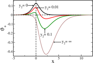
Figure 1: (color online) The scaling function $\vartheta_{+}(x,y_{1},y_{2})$ of the critical Casimir force (7) for the isotropic lattice with $K_{1}=K_{2}$, $y_{1}=h_{1}^{2}N=\infty$ and for the several values of $y_{2}=h_{2}^{2}N$.

The partition function for the free strip is DBMIT

$$Z_{f}=\prod_{\begin{subarray}{c}0<\omega\leq\pi\\ e^{iN\omega}=-1\end{subarray}}\left[\cosh N\gamma(\omega)+\sinh N\gamma(\omega)\cos\delta^{\prime}(\omega)\right].$$ (2)

The Onsager functions onsager $\gamma(\omega)$ and $\delta^{\prime}(\omega)$ are given by $\cosh\gamma(\omega)=\cosh 2K_{2}\cosh 2K_{1}^{*}-\sinh 2K_{2}\sinh 2K_{1}^{*}\cos\omega$, and

$$e^{i\delta^{\prime}(\omega)}=\left[\left(z-A\right)\left(z-B\right)/\left(Az-1\right)\left(Bz-1\right)\right]^{1/2}.$$ (3)

where $z=e^{i\omega}$, $A=\exp 2(K_{1}+K_{2}^{*})$ and $B=\exp 2(K_{1}-K_{2}^{*})$. $K_{1}$ and $K_{2}$ are the nearest neighbour couplings (in units of $k_{B}T$) in $(0,1)$ and $(1,0)$ direction, respectively. $K^{*}$ is the dual coupling given by the involution $\sinh(2K)\sinh(2K^{*})=1$. The bulk free energy is given by extracting a factor $e^{N\gamma}/2$ from the argument of the logarithm leaving an incremental free energy. Removing an additional $N$-independent factor gives

$$f^{\times}=\int_{-\pi}^{\pi}\frac{d\omega}{4\pi}\ln\left[1+(1/d^{\prime}(\omega)e^{-2N\gamma(\omega)}\right],$$ (4)

where $d^{\prime}(\omega)=(1+\cos\delta^{\prime}(\omega))/(1-\cos\delta^{\prime}(\omega))$. The Casimir force per unit length is now

$${\cal F}_{Cas}(N,T)=-\int_{-\pi}^{\pi}\frac{d\omega}{2\pi}\frac{\gamma(\omega)}{\left[d^{\prime}(\omega)e^{2N\gamma(\omega)}+1\right]}.$$ (5)

Comparing this with (1), we see that (5) also describes an attractive force, but there is also an integration, $\tau$ is replaced by $\gamma(\omega)$ under the integral sign and we have $\exp 2N\gamma(\omega)$ rather than $\exp N\tau$ in the denominator. In addition, there is the prefactor $d^{\prime}(\omega)$ multiplying this term. Taking the scaling limit of (5) then recaptures the Fisher-de Gennes law with the correct power.

The aims of this Letter are two-fold: firstly, we show how (5) is generalised to include non-zero surface fields, which allows us to control the sign of the Casimir force at will. Secondly, we interpret this result as a linked cluster expansion and then indicate why it might be appropriate for models more general than the planar Ising ferromagnet with nearest neighbour interactions.

A formalisation of the technique of Schultz, Mattis and Lieb LMS allows us to calculate the partition function of a cylindrical lattice with circumference $M$, height $N$, with its axis in $(0,1)$ direction, and end fields $h_{j}>0,j=1,2$ in a straightforward way. The fields are introduced by taking a free-edged cyclic strip and adding an extra ring of spins at each end; these spins are forced to take the value $+1$. These fixed spins are then coupled to the free lattice by bonds of strength $h_{1}$ at the bottom and $h_{2}$ at the top. A different technique will be needed if $h_{1}h_{2}<0$, as will be seen. The Casimir force per unit length in the $(1,0)$ direction as $M\to\infty$ is obtained from the incremental free energy by taking the derivative in respect to $N$:

$${\cal F}_{Cas}(h_{1},h_{2},N,T)=-\int_{-\pi}^{\pi}\frac{d\omega}{2\pi}\frac{\gamma(\omega)}{1+\frac{d^{*}(\omega)}{A_{1}A_{2}}e^{2N\gamma(\omega)}}$$ (6)

where $d^{*}(\omega)=(1+\cos\delta^{*}(\omega))/(1-\cos\delta^{*}(\omega))$ and $A_{j}=\left(e^{-\gamma(\omega)}-w_{j}\right)/\left(e^{\gamma(\omega)}-w_{j}\right),\quad j=1,2$. $e^{i\delta^{*}(\omega)}$ is given by (3) with $B$ replaced by $B^{-1}$. The values $w_{1}$ and $w_{2}$ which are the wetting parameters for the force are given by DBA80 $w_{j}=e^{2K_{2}}\left(\cosh 2K_{1}-\cosh 2h_{j}\right)/\sinh 2K_{1}.$ It is crucial to note that $A_{j}(\omega)$ can take both positive and negative values; this is why either sign of the Casimir force is possible in principle. In the scaling limit, $N\to\infty,\gamma(0)=K_{2}-K_{1}^{*}\to 0$ such that $x=N\gamma(0)sgn(T-T_{c})$ is fixed (as $t\equiv(T-T_{c})/T_{c}\to 0,K_{2}-K_{1}^{*}\simeq-4K_{c}t$) and $N\omega=u$ leads to ${\cal F}_{Cas}(h_{1},h_{2},N,T)=N^{-2}\vartheta_{+}(\underline{r})$, with

$$\vartheta_{+}(\underline{r})=-\frac{1}{\pi}\int_{0}^{\infty}\frac{du\lambda(x,u)}{\frac{X^{-}(0)}{X^{+}(0)}\frac{X^{+}_{1}X^{+}_{2}}{X^{-}_{1}X^{-}_{2}}e^{2\lambda(x,u)}+1},$$ (7)

where $\underline{r}=(x,y_{1},y_{2})$ with $y_{j}=h_{j}^{2}N$, $\lambda(x,u)=\sqrt{x^{2}+u^{2}}$ and $X^{\pm}(y)=\lambda(x,u)\mp\left(x-2e^{2K_{c}}y\right)$, $X^{\pm}_{j}=X^{\pm}(y_{j}),j=1,2$. For $T<T_{c}$, $\gamma(0)$ is the surface tension in the $(0,1)$ direction of the $2d$ Ising model; it is the inverse correlation length for $T>T_{c}$. At $x=0$ (7) reduces to the universal Casimir amplitude, which equals $-\pi/48$ for both $h_{j}=0$ and $h_{j}=\infty$. Interesting examples of the scaling function $\vartheta_{+}(\underline{r})$, which demonstrate that the critical Casimir forces can switch from attration to repulsion by varying the temperature, are shown in Figs. 1 and  2. They were evaluated numerically from (7) for several choices of the scaling variables $y_{1,2}$.

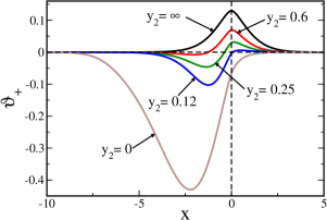
Figure 2: (color online) The scaling function $\vartheta_{+}(x,y_{1},y_{2})$ of the critical Casimir force (7) for the isotropic lattice with $K_{1}=K_{2}$ $y_{1}=h_{1}^{2}N=0$ and for the several values of $y_{2}=h_{2}^{2}N$.

The case with $h_{1}h_{2}<0$ can be approached from that with $h_{1}h_{2}>0$ by reversing the end spins between $x=1$ and $x=s+1$ on one face of the cylinder thereby creating an interface with terminations in the same face. This is followed by taking the limit as $M\to\infty$, as before. With $h_{j}>0,j=1,2$, we find the ratio of partition functions for strips with and without the interface to be:

$$e^{-sf^{\times}}=\int_{-\pi}^{\pi}\frac{d\omega}{2\pi}\frac{ie^{is\omega}\tan(\delta^{*}/2)\left(B^{+}-B^{-}A_{2}e^{-2N\gamma(\omega)}\right)}{1+A_{1}A_{2}e^{-2N\gamma(\omega)}}$$ (8)

where $B^{\pm}=\left(e^{\pm\gamma(\omega)}-e^{-4K_{2}}w_{1}\right)/(e^{\gamma(\omega)}-w_{1})$. We are interested in the limit $s\to\infty$ of the rhs of (8) per unit length. The asymptotics for large $s$ is dominated by the nearest singularity to the real axis in the strip $-\pi<\omega\leq\pi$. The branch cuts associated with $\sinh\gamma(\omega)$ do not occur and poles are simple zeros of the denominator of (8). Fortunately, the problem can be related to the diagonalisation problem of the transfer matrix in the direction $(1,0)$ AM (here we are transferring in $(0,1)$ direction) by looking for the solution in the variable $k$ such that $\omega=i{\hat{\gamma}}(k)$ and $\lim_{\epsilon\to 0^{+}}\gamma(i{\hat{\gamma}(k)\pm\epsilon})=\pm ik$, where the function ${\hat{\gamma}}(k)$ is defined as the Onsager function, but with $K_{1}$ and $K_{2}$ interchanged. Then finding zeros of the denominator of (8) becames equivalent to solving the spectrum discretisation condition for the strip transfer matrix in the $(1,0)$ direction, which was studied in detail in Ref. AM :

$$e^{2i(N+1)k}=e^{2i{\hat{\delta}}^{\prime}(k)}\frac{e^{ik}w_{1}-1}{e^{ik}-w_{1}}\frac{e^{ik}w_{2}-1}{e^{ik}-w_{2}}.$$ (9)

$e^{i{\hat{\delta}}^{\prime}(k)}$ is obtained from $e^{i\delta^{\prime}(k)}$ by interchanging $K_{1}$ and $K_{2}$. In the scaling limit $N\to\infty$, $K_{2}-K_{1}^{*}\to 0$ and $N(K_{2}-K_{1}^{*})=x$, we find $f^{\times}=(1/N)\lambda(x,u_{0})$. Hence the solution for the Casimir scaling function $\vartheta_{-}(\underline{r})=\vartheta^{\times}(\underline{r})+\vartheta_{+}(\underline{r})$ has the implicit form with

$$\vartheta^{\times}(\underline{r})=\frac{u_{0}^{2}-u_{0}{\underline{r}}\cdot\underline{\nabla}u_{0}}{N^{2}\lambda(x,u_{0})},$$ (10)

where $u_{0}({\underline{r}})$ solves the quantisation condition (9) in the scaling limit

$$e^{2iu}=-\frac{Z^{+}(0)}{Z^{-}(0)}\frac{Z_{1}^{-}Z_{2}^{-}}{Z_{1}^{+}Z_{2}^{+}},$$ (11)

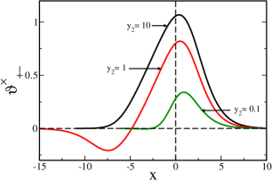
Figure 4: (color online) The excess scaling function $\vartheta^{\times}(x,y_{1},y_{2})$ of the critical Casimir force (10) for the isotropic lattice with $K_{1}=K_{2}$ $y_{1}=h_{1}^{2}N=1$ and for the several values of $y_{2}=h_{2}^{2}N$.

where $Z^{\pm}_{j}=Z^{\pm}(y_{j}),j=1,2$ is derived from $X_{\pm}(y)$ by replacing $\lambda(x,u)$ by $iu$. The derivatives of $u_{0}$ can be calculated straightforwardly from (11). In Figs. 3 and 4 we plot $\vartheta^{\times}$ as a function of $x$ evaluated numerically for some choices of the scaling variables $y_{1}$ and $y_{2}$. Our results for the special case of $y_{1}=y_{2}$ agree with those reported in Ref. napiorkowski ; the change of sign of the scaling function $\vartheta^{\times}$ is associated with the localisation-delocalisation transition parryevans . This feature remains for a slightly broken symmetry, i.e., for $y_{1}\approx y_{2}$ and $y_{1,2}$ small. For strongly asymmetric strips the excess scaling function of the critical Casimir force is always positive.

We now interpret (6) in terms of statistical mechanical ideas. Expanding the integrand gives

$$f^{\times}=\sum_{n=1}^{\infty}\frac{(-1)^{n}}{n}\int_{-\pi}^{\pi}\frac{d\omega}{4\pi}e^{-2Nn\gamma(\omega)}\left(C_{1}C_{2}\right)^{n}.$$ (12)

where $C_{j}(\omega)=\frac{A_{j}^{-}}{A_{j}^{+}}\tan\frac{\delta^{*}(\omega)}{2},j=1,2$. Although this is not immediately apparent, this is in fact a linked cluster expansion as we now show. Equation (12) can be understood by going back to the partition function formula in terms of a transfer matrix $V$

$$Z=\langle b_{1}\mid V^{N}\mid b_{2}\rangle$$ (13)

where $\mid b_{j}\rangle$ describes the edge state with field $h_{j},j=1,2$. Instead of using the Schultz, Mattis and Lieb technology, this can be developed by expanding with basis of eigenvectors of $V$ giving

$$\frac{Z}{\Lambda_{max}^{N}}=\sum_{n=0}^{\infty}\sum_{(\omega)_{2n}}\frac{e^{-N\sum_{j=1}^{2n}\gamma(\omega_{j})}}{(2n)!}\langle b_{1}\mid(\omega)_{2n}\rangle\langle(\omega)_{2n}\mid b_{2}\rangle,$$ (14)

where $\mid(\omega)_{2n}\rangle$ denotes a $2n$-fermion eigenstate of $V$ LMS . This would certainly not be the chosen way of obtaining (6), since we would need to evaluate the matrix elements $\langle b_{1}\mid(\omega)_{2n}\rangle,\langle(\omega)_{2n}\mid b_{2}\rangle$; this has been done with some effort and the result is typically Wick-theoretic in form:

$$\langle b_{j}\mid(\omega)_{2n}\rangle=\sum_{m=2}^{2n}(-1)^{m}f_{j}(\omega_{1},\omega_{m})\langle b_{j}\mid\Delta_{1m}(\omega)_{2n}\rangle$$ (15)

where $\Delta_{1m}(\omega)_{2n}=(\omega_{2},\ldots\omega_{m-1},\omega_{m+1}\ldots\omega_{2n})$ and $f_{j}(\omega_{1},\omega_{2})=iC_{j}(\omega)\delta_{\omega_{1},-\omega_{2}}$ is the contraction function or, alternatively, a scattering matrix element for a pair of fermions off the wall described by $\mid b_{j}\rangle$. Notice that since the $A^{\pm}_{j}(\omega)$ are even, but $\tan\frac{1}{2}\delta^{*}(\omega)$ is odd, the contraction is antisymmetric as it should be for fermions. Thus, (15) is a Pfaffian Pf . The graphical representation of (14) and (15) is discussed in DBA78 . For each $n$ we have a weighted sum of disjoint loops, each having an even number of vertices, the vertex weight $C_{j}(\omega)$ and the Kronecker delta edge weight. The occurrence of the Kronecker delta in the contraction function is mandated by translational symmetry. Thus, the multiple sum for each loop becomes just a single sum on implementing the deltas. Asymptotically as $M\to\infty$, each such sum is to leading order $M$ times a single integral. We can now apply the linked cluster theorem to exponentiate (14). Eq. (12) is recaptured, for the excess free energy per unit length in the $(1,0)$ direction since the factor of $1/n$ in (12) comes directly from a symmetry number argument uhlenbeck . Each term is then to be thought of as a weight of a ”loop” with $2n$ vertices. The loop is reflected $n$ times off the upper boundary and $n$ times off the lower boundary, with ”momentum” conservation at each reflection; thus $n$ maybe thought of as a topological quantum number. Starting from (13), (14) and (15), we have re-derived (12), in a way which allows us to identify the multiplier of $\exp 2N\gamma(\omega)$ in (6) as a product of two scattering matrix elements, one from each edge. Clearly $\gamma(\omega)$ in (14) is a Fermion energy. Thus we have a complete intuitive understanding of (6). We can take the scaling limit either in (12) or (6) (as we have already done) with the same outcome. This procedure even converges after taking $T\to T_{c}$ in either (12) or (6), since then $\gamma(\omega)\propto\mid\omega\mid$.

Two approximation schemes are in order. Firstly, we could consider how well partial sums of the virial series (12) approximate the exact result, so that we can assess the contribution of the different reflection number sectors to the result. Secondly, in the scaling limit the one-particle energy should be universal. The same is not likely to be true for the scattering matrix elements. Correlation droplet theory DBA83 provides an approximate method for calculating them and thus for extending the scope of our results.

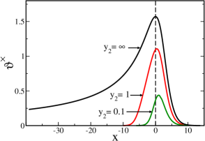
Figure 3: (color online) The excess scaling function $\vartheta^{\times}(x,y_{1},y_{2})$ of the critical Casimir force (10) for the isotropic lattice with $K_{1}=K_{2}$ $y_{1}=h_{1}^{2}N=\infty$ and for the several values of $y_{2}=h_{2}^{2}N$.

In this Letter, we have described new, general, exact results for the critical Casimir force in a planar, rectangular Ising ferromagnet with applied fields $h_{1}$ and $h_{2}$ on the edges. Each field can have arbitrary sign and magnitude. Both with $h_{1}h_{2}>0$ and with $h_{1}h_{2}<0$, we show that the force can be attractive or repulsive, according to the tuning of the parameters. The compensation of attractive, quantum van der Waals forces which this will allow has implications which may well prove crucial for applications. Mean field calculations are in qualitative agreement with our results mohry . There are also related results from the continuum model  diehl . We also interpret the representation of the Casimir force as in (5), (6) and (12) in terms of the linked cluster expansion. This suggest an associated droplet picture which enhances the original finite size scaling ideas of Privman and Fisher privman in this context; this will also give new, systematic approximations for calculating critical Casimir forces in planar systems and perhaps even in $d=3$. Our results can be directly applied to e.g. $2d$ binary fluid membranes with protein inclusions close to the demixing point membranes .

DBA acknowledges Max-Planck-Gesellschaft for hospitality.

References

- (1) H. B. Casimir, Proc. K. Ned. Akad. Wet. 51, 793 (1948).
- (2) M. E. Fisher and P. G. de Gennes, C. R. Acad. Sci. Paris Ser. B 287, 207 (1978) .
- (3) M. Krech, Casimir Effect in Critical Systems (World Scientific, Singapore, 1994); J. Phys.: Condens. Matter 11, R391 (1999).
- (4) G. Brankov, N. S. Tonchev, and D. M. Danchev, Theory of Critical Phenomena in Finite-Size Systems (World Scientific, Singapore, 2000).
- (5) V. Privman and M. E. Fisher, J. Stat. Phys. 33, 385 (1983).
- (6) R. Evans and J. Stecki, Phys. Rev. B 49 (1994) 8842.
- (7) D. B. Abraham, Studies in Appl. Math. 50, 71 (1971).
- (8) L. Onsager, Phys. Rev. 65, 117 (1944).
- (9) T. D. Schultz, D. C. Mattis, and E. H. Lieb, Rev. Mod. Phys. 36, 856 (1964).
- (10) D. B. Abraham, Phys. Rev. Lett. 44, 1165 (1980).
- (11) A. Maciołek and J. Stecki, Phys. Rev. B 54, 1128 (1996).
- (12) P. Nowakowski and M. Napiórkowski, Phys. Rev. E 78, 060602(R) (2008); e-preprint arXiv:0908.1775v1.
- (13) A. O. Parry and R. Evans, Phys. Rev. Lett. 64, 439 (1990); Physica A 181, 250 (1992).
- (14) E. R. Caianiello, Combinatorics and renormalization in quantum field theory, (Benjamin, Reading, Mass., 1973).
- (15) D. B. Abraham, Commun. Math. Phys. 50, 181 (1978).
- (16) G. E. Uhlenbeck and G. W. Ford, Lectures in Statistical Mechanics, (American Mathematical Society, Providence, RI, 1963).
- (17) D. B. Abraham, Phys. Rev. Lett. 50, 291 (1983).
- (18) T. F. Mohry, A. Maciołek, and S. Dietrich, preprint (2009).
- (19) F. M. Schmidt and H. W. Diehl, Phys. Rev. Lett. 101, 100601 (2008).
- (20) A. R. Honerkamp-Smith et al, Biophys. J. 95, 236 (2008).