Changing growth conditions during surface growth

Abstract

Motivated by a series of experiments that revealed a temperature dependence of the dynamic scaling regime of growing surfaces, we investigate theoretically how a nonequilibrium growth process reacts to a sudden change of system parameters. We discuss quenches between correlated regimes through exact expressions derived from the stochastic Edwards-Wilkinson equation with a variable diffusion constant. Our study reveals that a sudden change of the diffusion constant leads to remarkable changes in the surface roughness. Different dynamic regimes, characterized by a power-law or by an exponential relaxation, are identified, and a dynamic phase diagram is constructed. We conclude that growth processes provide one of the rare instances where quenches between correlated regimes yield a power-law relaxation.

I Introduction

Because of their ubiquity in nature, nonequilibrium growth processes have been the subject of numerous studies during the last two decades Mea93 ; Hal95 ; Bar95 . Remarkably, these studies revealed very general properties of growing interfaces that are encountered in a large variety of growth processes, ranging from crystal growth to tumor growth. In this context, due to its obvious technological relevance, thin film growth has been one of the major research thrusts.

From the theoretical point of view, many important insights into the universal aspects of nonequilibrium growth processes have been obtained through the study of stochastic differential equations and of simple model systems Kru97 ; Kru95 . One of the simplest approach is due to Edwards and Wilkinson 1982SE who described the surface growth due to particle sedimentation by $\partial h({\bf x},t)/\partial t=\nu\nabla^{2}h({\bf x},t)+u$, where $h({\bf x},t)$ is the surface height at time $t$ at a site ${\bf x}$ of a $d$-dimensional substrate (of area ${\cal A}$) and $u$ represents a constant flux of deposition. The physical origin of the “diffusion constant” $\nu$ can be traced to the surface tension as well as $T$, the temperature of the substrate. When noise is added to this and the process is viewed from a co-moving frame of the steady state (i.e., $h({\bf x},t)-ut\rightarrow h({\bf x},t)$), we arrive at the stochastic Edwards-Wilkinson (EW) equation

$$\frac{\partial h({\bf x},t)}{\partial t}=\nu\nabla^{2}h({\bf x},t)+\eta({\bf x},t)$$ (1)

where $\eta({\bf x},t)$ is a Gaussian white noise with zero mean and covariance $\left\langle\eta({\bf x},t)\eta({\bf y},s)\right\rangle=D\delta^{d}({\bf x}-{\bf y})\delta(t-s)$. A microscopic realization of the Edwards-Wilkinson equation was soon proposed by Family 1986FF ; Bar95 (see also Ref. [Rot06, ] for a recent more in-depth comparison of that model with the EW equation). In the random deposition with surface relaxation (RDSR) process particles drop from randomly chosen sites over the surface. Instead of sticking to the surface at the point of impact, the particles are allowed to explore the nearest vicinity of that point and are finally incorporated into the surface at the neighboring site with lowest height. This diffusion step smoothes the surface and yields correlated growth.

The roughness of a growing surface is characterized by the time dependent mean interface width

$$W(t)=\sqrt{\langle\left(h-\overline{h}\right)^{2}\rangle}$$ (2)

where $\overline{h}(t)\equiv\int h({\bf x},t)d^{d}{\bf x}/{\cal A}$ is the mean surface height at time $t$. In many instances the mean interface width (after an initial regime of random surface growth when starting from a flat initial condition) displays a power-law dependence on time, $W(t)\sim t^{\beta}$, before saturating at a value $W\sim L^{\alpha}$ where $L$ is the size of the system. The growth exponent $\beta$ and the roughness exponent $\alpha$ are universal quantities that characterize large classes of growth systems belonging to the same growth universality class. Thus for the Edwards-Wilkinson universality class one finds for a one-dimensional substrate $\beta=1/4$ and $\alpha=1/2$. Other universality classes have also been found Kru97 ; Kru95 , some of which, as for example the Kardar-Parisi-Zhang (KPZ) Kar86 and the conserved KPZ universality classes Wol90 ; Sar91 , are of direct relevance for thin film growth.

The morphology of growing structures can depend crucially on experimental parameters as for example the flux of deposited particles or the substrate temperature Jen99 . Different experimental groups have reported a temperature dependence of the roughness of growing or sputtered surfaces, and temperature dependent values of the growth exponents have been found in some systems Ern94 ; Yan94a ; Yan94b ; Ell96 ; Smi97a ; Smi97b ; Sto00 ; Kal01 ; Bot01 ; Els04 ; Fer06 . Systems for which this has been observed include homoepitaxial growth on Cu(001) Ern94 ; Bot01 , Ag(100) Ell96 ; Sto00 , and Ag(111) Ell96 , amorphous thin-film growth Els04 , growth of CdTe polycrystalline films Fer06 , molecular-beam epitaxy growth of Si/Si(111) Yan94b , as well as ion-sputtered Si(111) Yan94a , Ge(001) Smi97a ; Smi97b or Pt(111) Kal01 surfaces. The dependence of the roughness on temperature can be rather involved, yielding different types of behavior for different systems, depending on how diffusion takes place and whether additional smoothening mechanisms are present. In many instances one observes that growth becomes increasingly rougher with decreasing temperature, yielding an increase of the value of $\beta$. On the other hand, some experiments Els04 ; Fer06 revealed an increase of the global roughness with temperature.

The observation of a transition between different dynamic scaling regimes due to a change of experimental conditions is very intriguing and raises the question how a growing surface evolves from one regime to another after a sudden change of, for example, the substrate temperature. We are not aware of any experimental study of growth processes where this kind of protocol has been implemented. However, we expect that the intriguing results reported here will motivate future experimental studies along similar lines. In this paper we discuss exact results derived from the EW equation with a variable diffusion constant, which allows us to investigate systematically the changes in the surface roughness in case growth conditions are changed during the growth process. Interestingly, different dynamic regimes are encountered, some of which are characterized by a power-law relaxation. Here, we do not have a specific experimental system in mind. Instead, our interest is broader, namely, to understand universal responses of a growing surface to sudden changes of experimental parameters through the study of simple models.

It is to be noted that our study is complementary to an earlier investigation due to Majaniemi, Ala-Nissila, and Krug Maj96 . Similarly to our work, these authors studied the impact of a change of growth conditions on processes described by linear growth equations. Whereas we discuss in the following the effects of a variable diffusion constant, Majaniemi et al. analyzed how the growing surface reacts to a change of the noise in the system.

There is also a second, theoretical motivation for our study. Sudden changes of external conditions, as for example due to a temperature quench, have been investigated in recent years in a large variety of systems, ranging from magnetic systems to glasses Cug ; Ple08 ; Hen09 . In the most common setting, a system initially prepared in some equilibrium state is suddenly brought out of equilibrium through a temperature quench. If the system is characterized by slow, non-exponential relaxation (as it is the case for a ferromagnet quenched to or below the critical point), interesting nonequilibrium processes and aging phenomena are observed Hen09 . Some studies also focused on slow relaxation encountered in up-quenches in which a magnetic system initially in the ground state is quenched to the critical point Gar05 ; Pau07 . Interestingly, however, slow relaxation is usually not observed when both the initial and final temperatures are below the critical point. Indeed, for models with a discrete global symmetry such as Ising or Potts models a competing ordered state can not be reached if the starting point is close to one of the minima of the equilibrium free energy. Consequently, non-exponential relaxation is only encountered in this type of quench if the system has a continuous symmetry, as it is for example the case of the $XY$ model Ber01 ; Pic04 . As we will show in this paper, surface growth processes constitute an interesting class of systems where a change of parameters yields a transition from one correlated state to another characterized by a power-law relaxation.

The paper is organized in the following way. In Section II we discuss the dependence of the surface width, derived from the EW equation, on the value of the diffusion constant. Section III is devoted to the study of the time evolution of the surface roughness following a sudden change of the diffusion constant. We thereby identify different dynamic regimes and present a dynamic phase diagram that summarizes the possible responses of the growing interface. Finally, we end with a summary and outlook in Section IV.

II Interface width

In order to study the effect of a change of external conditions on simple growth processes we consider the Edwards-Wilkinson equation (1) with a variable diffusion constant $\nu$ (a microscopic realization of this process has recently been discussed in Cho09 ). When describing a deposition or growth process by this equation, one implicitly assumes that $\nu$ and the noise amplitude $D$ depend on the experimental parameters, as for example the temperature $T$. In the following we will not need to know the explicit dependence of $\nu$ and $D$ on these parameters (which would be system dependent), and study how the interface width changes when changing the value of $\nu$. The reaction of the growing surface to a change of the noise has been studied in Maj96 .

The stochastic EW equation (1), can be solved exactly to give us for a fixed value of $\nu$ the width (squared)

$$W^{2}\left(t\right)=\frac{D}{2\nu L}\sum_{n}\frac{1-e^{-2\nu tk_{n}^{2}}}{k_{n}^{2}}$$ (3)

where $k_{n}=2\pi n/L$ and the sum is over $\left[-L/2,L/2\right]$ but excluding the zero mode: $n=0$. In Figure 1a,c we show the time dependence of the surface width for, respectively, the case with fixed $L=1000$ at different $\nu$’s and the case with a fixed $\nu=0.1768$ and various $L$’s. As for the RDSR process one distinguishes three regimes separated by two crossover points: a random deposition (RD) regime, followed by a EW regime, with a final crossover to the saturation regime. In contrast to Family’s original model, the initial RD process is not confined to very early times $t\leq 1$ but might extend to larger times. In fact, the crossover time $t_{1}$ between the RD and the EW regimes is shifted to higher values for decreasing diffusion constants and diverges in the limit of vanishing $\nu$. As the crossover is smeared out, we identify the crossover point with the intersection point of the straight lines fitted to the two linear regimes in the log-log plots. We have the identity $W^{2}=t$ in the RD regime, yielding the width $W_{1}=\sqrt{t_{1}}$ at the crossover point. In the EW regime the relation between width and deposition time changes to $W\propto t^{1/4}$. This regime extends up to a second crossover point $(t_{2},W_{2})$, whose precise location depends on the values of $\nu$ and $D$ and beyond which the final saturation regime prevails. The crossover between the different regimes is further illustrated in Fig. 1b,d where we show the time evolution of the effective exponent

$$\beta_{eff}=\frac{d\log W}{d\log t}=\frac{\nu t\sum\limits_{n}e^{-2\nu tk_{n}^{2}}}{\sum\limits_{n}\left[1-e^{-2\nu tk_{n}^{2}}\right]/k_{n}^{2}}~{}.$$ (4)

for the two cases.

 

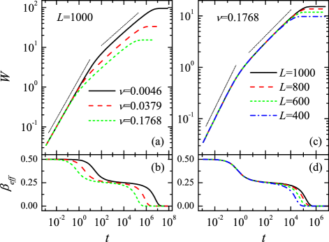
Figure 1: (a) Log-log plot of the surface width vs time for a system of size $L=1000$ and different diffusion constants. The dotted lines have the slopes $1/2$ and $1/4$ expected in the random deposition and EW regimes, respectively. The locations of both crossover points depend on the diffusion constant. The data are obtained from the exact solution of the EW stochastic equation. (b) Time evolution of the effective exponent (4) for the data shown in (a). (c) Log-log plot of the surface width vs time for systems of different sizes evolving at the same diffusion constant $\nu=0.1768$. (d) Time evolution of the effective exponent (4) for the data shown in (c). The data in this and the following figures have been obtained for $D=1$.

We end this Section with a few remarks:

• The (“first”) crossover from the RD to the EW regime, denoted by $\left(t_{1},W_{1}\right)$, depends only on $\nu$. For the range of $L$’s we explored, we find $W_{1}^{2}=t_{1}\cong\tau/\nu$, with a constant $\tau\cong 0.148$. In the $L\rightarrow\infty$ limit, $\tau\rightarrow 1/2\pi$ (as shown in the Appendix, see also Ama92 ).

• The (“second”) crossover from the EW to the saturation regimes, denoted by $\left(t_{2},W_{2}\right)$, depends on both $\nu$ and $L$. $W_{2}$ may be identified with the saturation width, i.e., $\left(DL/8\pi^{2}\nu\right)\sum_{n}n^{-2}$ Ama92 . Combining this result with the line drawn through the EW regime, we arrive at $t_{2}=\left(L/24\tau\right)^{2}t_{1}$ (see Appendix).

III Sudden change of growth conditions

With a clear picture of the properties of a surface growing under a constant diffusion constant, we proceed to study the time evolution of the roughness when $\nu$ is suddenly changed. To investigate the response of the growth process to this change, we use the following protocol: We start at $t=0$ with a flat surface and let the surface grow at $\nu_{i}$ until time $t=s$, at which point we change the diffusion constant to the final value $\nu_{f}$. The change of roughness is then monitored through the time evolution of $W^{2}$.

As our system displays three different roughness regimes (RD, EW, and saturation), there can be in principle nine scenarios for the change to be arranged. They can be distinguished conveniently by (1) $\nu_{i}$, the diffusion constant of the initial growth, (2) $\nu_{f}$, the final value of the diffusion constant, and (3) $s$, the time at which $\nu$ is suddenly changed. By choosing these three controls judiciously, we can access all the scenarios. However, covering all cases in detail is not the aim of this paper. Instead, we are interested in the new phenomena associated with the $t$-dependence of the width, $W^{2}(t,s)$, after (up- or down-) quenches. Obviously, for $t\gg s$, the surface roughness will settle into the value in an “unperturbed” system, grown at $\nu_{f}$ from the start. Denoted by $W_{u}^{2}(t)$, it is just expression (1) with $\nu=\nu_{f}$. We also refer to this as the “reference system.” To highlight the changes, we also study the difference (with $t>s$)

$$\Delta W^{2}(t,s)=|W^{2}(t,s)-W_{u}^{2}(t)|$$ (5)

between quenched system and the reference. Clearly, this quantity reveals how the roughness of the growing surface adapts itself to the new “experimental” condition, and behaves very differently for the various cases. Our goal is to map out the regions in the $\nu_{i}$-$\nu_{f}$-$s$ space corresponding to the novel behavior following a quench.

To be precise, we will evolve the height $h(x,t)$ starting from $h(x,0)=0$ with $\nu_{i}$ to time $s$ and then continue with $\nu_{f}$ until time $t$. At that point, we compute the width squared and denote it by $W^{2}(t,\nu_{f};s,\nu_{i})$.

Our starting point is the exact solution of (1)

$$\tilde{h}(k_{n},t) = e^{-\nu_{f}k_{n}^{2}(t-s)}\,\int\limits_{0}^{s}\,dt^{\prime}\,e^{-\nu_{i}k_{n}^{2}(s-t^{\prime})}\tilde{\eta}(k_{n},t^{\prime})$$ (6)

$$+\int\limits_{s}^{t}dt^{\prime\prime}\,e^{-\nu_{f}k_{n}^{2}(t-t^{\prime\prime})}\tilde{\eta}(k_{n},t^{\prime\prime})$$

written here in terms of the Fourier amplitudes for $h(x,t)$ and $\eta(x,t)$: $\tilde{h}(k_{n},t)=\int\,dx\,e^{ik_{n}x}\,h(x,t)$, etc. Since the noise is delta-correlated, $\langle|\tilde{h}|^{2}\rangle$ simplifies so that the width square is

$$W^{2}(t,\nu_{f};s,\nu_{i}) = \frac{D}{L}\sum\limits_{n}\left[e^{-2\nu_{f}k_{n}^{2}(t-s)}\int\limits_{0}^{s}\,dt^{\prime}\,e^{-2\nu_{i}k_{n}^{2}(s-t^{\prime})}\right.$$ (7)

$$\left.+\int\limits_{s}^{t}dt^{\prime}\,e^{-2\nu_{f}k_{n}^{2}(t-t^{\prime})}\right]~{}.$$

Since the width square $W_{u}^{2}(t,\nu_{f})$ of the unperturbed system is given by

$$W^{2}(t,\nu_{f};s,\nu_{i})=\frac{D}{L}\sum\limits_{n}\int\limits_{0}^{t}dt^{\prime}\,e^{-2\nu_{f}k_{n}^{2}(t-t^{\prime})}~{},$$ (8)

we arrive at the exact result for the difference $\Delta W^{2}=\left|W^{2}(t,\nu_{f};s,\nu_{i})-W_{u}^{2}(t,\nu_{f})\right|:$

$$\Delta W^{2} = \left|\frac{D}{L}\sum\limits_{n}e^{-2\nu_{f}k_{n}^{2}(t-s)}\right.$$ (9)

$$~{}~{}~{}~{}\left.\int\limits_{0}^{s}\,dt^{\prime}\,\left[e^{-2\nu_{i}k_{n}^{2}(s-t^{\prime})}-e^{-2\nu_{f}k_{n}^{2}(s-t^{\prime})}\right]\right|$$

$$= \left|\frac{D}{L}\sum\limits_{n}e^{-2\nu_{f}k_{n}^{2}(t-s)}\right.$$

$$~{}~{}~{}~{}\left.\left[\frac{1-e^{-2\nu_{i}k_{n}^{2}s}}{2\nu_{i}k_{n}^{2}}-\frac{1-e^{-2\nu_{f}k_{n}^{2}s}}{2\nu_{f}k_{n}^{2}}\right]\right|~{}.$$

For later convenience, we define $\Omega\equiv\nu_{f}\Delta W^{2}(t,\nu_{f};s,\nu_{i})$ and note that it depends only on three scaling variables:

$$\mu\equiv\nu_{i}/\nu_{f},\quad\sigma\equiv\nu_{f}s,\quad\rho\equiv t/s\,\,.$$

Explicitly, we have

$$\Omega(\mu,\sigma,\rho) \equiv \nu_{f}\Delta W^{2}$$ (11)

$$= \left|\frac{D}{L}\sum\limits_{n}e^{-2k_{n}^{2}\sigma\left(\rho-1\right)}\right.$$

$$~{}~{}~{}~{}\left.\left[\frac{1-e^{-2k_{n}^{2}\mu\sigma}}{2k_{n}^{2}\mu}-\frac{1-e^{-2k_{n}^{2}\sigma}}{2k_{n}^{2}}\right]\right|\,\,.$$

To set the stage for discussions, we begin with the data for some typical cases, all with $s=10^{5}$, shown in Fig. 2. In order to be able to discuss the different cases for a fixed $s$, we must work with a relatively small system: $L=400$. The dashed lines in (a-c) represent $W_{u}^{2}(t)$ in an unperturbed system. With $\nu_{f}=4.7\cdot 10^{-10}$, $0.00047$, and $0.18$, the surface is, at the time of the quench, in the (a) RD, (b) EW, and (c) saturation regimes, respectively. The corresponding differences, $\Delta W^{2}(t,s)$, are shown in Fig. 2d-f.

The effects of two up-quenches into the RD regime, from the EW ($\nu_{i}=0.0046$) and the saturation ($\nu_{i}=0.23$) regimes, are displayed in Fig. 2a. As Fig. 2d shows, for quenches into RD, the width $W^{2}(t,s)$ cannot reach that of the reference system, $W_{u}^{2}(t)$. The “best” $\Delta W^{2}(t,s)$ can achieve is a constant. The physical origin of this behavior lies in the linear growth of $W^{2}$ in the RD regime. Thus, for two unperturbed systems started at different times (say, $t=t_{0}$ and $t_{1}$), the difference $W_{0}^{2}-W_{1}^{2}$ is just a constant: $t_{1}-t_{0}$. In our case, the correlated growth up to time $s$ endowed our surface with a smaller $W^{2}\left(s\right)$ than the reference $W_{u}^{2}(s)$. Immediately after the quench, correlated growth is simply replaced by independent growth of different columns and the width $W^{2}\left(s\right)$ is “frozen” in as a kind of “initial condition” (at $t=s$). As a result, the difference $\Delta W^{2}=W_{u}^{2}(t)-W^{2}(t,s)$ remains at the value $W_{u}^{2}(s)-W^{2}\left(s\right)$. Of course, if we follow these two systems further in time, $\Delta W^{2}$ will eventually vanish.

Turning next to quenches to the EW regime, we found the most interesting behavior (Fig. 2b,e). The difference $\Delta W^{2}$ initially decreases rapidly, before crossing over to a slower, power-law decay at larger times ($t\gg s$):

$$\Delta W^{2}\sim t^{-\gamma}$$ (12)

For example, for the cases shown in Fig. 2e, we measure close to the end of the time interval the exponents $\gamma=0.72$ for $\nu_{i}=0.23$, $\gamma=1.24$ for $\nu_{i}=0.0046$, and $\gamma=1.65$ for $\nu_{i}=4.7\cdot 10^{-10}$. As we argue below, these are effective values, the asymptotic values of $\gamma$ being $1/2$ or $3/2$. Below we will also discuss in more detail the conditions under which these values can be expected. Finally, for a quench to the saturation regime, $\Delta W^{2}$ decays exponentially:

$$\Delta W^{2}\sim\exp(-\kappa t)$$ (13)

with a decay constant $\kappa$ that depends both on the value of the final diffusion constante $\nu_{f}$ and on the system size $L$.

 

Figure 2: (Color online) (a-c) Time evolution of the width square in case the diffusion constant is changed after $10^{5}$ time steps. The dashed lines show $W_{u}^{2}(t)$ for an unperturbed surface growing at constant $\nu_{f}$. In (a) the quench is to the RD regime, whereas in (b) and (c) the quenches are to the EW and saturation regimes, respectively. (d-f) The same cases as shown in (a-c), but now the difference $\Delta W^{2}$, see Eq. (5), is plotted. Qualitative different behavior is observed, depending on the regime that the unperturbed system has at the quench time.

Up to now, we have shown only the simplest situation where the system is well within a given initial regime at the moment of the quench and, in addition, that it has time to relax into a well defined regime of the reference system. Clearly, as we let the final system evolve further, it may crossover to a different regime (e.g., in case of Fig. 2a,d a crossing over to the EW and saturation regimes will take place for larger $t$). Therefore, we should expect the general relaxation process to be quite complex.

The closed forms (9,11) are not particularly transparent, as they involve all possible crossover behaviors. To shed some light on the various scenarios, we consider some limiting cases where simple properties (exponentials and powers) can be extracted. A straightforward case is $\nu_{f}(t-s)\gg L^{2}$, so that $\nu_{f}k_{n}^{2}(t-s)$ is always large. Then, the leading decay is exponential, namely $e^{-8\pi^{2}\nu_{f}(t-s)/L^{2}}$, since the other terms in the sum will be much smaller:

$$\left(e^{-8\pi^{2}\nu_{f}(t-s)/L^{2}}\right)^{4},~{}\left(e^{-8\pi^{2}\nu_{f}(t-s)/L^{2}}\right)^{9},\cdots$$

$$~{}~{}~{}~{}\ll e^{-8\pi^{2}\nu_{f}(t-s)/L^{2}}~{}.$$ (14)

In the opposite limit, where $\nu_{f}s,\nu_{i}s\ll 1$, we have

$$\left[\frac{1-e^{-2\nu_{i}k_{n}^{2}s}}{2\nu_{i}k_{n}^{2}}-\frac{1-e^{-2\nu_{f}k_{n}^{2}s}}{2\nu_{f}k_{n}^{2}}\right]\cong(\nu_{f}-\nu_{i})s^{2}k_{n}^{2}$$ (15)

to leading order. The summation over $n$ then yields, for $t-s\gg 1$, a power-law decay: $t^{-3/2}$, i.e., $\gamma=3/2$.

In order to explore the three-dimensional parameter space $\left(\mu,\sigma,\rho\right)$ in a comprehensive way, we evaluate numerically the closed form (11). The exponent $\gamma$ can be defined effectively as $-d\log(\Omega)/d\log(t)$. In Fig. 5 we show the contour plot of $\gamma$ as a function of $\mu$ and $\sigma$ for $\rho=64$. This plot reveals four different regimes: the regime where $\Omega$ or $\Delta W^{2}$ is constant (labeled by $\gamma=0$), two power-law regimes with values $\gamma=1/2$ and $\gamma=3/2$, and finally a regime of exponential decay for large $\sigma$. The different regimes are separated by crossover regions where the effective exponent does not lock-in into one of the values 0, 1/2, or 3/2.

 

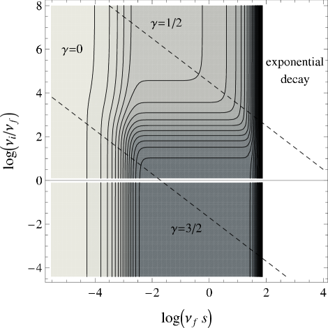
Figure 3: Contour plot of $\gamma$ as a function of $\nu_{f}s$ and $\nu_{i}/\nu_{f}$ for $t/s=\rho=64$. Four different regimes, separated by crossover regions, are identified. The two dashed lines separate the three qualitatively different types of behavior encountered when plotting the effective exponent as a function of $t$, see Fig. 5.

Fig. 4a shows how the extensions of the four regimes depend on the value of $\rho$ in cases where $\rho\gg 1$. Interestingly, an increase of the value of $\rho$ mainly shifts the contours in the $\log(\sigma)$ vs. $\log(\mu)$ plot along the $(-1,1)$ direction. This is shown in Fig. 4b where we plot $\log(\nu_{f}t)=\log(\sigma\rho)$ vs. $\log(\nu_{i}s/\nu_{f}t)=\log(\mu/\rho)$. This way of plotting indeed leads to an approximate data collapse, which gets better for larger values of $\rho$. That this data collapse is only approximate also follows from inspection of the exact solution (11). Still, Fig. 4b nicely allows us to visualize the extent of the different dynamic regimes for large ratios $\rho$.

 

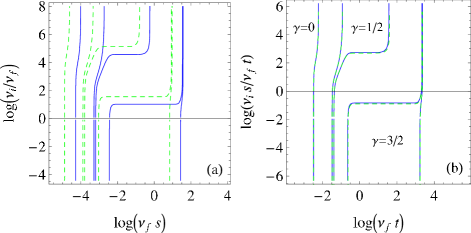
Figure 4: (Color online) (a) Contour plots of $\gamma$ as a function of $\nu_{f}s=\sigma$ and $\nu_{i}/\nu_{f}$ for $t/s=\rho=64$ (full lines) and $256$ (dashed lines). Only contours bounding the $\gamma=0$, $1/2$ and $3/2$ regimes are shown. (b) The same contour plots as shown in (a) but as a function of $\nu_{f}t$ and ${\nu_{i}s}/{\nu_{f}t}$. An approximate collapse of the contours is observed.

Finally, in Fig. 5, we discuss the change of the effective exponent $\gamma$ as a function of $t$ for various values of $\mu$ (and $s=10^{5}$). Note that an increasing time $t$ corresponds in Fig. 3 approximately to a cut along the $(-1,1)$ direction, so that we can distinguish three typical scenarios, separated by the dashed lines there. Along the upper dashed line, Fig. 5a shows the effective exponent rising to the $\gamma=1/2$ plateau where it remains for a long time before crossing over to the regime where the difference $\Delta W^{2}$ vanishes exponentially fast (“$\gamma=\infty$”). For the region above this line in Fig. 3, we can expect similar results. Along the lower dashed line, the same behavior is seen, except that the plateau value is now $\gamma=3/2$ (Fig. 5c). This can also be expected for the region below this lower dashed line in Fig. 3. Between these two protocols, a more complex behavior is encountered, as the effective exponent shows some tendency to lock-in at both values 1/2 and 3/2 (see Fig. 5b). We should remind the reader that the $\gamma\left(t\right)$ curves shown here are applicable for all varieties of quenches (different quench times, as well as different initial and final values of $\nu$) as long as the rescaled time $\nu_{f}s$ is fixed.

 

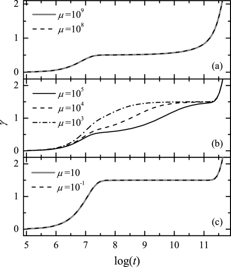
Figure 5: The three different quench types illustrated by the time dependence of the effective exponent $\gamma$. In all cases the quench takes place at $s=10^{5}$. Type (a) includes quenches with initial conditions $\nu_{f}s$ and $\nu_{i}/\nu_{f}$ located above the upper dashed line in Fig 4. For type (b) the starting point is located between the two dashed lines in Fig 4, wheres for type (c) the initial conditions put the starting point below the lower dashed line.

It is interesting to note that a change of the noise during the growth process also yields a power-law relaxation, as discussed in Maj96 . Thus for the one-dimensional EW equation it was observed that $\Delta W^{2}\sim t^{-1/2}$ if the system is in the EW regime before and after changing the noise of the system. The situation studied in Maj96 is therefore comparable to our case, even though we do observe a richer behavior when changing the diffusion constant.

IV Discussion and outlook

The morphology and roughness of growing surfaces depend in a crucial way on experimental conditions. Motivated by various observations of a change of the roughness universality class when changing experimental conditions, we have studied in this work how a growth process reacts to a sudden change of the diffusion constant. Exploiting the fact that the stochastic EW equation can be solved exactly, we carried out a comprehensive study of the response of the growing interface. Four main relaxation regimes, separated by crossovers, were identified. For extremely long times any finite system will eventually relax in an exponential way, due to the presence of the saturation regime, but this only takes place after an earlier power-law relaxation. For finite times, a growing surface rapidly reacts to a change of $\nu$ such that its morphology (roughness) approaches that of a reference system that was allowed to grow under stable external conditions. If the change of growth conditions takes place at a time where both the quenched and the reference system are in a correlated growth regime, than the relaxation process is governed by power-laws over many time decades. This is our main result (see also Maj96 ), and we expect this to hold true for other systems.

Of course, we do not expect that our results for a one-dimensional system can be applied quantitatively to any of the experimental systems in which a temperature dependence of the roughness exponent has been observed. Nevertheless, we expect that these results should be generic for growth processes with a sudden change of external conditions, and that the intriguing signatures revealed in our study can be generalized to more realistic models, so that they can be observed in experiments on physical systems.

From a more theoretical point of view, our study reveals that growth processes provide one of the rare cases where a power-law relaxation is generically observed when quenching from one correlated state to another. More specifically, the exactly solvable Edwards-Wilkinson equation allows us to derive analytical expressions, thus permitting a complete investigation of the various possible scenarios. It is to be expected that the power-law relaxation encountered at a quench also entails interesting aging processes not studied in the past. Indeed, in the few published studies of aging in growth processes Rot06 ; Bus07 ; Bus07a constant model parameters were always assumed.

Our study can be extended in various directions. On the one hand, we can study quenches in systems where the interface is stabilized not by surface tension, but by a curvature Hamiltonian. The simplest case is given by the noisy Mullins-Herring equation Mul63 ; Wol90 . As this is again a linear stochastic differential equation, we can follow the same strategy as in the present work and investigate the response to a temperature quench by analyzing exact expressions. On the other hand, we can also extend our study to systems that are of direct relevance for thin film growth: the Kardar-Parisi-Zhang (KPZ) Kar86 and the conserved KPZ universality classes Wol90 ; Sar91 . As exact expressions for these non-linear systems are not available, we plan to integrate these equations numerically and to simulate quenches in microscopic models belonging to the same universality classes.

Appendix

Here, we show how to compute the first crossover time $t_{1}$ in the limit of infinite $L$ (see also Ama92 ). Since this point is defined as the intersection of the RD regime ($W^{2}=Dt$) and the EW regime ($W^{2}\cong At^{1/2}$), we have

$$t_{1}=(A/D)^{2}$$ (16)

so that the problem reduces to finding the amplitude $A$ associated with EW growth. For $L\rightarrow\infty$ , the sum in expression (3) can be replaced by an integral, which can be computed to extract $A$. Further simplification occurs if we consider $\partial_{t}W^{2}=D\int_{-\pi}^{\pi}e^{-2\nu t\theta^{2}}d\theta/2\pi$ instead. Imposing the ansatz $W^{2}\cong At^{1/2}$, we arrive at

$$At^{-1/2}\cong\frac{D}{\pi}\int_{-\pi}^{\pi}e^{-2\nu t\theta^{2}}d\theta.$$ (17)

Transforming to $\xi\equiv\sqrt{2\nu t}\theta$, we have

$$A\cong\frac{D}{\sqrt{2\nu}\pi}\int_{-\pi\sqrt{2\nu t}}^{\pi\sqrt{2\nu t}}e^{-\xi^{2}}d\xi.$$ (18)

So, as $t\rightarrow\infty$ (or, to be precise, $L\gg t\gg\nu^{-1}$), we arrive at $W^{2}\left(t\right)=At^{1/2}$ as well as

$$t_{1}=\left(\frac{A}{D}\right)^{2}=\frac{1}{2\pi\nu}=\frac{\tau}{\nu}$$ (19)

with $\tau=1/2\pi$.

Of course, this approach can also be used to extract $t_{2}$. Equating this $W^{2}$ (i.e., $At^{1/2}$) to the saturation $W^{2}$ (i.e., $\left(DL/8\pi^{2}\nu\right)\sum_{n}n^{-2}=DL/24\nu$), we arrive at

$$t_{2}=\left(\frac{DL}{24\nu A}\right)^{2}=\frac{\pi}{288\nu}L^{2}\,\,.$$

This provides

$$\frac{t_{2}}{t_{1}}=\left(\frac{\pi L}{12}\right)^{2}=\left(\frac{L}{24\,\tau}\right)^{2}$$

and

$$\frac{1}{\lambda}=\,\,\log\sqrt{\pi L/12}.$$

We should emphasize again that these results are exact in the $L\rightarrow\infty$ limit.

References

- (1) P. Meakin, Phys. Rep. 235, 189 (1993).
- (2) T. Halpin-Healy and Y.-C. Zhang, Phys. Rep. 254, 215 (1995).
- (3) A.-L. Barábasi and H. E. Stanley, Fractal Concepts in Surface Growth (Cambridge University Press, Cambridge, 1995).
- (4) J. Krug, Adv. Phys. 46, 139 (1997).
- (5) J. Krug, in Scale Invariance, Interfaces, and Non-Equilibrium Dynamics, edited by A. McKane et al. (Plenum, New York, 1995), p. 25.
- (6) S. F. Edwards, and D. R. Wilkinson, Proc. R. Soc. London, Ser. A 381, 17 (1982).
- (7) F. Family, J. Phys. A 19, L441 (1986).
- (8) A. Röthlein, F. Baumann, and M. Pleimling, Phys. Rev. E 74, 061604 (2006); Phys. Rev. E 76, 019901(E) (2007).
- (9) M. Kardar, G. Parisi, and Y. Zhang, Phys. Rev. Lett. 56, 889 (1986).
- (10) D. E. Wolf and J. Villain, Europhys. Lett. 13, 389 (1990).
- (11) S. Das Sarma and P. Tamborenea, Phys. Rev. Lett. 66, 325 (1991).
- (12) P. Jensen, Rev. Mod. Phys. 71, 1695 (1999).
- (13) H.-J. Ernst, F. Fabre, R. Folkerts, and J. Lapujoulade, Phys. Rev. Lett. 72, 112 (1994).
- (14) H.-N. Yang, G.-C. Wang, and T.-M. Lu, Phys. Rev. B 50, 7635 (1994).
- (15) H.-N. Yang, G.-C. Wang, and T.-M. Lu, Phys. Rev. Lett. 73, 2348 (1994).
- (16) W. C. Elliott, P.F. Miceli, T. Tse, and P. W. Stephens, Phys. Rev. B 54, 17938 (1996).
- (17) D.-M. Smilgies, P. J. Eng, E. Landemark, and M. Nielsen, Surface Science 377, 1038 (1997).
- (18) D.-M. Smilgies, P. J. Eng, E. Landemark, and M. Nielsen, Europhys. Lett. 38, 447 (1997).
- (19) C. R. Stoldt, K. J. Caspersen, M. C. Bartelt, C. J. Jenks, J. W. Evans, and P. A. Thiel, Phys. Rev. Lett. 85, 800 (2000).
- (20) M. Kalff, G. Cosma, and Th. Michely, Surface Science 486, 103 (2001).
- (21) C. E. Botez, P. F. Miceli, and P. W. Stephens, Phys. Rev. B 64, 125427 (2001).
- (22) F. Elsholz, E. Schöll, and A. Rosenfeld, Appl. Phys. Lett. 84, 4167 (2004).
- (23) S. O. Ferreira, I. R. B. Ribeiro, J. Suela, I. L. Menezes-Sobrinho, S. C. Ferreira, Jr., and S. G. Alves, Appl. Phys. Lett. 88, 244102 (2006).
- (24) S. Majaniemi, T. Ala-Nissila, and J. Krug, Phys. Rev. B 53, 8071 (1996).
- (25) L.F. Cugliandolo, cond-mat/0210312.
- (26) M. Henkel and M. Pleimling, in Rugged Free Energy Landscapes: Common Computational Approaches in Spin Glasses, Structural Glasses and Biological Macromolecules, editor W. Janke, Lecture Notes in Physics 736, 107 (Springer, Berlin, 2008).
- (27) M. Henkel and M. Pleimling, Nonequilibrium phase transitions Volume 2: Ageing and dynamical scaling far from equilibrium (Springer, Heidelberg, 2010).
- (28) A. Garriga, P. Sollich, I. Pagonabarraga, and F. Ritort, Phys. Rev. E 72, 056114 (2005).
- (29) R. Paul, A. Gambassi, and G. Schehr, Europhys. Lett. 78, 10007 (2007).
- (30) L. Berthier, P. C. W. Holdsworth, and M. Selitto, J. Phys. A 34, 1805 (2001).
- (31) A. Picone and M. Henkel, Nucl. Phys. B 688, 217 (2004).
- (32) Y.-L. Chou and M. Pleimling, Phys. Rev. E 79, 051605 (2009).
- (33) J. G. Amar and F. Family, Phys. Rev. A 45, 5378 (1992).
- (34) W. W. Mullins, in Metal Surfaces: Structure, Energetics, and Kinetics (Am. Soc. Metal, Metals Park, Ohio, 1963), p. 17.
- (35) S. Bustingorry, L. F. Cugliandolo, and J. L. Iguain, J. Stat. Mech. P09008 (2007).
- (36) S. Bustingorry, J. Stat. Mech. P10002 (2007).