Chaotic orbits for spinning particles in Schwarzschild spacetime

Abstract

We consider the orbits of particles with spin in the Schwarzschild spacetime. Using the Papapetrou-Dixon equations of motion for spinning particles, we solve for the orbits and focus on those that exhibit chaos using both Poincaré maps and Lyapunov exponents. In particular, we develop a method for comparing the Lyapunov exponents of chaotic orbits. We find chaotic orbits for smaller spin values than previously thought and find chaotic orbits with astrophysically relevant spin values.

I Introduction

A significant amount of effort has gone into gravitational wave detection over the last few decades. Many facilities, including LIGO, VIRGO, and GEO are dedicated to their detection and analysis. In addition, considerable effort has been made in modeling possible sources for gravitational waves. These include compact binaries with masses on the order of a few solar masses. These detectors are particulaly well tuned to such sources. However, the proposed space based gravitational wave detector, LISA, is better tuned to detecting signals such as those coming from compact objects orbiting supermassive black holes.

Such extreme mass ratio inspirals (EMRI) Tanaka2008 have been studied extensively in recent years. In particular, in the test particle limit, the dynamics of these systems, together with the inclusion of spin, have been studied in a number of works Hojman1977 ; Semerak1999 ; Suzuki1997 ; Hartl2002 ; Hartl2003 . A subset of these studies has considered the question of chaotic orbits in both the Schwarzschild Suzuki1997 and Kerr Hartl2002 ; Hartl2003 spacetimes. This work has shown that chaotic orbits are possible in these systems and is a consequence of the spin orbit coupling. However, these same studies suggest that chaotic orbits exist only when the orbiting particle has an unphysically large amount of spin. Nonetheless, the parameter space in which to search for chaos in these systems is large and has not been fully explored. It has been shown for both the Schwarzschild Suzuki1999 and Kerr Kiuchi2004 spacetimes that chaotic orbits change the character of the energy spectrum of their gravitational waveform. Because chaotic orbits might also lead to chaotic gravitational wave signals, and such signals may be more difficult to detect Cornish2001 , the more we can say about these systems the better.

We consider the orbits of spinning test particles in Schwarzschild. Our approach to studying the possibility of chaos in this system is to use Poincaré sections as an indicator of chaos similar to Suzuki and Maeda Suzuki1997 . Further, we use and extend a somewhat more sophisticated method of calculating the Lyapunov exponent of these orbits as employed by Hartl Hartl2002 ; Hartl2003 . As part of this, we present a method for extracting an improved prediction of the Lyapunov exponent which allows us to distinguish more carefully small Lyapunov exponents from zero. This analysis reveals some new classes of chaotic orbits. These chaotic orbits include a previously unsuspected class of orbits that have spins for the inspiraling member that may be obtainable by astrophysical systems.

The remainder of the paper is constructed as follows. We describe the equations of motion next together with our choice of supplementary condition. In Sections III and IV, we describe our methods for determining the chaos of various orbits, in Section V we present the results of our integrations and conclude in Section VI.

II The Papapetrou-Dixon Equations

To model a spinning test particle we use the equations of motion of Papapetrou Papa1951 and Dixon Dixon1964 . These equations describe a spinning particle in the pole-dipole approximation. That is to say, they describe the particle as a mass monopole and spin dipole. These equations generalize geodesic motion to a spinning particle and are written in terms of the momentum, $P^{a}$, and antisymmetric spin tensor, $S^{ab}$, of the particle. They can be written as

$$V^{c}\nabla_{c}P^{a} =-\frac{1}{2}R^{a}_{\phantom{a}bcd}V^{b}S^{cd}$$ (1)

$$V^{c}\nabla_{c}S^{ab} =P^{a}V^{b}-P^{b}V^{a}$$ (2)

where $V^{a}$ is the particle’s velocity and, again, $S^{ab}$ defines the spin of the particle. As can be seen from Eq. (2) the momentum, $P^{a}$, is not simply a rescaling of the velocity vector. Indeed, the momentum is defined as

$$P^{a}=\mu V^{a}-V_{b}V^{c}\nabla_{c}S^{ab}$$ (3)

where we will take $\mu$ as the mass of our spinning test particle.

As shown by Semerák Semerak1999 this definition of the momentum can be combined with Eq. (2) to solve for $V^{a}$ is terms of the momentum and spin of the particle

$$V^{a}=\frac{\mu}{-P^{b}P_{b}}\left(P^{a}+\frac{2S^{ab}R_{bcde}P^{c}S^{de}}{R_{bcde}S^{bc}S^{de}-4P^{b}P_{b}}\right).$$ (4)

As they stand, the equations of motions are underdetermined. This is a well known issue with these equations and several supplementary conditions have been suggested in order to address this problem Papa1951 ; Dixon1964 ; Dixon1970 . In this work, we choose to use the supplementary condition $S^{ab}P_{a}=0$. This condition, in effect, picks out a center of mass frame for the particle. (For more discussion of this and other possible supplementary conditions see Dixon1970 ; Ehlers1977 .) Additionally, this supplementary condition implies that the spin tensor, $S^{ab}$, has at most three independent components. As a result, it is possible to reformulate the equations of motion in terms of a spin vector, $S^{a}$, which we will do below.

As our background spacetime, we will choose spherically symmetric Schwarzschild spacetime. This provides a number of conserved quantities with which to calculate test particle orbits, even with the assumed spin. In particular, it can be shown that for a Killing vector $X^{a}$ the quantity

$$C=X^{a}P_{a}+\frac{1}{2}S^{bc}\nabla_{b}X_{c}$$ (5)

is a constant of the motion. As a result, we can define the following two constants of the motion

$$E =P_{t}+\frac{m}{r^{2}}S^{tr}$$ (6)

$$L =P_{\phi}-r\sin\theta\left(\sin\theta S^{\phi r}+r\cos\theta S^{\phi\theta}\;\right).$$ (7)

In addition to these constants of the motion, the total spin of the particle is also conserved. This quantity, hereafter $S$, is defined as the positive root of

$$S^{2}=\frac{1}{2}S_{ab}S^{ab}\;.$$ (8)

In order to understand the physical constraints on $S$, recall that lengths are measured in terms of the mass, $m$, of the central object of the spacetime and the momentum of the orbiting particle is measured in terms of its mass, $\mu$. We might then think of $S$ as being a unitless number multiplying $m\mu$. Said another way, $Sm\mu=l$ where $l$ is the spin angular momentum of the particle. Note that the Papapetrou equations are valid in the test particle approximation and therefore only hold for $\mu\ll m$. Because of this, the physical spin of the test particle must be much smaller than one in these units. This can be seen perhaps most clearly by considering the spinning test particle to be an extremal Kerr black hole orbiting around a supermassive black hole. For such an extremal black hole, its angular momentum is $l=\mu^{2}$. This leads to a total spin of

$$S=\frac{l}{m\mu}=\frac{\mu^{2}}{m\mu}=\frac{\mu}{m}\ll 1\;.$$ (9)

Using this argument, Hartl Hartl2002 estimates physical spins as being between about $10^{-4}$ and $10^{-6}$ in $S$.

For numerical simplicity we follow Suzuki and Maeda Suzuki1997 and Hartl Hartl2002 ; Hartl2003 and modify the equation of motion by working with the spin vector. This quantity can be defined by

$$S_{a}=\frac{1}{2}\varepsilon_{abcd}P^{b}S^{cd}$$ (10)

where $\varepsilon_{abcd}$ is the totally antisymmetric tensor density. On making the following convenient definitions

$$R^{\ast\phantom{ab}cd}_{\phantom{\ast}ab} =\frac{1}{2}R_{abef}\varepsilon^{efcd}$$ (11)

$${}^{\ast}\!R^{\ast abcd} =\frac{1}{2}\varepsilon^{efab}R^{\ast\phantom{ef}cd}_{\phantom{\ast}ef}$$ (12)

the equations of motion become

$$V^{c}\nabla_{c}P_{a} =R^{\ast\phantom{ab}cd}_{\phantom{\ast}ab}V^{b}P_{c}S_{d}$$ (13)

$$V^{c}\nabla_{c}S_{a} =P_{a}\left(R^{\ast b\phantom{c}de}_{\phantom{\ast b}c}S_{b}V^{c}P_{d}S_{e}\right)$$ (14)

With this substitution, the velocity and constants of the motion are now defined by

$$V^{a} =\frac{\mu\left(P^{a}-^{\ast}\!\!\!R^{\ast abcd}S_{b}P_{c}S_{d}\right)}{{}^{\ast}\!R^{\ast bcde}S_{b}P_{c}S_{d}P_{e}-P^{b}P_{b}}$$ (15)

$$E =P_{t}+\frac{m}{r^{4}\sin\theta}\left(P_{\theta}S_{\phi}-P_{\phi}S_{\theta}\right)$$ (16)

$$L =P_{\phi}+\frac{1}{r}\left[P_{t}\left(r\cos\theta S_{r}-\sin\theta S_{\theta}\right)\right]$$

$$\phantom{=P_{\phi}}\;+\frac{1}{r}\left[S_{t}\left(\sin\theta P_{\theta}-r\cos\theta P_{r}\right)\right]$$ (17)

$$S^{2} =S^{a}S_{a}.$$ (18)

II.1 Initial Conditions

In order to characterize each orbit in as simple a way as possible, we make convenient choices in our initial conditions, working at all times with Schwarzschild coordinates. As every bound orbit will have turning points at which the radial velocity will be zero, we choose to begin all orbits with $P_{r}=0$. Also, because the spacetime is spherically symmetric we can set $P_{\theta}=0$ and begin motion in the equatorial plane.

Under these conditions, our normalization, $P^{a}P_{a}=-1$, and supplementary conditions, $S^{a}P_{a}=0$, reduce to

$$P_{t}^{2}=\frac{r-2m}{r}+\frac{r-2m}{r^{3}}P_{\phi}^{2}$$ (19)

and

$$S_{t}=\sqrt{\frac{r-2m}{r\,(r^{2}+P_{\phi}^{2})}}\,\frac{P_{\phi}S_{\phi}}{r}$$ (20)

respectively. These relations allow us to express the total spin as

$$S^{2}=\frac{r-2m}{r}S_{r}^{2}+\frac{1}{r^{2}}S_{\theta}^{2}+\frac{1}{P_{\phi}^{2}+r^{2}}S_{\phi}^{2}\;.$$ (21)

Making the following definitions

$$\tan\alpha =\displaystyle{\frac{S_{\phi}}{S_{r}}}$$ (22)

$$\tan\beta =-\displaystyle{1\over S_{\theta}}\sqrt{S_{r}^{2}+S_{\phi}^{2}}$$ (23)

allows us to parametrize the spin vector components in terms of the angles $\alpha$ and $\beta$. These angles are analogous to the $\phi$ and $\theta$ of spherical polar coordinates respectively and have their origin at the test particle’s center of mass.

With these definitions we can specify an orbit by five initial conditions. The determining quantities are: $r$, $P_{\phi}$, $S$, $\alpha$, and $\beta$. These correspond to the coordinate distance of the test particle from the central mass, its momentum in the $\phi$ direction, and the magnitude and orientation of its spin.

III Measuring Chaos

In order to gain confidence in deciding whether a particular orbit is chaotic or not we use two tests for chaos. The first is to check for the breaking up of the KAM tori in a Poincaré section of the phase space Hilborn ; Ott . Following Suzuki we choose the section defined by the $r-P_{r}$ plane in the phase space, where $r$ is the coordinate distance the test particle is from the center of the central mass and $P_{r}$ is the conjugate momentum. In the case where the particle has no spin, typical sections look like ovals as in Figure 1. A closer look at the these plots (Figure 2 ) shows that the phase space trajectories are confined to the surface of a torus.

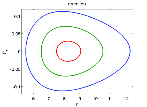
Figure 1: Three Poincaré sections of the phase space trajectories of nonchaotic particle orbits. Each has $L=3.6$ and from the innermost orbit out $E_{1}=0.9499$, $E_{2}=0.9511$, and $E_{3}=0.9534$. Notice that the trajectories are confined to the surface of the tori which intersect the section.

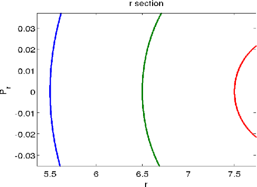
Figure 2: A close up view of the orbits from Fig. 1. Notice that this zoomed in view continues to show the trajectories are constrained to the tori.

When considering sections for spinning test particle orbits we look for this clean oval to break up as in Figure 3. A closer look at the bands (Figure 4 ) clearly shows phase space trajectories have left the torus surface. The orbits that produce sections like this are close in to the black hole and are in agreement with the sections produced by Suzuki1997 .

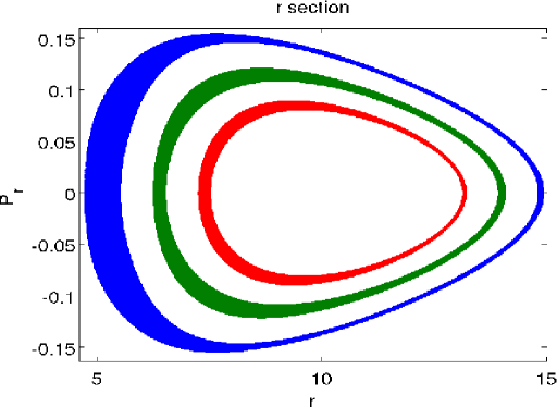
Figure 3: Three Poincaré sections of the phase space trajectories of chaotic particle orbits. From the inside orbit out the orbits have spin values $S_{1}=1.515$ $S_{2}=1.581$ and $S_{3}=1.627$. Notice that the trajectories stay close to the surface of the tori similar to Figure 1, but do not have the thinly defined surface.

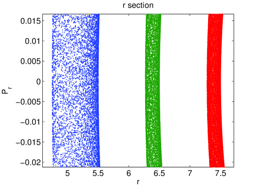
Figure 4: A close up view of the orbits from Fig. 3. Notice that this zoomed in view continues to show the trajectories are not constrained to the tori. Compare to Fig. 2

The second method we use to look for chaos in this system is to calculate Lyapunov exponents. If one defines the distance $D$ between two phase space trajectories as

$$D\left(t\right)=d_{0}e^{\lambda t}$$ (24)

where $d_{0}$ is the initial separation between the two trajectories, then $\lambda$ is defined to be the Lyapunov exponent. When $\lambda$ is greater than zero the system is said to be chaotic. In Hamiltonian systems, of which the Papapetrou equations are an example, the Lyapunov exponent can never be less than zero. A negative exponent would indicate some kind of attractor in the phase space, but these do not appear in conservative systems.

In practice, calculating $\lambda$ is a challenge. The Jacobian method used by Hartl has the advantage of following just one phase space trajectory. The basic idea is that we can track the growth of a vector in the tangent space of the trajectory to compute the Lyapunov exponent (for more detail see Hartl2002 and Hartl2003 ). The equation that dictates the evolution of this vector is

$$\frac{d\boldsymbol{\xi}}{d\tau}={\bf Df\cdot\boldsymbol{\xi}}$$ (25)

where $\boldsymbol{\xi}$ is a vector in the tangent space, and ${\bf Df}$ is the Jacobian matrix of the system.

To understand this method, consider a high dimensional ellipsoid in the phase space defined by some set of initial conditions. As the system evolves away from these initial conditions, this ellipsoid will become warped. However, by virtue of Liouville’s theorem, the phase space volume of this ellipsoid will be conserved. As a result, any axis of the ellipsoid that corresponds to a chaotic coordinate will stretch. This will necessitate that at least one other axis will contract. The system can have more than one chaotic coordinate, but for each chaotic coordinate there must be a nonchaotic coordinate whose value converges at the same rate as the chaotic coordinate’s value diverges. In other words, for every Lyapunov exponent that corresponds to a chaotic axis there is an exponent with the same magnitude but opposite sign.

The Jacobian method finds the largest Lyapunov exponent by evolving a vector, which is defined by the initial conditions of the system, in the tangent space of the phase space. As the system evolves, this vector lines up with the direction of greatest stretching. By considering the magnitude of this vector as a function of the proper time $\tau$, we can then define the largest Lyapunov exponent of the system by

$$\lambda=\lim_{\tau\rightarrow\infty}\,\Bigl{[}{1\over\tau}\,\ln\Bigl{(}\frac{|\boldsymbol{\xi}|}{|\boldsymbol{\xi_{0}}|}\Bigr{)}\,\Bigr{]}$$ (26)

where $\boldsymbol{\xi_{0}}$ denotes the initial tangent vector. As our numerical integrations cannot continue indefinitely, we will, in our calculations, refer to the Lyapunov exponent as a function of $\tau$,

$$\lambda(\tau)=\frac{\ln(|\boldsymbol{\xi}|)}{\tau}$$ (27)

where we have taken $|\boldsymbol{\xi_{0}}|=1$.

For this last analysis we have denoted the magnitude of a vector $\boldsymbol{\xi}$ by $|\boldsymbol{\xi}|$. Recall that this vector lives in the tangent space to the phase space of our physical system. This leads to uncertainty about what norm to use when calculating a vector magnitude. Eckmann Eckmann1985 shows that when calculating Lyapunov exponents, different norms may lead to different values, but the sign of the exponent will not be affected. With this in mind, we use the Euclidean norm for simplicity when calculating vector magnitudes.

This method can be extended to find the Lyapunov exponent corresponding to each axis of the stretching ellipsoid. Hartl implements this extended method Hartl2002 in some cases and shows that the Lyapunov exponents do come in opposite sign pairs for the spinning particle system. His results also indicate that the direction of greatest stretching is not in the direction of any one coordinate or conjugate momentum. Thus, when we find the largest exponent we do not expect it to correspond to a particular coordinate or momentum.

IV Method for Comparing Lyapunov Exponents

Because the Jacobian method requires the Lyapunov exponent to be defined in terms of a limit we can in practice only approximate its value. In previous work, a particular orbit was allowed to evolve for some set amount of time and with the corresponding value of $\lambda(\tau)$ taken as the approximate exponent.

A problem that arises with this method is that different orbits converge to their Lyapunov exponents at different rates. In particular, the Lyapunov exponent for the case $S=0$ approaches zero much more slowly than for any other similar orbit with small, nonzero spin. To address this issue, we have developed a different method which both reduces computation time and predicts the Lyapunov exponent.

Consider the plots of $\lambda(\tau)$ as shown in Figure 5 and Figure 6. These are typical examples of how $\lambda(\tau)$ converges for a zero spin orbit and a nonzero spin orbit respectively. Notice that the functions are modeled well by the fit

$$f(\tau)=a_{1}+\frac{a_{2}}{\tau^{a_{3}}}$$ (28)

where $a_{1}$, $a_{2}$, and $a_{3}$ are constants that are varied until the root mean square error between the fit and $\lambda(\tau)$ is minimized. More explicitly, the constants are varied to minimize

$$err(\tau)=\sum_{i}^{N}\left(a_{1}+\frac{a_{2}}{\tau_{i}^{a_{3}}}-\lambda(\tau_{i})\right)^{2}.$$ (29)

It is then easy to define the RMS error for the fit as

$$RMS=\sqrt{\frac{err}{N}}\;.$$ (30)

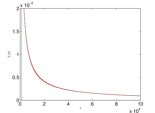
Figure 5: We see the jagged Lyapunov function converging to zero for an orbit with $S=0$. We also plot the curve fit to the data. This orbit begins at $r=6m$ with $P_{\phi}=3.6$. The predicted Lyapunov exponent for this orbit is $-1.68\times 10^{-5}$ with an RMS error of is $1.23\times 10^{-5}$.

The fitting function sets the Lyapunov exponent of the system to be $a_{1}$. Because our system is conservative we cannot have negative Lyapunov exponents. However, in the orbit corresponding to Figure 5 the root mean square error of the fit is $1.23\times 10^{-5}$ while the calculated exponent is nonzero and just a bit outside this error range. Based on other results, such as Figure 6, as well as our method’s consistency with the results of Suzuki1997 and Hartl2002 , we are led to belive that the fit slightly underestimates the Lyapunov exponent. Another example is the orbit corresponding to Figure 6 in which the RMS error is $6.1\times 10^{-5}$ keeping zero well outside the error bars of the fit.

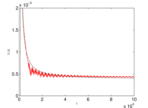
Figure 6: We see the jagged Lyapunov function converging to a nonzero value for an orbit with $S=0.5$. The initial conditions are $r=6m$, $P_{\phi}=3.6$, $\alpha=\frac{\pi}{4}$, and $\beta=\frac{\pi}{4}$. We also plot the curve fit to the data. The predicted Lyapunov exponent is $3.787\times 10^{-4}$ with 0 well outside the RMS error, $6.1\times 10^{-5}$, of the fit.

This model of the Lyapunov function also gives a measure of how quickly the exponent converges. In working with this model we found that orbits with large spin had Lyapunov functions that, in general, converged faster than those with small spin. It is possible that in previous work similar Lyapunov exponents with slower convergence rates might have been discounted as numerical error. The difference in convergence rates between the zero point and these small spin exponents is much smaller than the difference between the zero point and the high spin exponents. If these differing rates of convergence are not taken into account, terminating each orbit after some predetermined time seems natural. Unfortunately, our experience shows that this can inflate the value of the Lyapunov exponent in the zero spin case. Because that case has the slowest rate of convergence, it can then be difficult to distinguish it from cases with nonzero spin and nonzero Lyapunov exponents.

We avoid this problem by comparing Lyapunov exponents once a a uniform degree of convergence has been reached rather than a particular time. While evolving the system we fit the Lyaponv function to Eq. (28) and continue the evolution until the derivative of the fitting function reaches a predefined tolerance close to zero. When the derivative of the fit has become sufficiently small, specifically when the value is on the order of $10^{-8}$, we say that the function has converged. In this way we compare exponents which have all converged the same amount rather than comparing by the overall time of evolution. We find that this method reveals more of the chaotic nature of these orbits.

Further, we can use the fit curve to predict the Lyapunov exponent for a given orbit without integrating for infinite time. These predicted values, together with an estimate of their error, give us confidence that the true exponent is within the corresponding range of values and, more importantly, provide a clear differentiation between positive and zero values.

V Results

A primary motivation for our work is to determine whether or not astrophysically relevant spins can give rise to chaotic orbits. We first consider orbits similar to those considered by Suzuki and Maeda and then look at other types of orbits. Because the orbits considered by Suzuki and Maeda are confined to high curvature regions, the additional orbital types we consider are those that remain in regions of low curvature and orbits that traverse both high and low curvature regions. For each orbital type we begin with a set of initial conditions with $S=0$ and calculate the Lyapunov exponent. We then increase the magnitude of the spin and plot the Lyapunov exponents for each spin.

V.1 High Curvature Orbits

We first consider orbits similar to those used by Suzuki and Maeda Suzuki1997 . These orbits remain close to the center of the spacetime throughout the system’s evolution. This confines the orbits to regions of high curvature which allows the coupling between the curvature and spin to have a large effect on the particle’s motion.

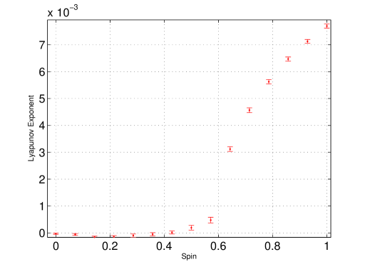
Figure 7: These Lyapunov exponents are given by the constant term in the curve fitting model, Eq. (28), with root mean square error bars. The initial spin orientation is $\alpha=\frac{\pi}{4}$ and $\beta=\frac{\pi}{4}$ and constants of the motion for the spinless case are $L=3.6$ and $E=0.9522$. Compare with Figures 8 and 10. Note that the orbits transition from nonchaotic to chaotic around a spin of $S=0.5$.

One difference between the orbits we consider and those used by Suzuki and Maeda is the orbital angular momentum of the spinning particle. They consider orbits with $L=4.0$ whereas we begin our analysis with orbits having angular momentum of $L=3.6$. Our initial values for energy $E=0.9522$ and an initial radius of $r=6m$ are chosen to make the orbit close to circular. We also keep track of the initial conditions in spin that produce these orbits. In particular, we consider what spin magnitudes produce chaotic orbits and how the spin vector’s initial orientation affects the Lyapunov exponents. In the first case the spin vector’s initial orientation is given by $\alpha=\frac{\pi}{4}$ and $\beta=\frac{\pi}{4}$.

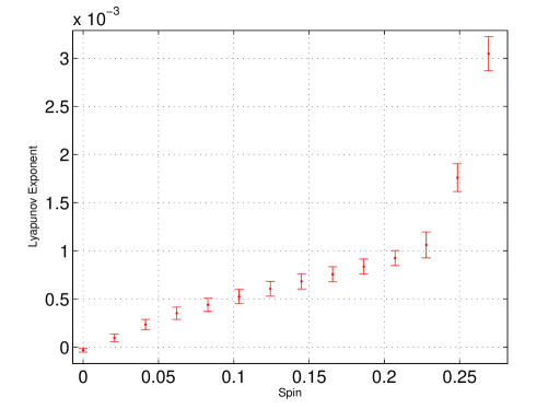
Figure 8: These Lyapunov exponents are given by the constant value in the curve fitting model with the root mean square value providing the error bars. The initial spin orientation is $\beta=\pi$ and constants of the motion for the spinless case are $L=3.6$ and $E=0.9522$. All spin values higher than $S=0.3$ cause the particle to cross the event horizon. Note that lower spin values give exponents of the same order of magnitude as those in Figure 7.

As Figure 7 shows, the Lyapunov values for this orbit can be put into one of two groups. From the maximal spin value of one down to about $S=0.5$ there seems to be a well defined trend with nonzero Lyapunov exponents and corresponding chaotic orbits. These values are in agreement with those reported by Suzuki and Maeda as well as Hartl. From $S=0.5$ down to zero spin the orbits are not chaotic. Again, we find excellent agreement with Suzuki1997 and Hartl2003 .

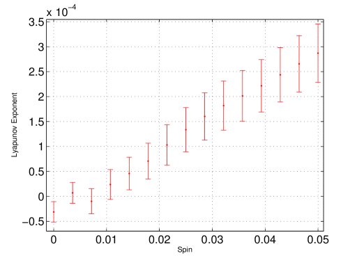
Figure 9: These Lyapunov exponents correspond to the small spin case of Figure 8 with $\beta=\pi$. Note the monotonically decreasing, yet still positive, values of the exponent for decreasing spin values. This trend continues for spins as low as $S=0.015$. However, this trend would appear to be lost for the very smallest values of spin. Indeed, we feel confident to treat these values as zero with correspondingly nonchaotic orbits.

The initial spin vector orientation can affect the magnitude of the Lyapunov exponent. As an example, if we change the spin orientation but otherwise keep the same initial conditions as before, the particle’s behavior changes. When $\beta=\pi$, the spin is pointed down perpendicular to the equatorial plane, the spin orbit coupling causes the particle to be pulled in closer to the center of the spacetime. We find that when the spin angular momentum and orbital angular momentum are parallel there is a repulsive spin orbit interaction and when the momenta are antiparallel there is an attractive interaction. These results agree with Wald’s Wald1972 analysis of similar systems. When this interaction becomes strong enough the particle will no longer exhibit a bound orbit, and is captured by the black hole. In Figure 8 we see the Lyapunov exponent values for increasing spin values. Notice that after $S\approx 0.3$ there is no data. These data points are not included because for $S>0.3$ the particle is captured by the black hole.

Notice also that the exponents in Figure 8 appear to be nonzero below $S=0.05$. Since the interaction between the spin angular momentum and the orbital angular momentum pulls the particle in closer, the particle traverses higher curvature regions of the spacetime than the orbits described by Fig 7. This spin orientation is the only difference between the two cases. Thus, on comparing Figure 7 and Figure 8 we can see that the orientation of the spin can have a dramatic effect on the dynamics of the particle.

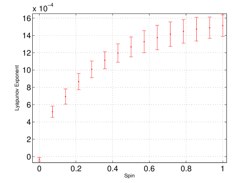
Figure 10: These Lyapunov exponents are given by the constant value in the curve fitting model with the root mean square value providing the error bars. The initial spin orientation is $\beta=0$ and constants of the motion for the spinless case are $L=3.6$ and $E=0.9522$. No large exponents (compare to Figure 7) appear in this configuration.

In Figure 9 we zoom in on the small spin value orbits. This data clearly shows positive Lyapunov exponents for spins as small as $S\approx 0.015$. This lower bound in spin is considerably less than the bounds given in Suzuki1997 and  Hartl2003 . Notice that exponents in Figure 9 are small in comparison to Figure 7. Using our particular fitting method here to predict the Lyapunov exponent was crucial in being ablt to distinguish these small exponents from zero.

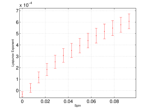
Figure 11: These Lyapunov exponents are given by the constant value in the curve fitting model with the root mean square providing the error bars. The initial spin orientation is $\beta=0$ and constants of the motion for the spinless case are $L=3.6$ and $E=0.9522$. Note that unlike Figure 7 the exponents all appear to be nonzero. No large exponents (compare to Figure 7) appear in this configuration. Note the continuous nature to the exponents and the apparently positive value for spin as low as $S=0.01$.

When we set the initial spin orientation to $\beta=0$, as in Figure 10, the particle is pushed further out from the center instead of pulled closer in. In this case the spin vector and orbital angular momentum vector are parallel. In this case the particle is never captured by the black hole. Instead the particle’s orbit stays in areas of the spacetime with slightly less curvature. Also, the Lyapunov exponents stay at the same order of magnitude as the smaller values from Figure 7 for all spin values, but unlike Figure 7 no nonzero spins correspond to a zero exponent. In Figure 11 we look more closely at the small spin values for the same orbit. We notice the monotinicity in the predicted exponent values, and a nonzero exponent for spin values as low as $S=0.01$.

We also consider orbits which remain in areas of low curvature. Choosing nearly circular orbits at radii of $100m$ and calculating the Lyapunov exponents as above, we find such orbits to have a uniformly zero Lyapunov exponent for every spin orientation which we consider above. When the radii is sufficiently reduced, $r\approx 19m$, positive exponents are again obtained. These positive exponents first occur for very large spin, but as the radius continues to decrease, less spin is required to achieve a chaotic orbit.

V.2 Knife Edge Orbits

Knife edge orbits are some of the more interesting test particle trajectories allowed in black hole spacetimes. These orbits have large scale precession and execute small tight loops around the center of the system. Their dynamics can be understood by considering the effective potential in the Schwarzschild spacetime. For large enough angular momentum this potential has a sharp peak close to the center of the spacetime. These “knife edge” potentials are what give these orbits their particular dynamics. (For more discussion of these orbits see Wheeler .) These orbits are also known as “zoom whirl” orbits; the name being used to describe their behavior, namely they zoom in from large radius and whirl about the center. (For a comprehensive cataloging of these orbits see Levin2008 );

As we consider knife edge orbits for spinning test particles we focus on the geometry surrounding their path. Unlike the orbits we have considered so far, these move through both high and low curvature regions of the spacetime. These orbits start out relatively far from the center of the spacetime, where the curvature is comparatively low. But during the course of their orbits they execute several small orbits in much higher curvature regions. These types of orbits help us determine whether chaotic orbits must remain in high curvature or just pass through them regularly.

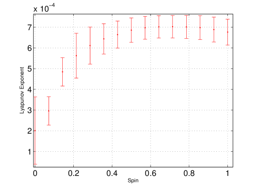
Figure 12: These Lyapunov exponents correspond to knife edge orbits. Notice that the $S=0$ case is very nonzero. This is referred to as a “chaos mimic.” The spinless orbit begins at $r=100m$ and has three inner loops at small radius for each large scale orbit. The initial spin orientation of $\beta=0$. In the spinless case $E=0.997$ and $L=3.9246$.

In Figure 12 we plot the Lyapunov exponents for a knife edge orbit that has an outer radius of $r=100m$ and makes three small radius loops for each large radius orbit. The orientation of the spin is $\beta=0$. The angular momentum of the particle is $L=3.9246$ and which is nearly the angular momentum of the particles investigated by Suzuki and Maeda. We choose this spin orientation to keep the particle from being captured by the black hole. Recall that this orientation gives an effective centrifugal force which pushes the particle away from the black hole. This keeps the particle from being captured, but also reduces the number of inner loops traversed in each orbital period. Thus, as the spin increases, the particle can be thought to be retreating from the knife’s edge.

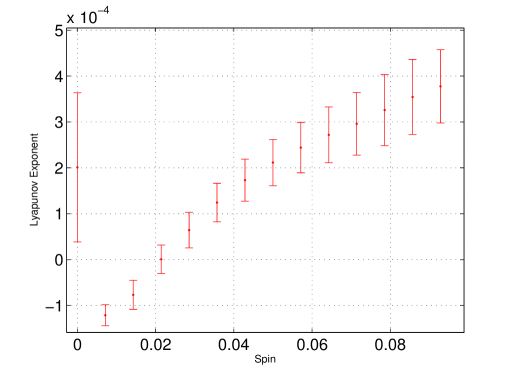
Figure 13: These Lyapunov exponents correspond to the same knife edge orbits as Figure 12. Notice that zero is outside the error bars for spins as low as $S=0.03$.

One important aspect to notice is that the $S=0$ orbit has a drastically nonzero Lyapunov exponent. This effect is referred to as a “chaos mimic” and Hartl finds the same effect for knife edge orbits in the Kerr spacetime Hartl2003 . This effect casts some doubt on the Lyapunov exponents calculated for the nonzero case. Some confidence is restored by the trend in the exponents as the spin decreases, specifically that the values approach zero as spin goes to zero. In Figure 13 we see a close up look at small spin values for the knife edge orbit. We still have the chaos mimic when $S=0$, but we also see a very clear trend in the exponents as the spin decreases.

V.3 Chaotic Orbits With Physical Spin

We now present a particular chaotic orbit at spin values that may be relevant astrophysically. In this case, the constants of the motion are $E=0.9432$ and $L=3.47$ and the spin vector orientation is $\beta=\pi$. These initial conditions define a knife edge orbit which is constrained to regions of high curvature. The effective potential for this orbit is shown in Figure 14. Notice that the potential well confines the particle with $E^{2}=0.8897$, denoted by the dotted line, to remain close to $r=6m$.

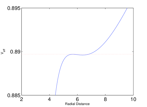
Figure 14: This is a plot of the effective potential corresponding to a knife edge orbit constrained to high curvature regions. This orbit has $L=3.47$ and $E=0.9432$. The line $E^{2}=0.8897$ is shown by the dotted line and shows that the particle is constrained to remain near $r=6m$.

In Figure 15 we see Lyapunov exponents corresponding to this orbit. Similar to Figure 10, spin values greater than those shown on the graph cause the particle to be captured by the black hole. What is more interesting however, is that these nonzero Lyapunov exponents correspond to physical spin values and that these values have comparable magnitude to the larger exponents of Figure 7.

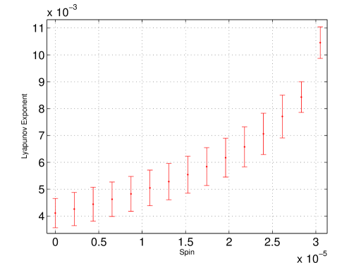
Figure 15: Lyapunov exponents for spin values in the physical range. These orbits have orientation $\beta=\pi$ and constants of the motion for the spinless case are $L=3.47$ and $E=0.9432$. Note the chaos mimic when $S=0$ and the magnitude of the exponent is comparable to the larger values of Figure 7.

One concern with this data is that the exponents seem to converge to the value of the chaos mimic of $S=0$. We can use the KAM tori corresponding to this orbit to resolve this concern. In Figures 16 and 17 we compare the Poincaré sections of this orbit when $S=0$ and equal steps between $S=3.0\times 10^{-5}$ and $S=3.069\times 10^{-5}$ respectively.

Notice that when $S=0$ the phase space trajectory is confined to the surface of the 2 torus intersected by the $r-P_{r}$ plane. We can see this detail in the upper right of Figure 17. In the nonzero spin cases the same Figure shows the breaking up of the tori surfaces which is indicative of chaos. Based on the positive indication for chaos given by both the Lyapunov exponent and the Poincaré sections we conclude that this orbit is indeed chaotic for some initial conditions that correspond to astrophysically realizable amounts of spin.

As the spin decreases from $S=3.069\times 10^{-5}$ the breaking of the torus becomes less and disappears by $2.8\times 10^{-5}$. Thus, it would appear that the points of Figure 15 with smaller spins than this amount are not truly chaotic. Since these first points seem to converge to the chaos mimic of the $S=0$ case it is likely that the positive exponents corresponding to unbroken tori are inflated by the chaos mimic exactly as in the zero spin case. We notice from the graph that the final point has smaller error bars than the previous points. Because this orbit is shown to be chaotic by its Poincaré section, the true chaotic behavior of the particle may push it above the exponent magnitude created by the chaos mimic.

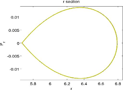
Figure 16: These are Poincaré sections in the $r-P_{r}$ plane for $S=0$ and five orbits with spin magnitudes spaced equally from $S=3.0\times 10^{-5}$ to $S=3.069\times 10^{-5}$. These orbits have the orientation $\beta=\pi$ and constants of the motion for the spinless case are $L=3.47$ and $E=0.9432$. Notice that unlike Figures 1 and 3 the initial conditions of the orbits make them difficult to distinguish at this level.

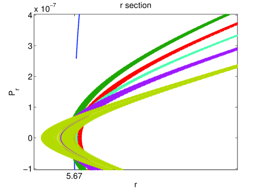
Figure 17: This is a closer look at Fig. 16. The point $r=5.67$ is marked on the axis which spans $r=5.67-1\times 10^{-6}$ to $r=5.67+3.5\times 10^{-6}$. This finer line in the upper left is the part of the section for the spinless case. Notice the distinct breaking of the tori for the other five orbits. These orbits increase in spin from top to bottom of the upper right corner.

VI Conclusion

We find that chaotic orbits with apparently astrophysically relevant spins do exist in the Schwarszchild spacetime. In particular, we have shown that for a spin values between $S=3.0\times 10^{-5}$ and $S=3.069\times 10^{-5}$ both the Lyapunov exponent and the Poincaré section indicate a chaotic orbit. Recall that Hartl’s Hartl2003 bounds for chaotic spin values were $10^{-4}$ to $10^{-6}$. These orbits combine the dynamics of knife edge orbits with the high curvature close to the center of the spacetime. While this is a special class of orbit, decaying orbits may exhibit this behavior before they are captured by the black hole. Indeed, Levin Levin2000 has shown that compact binaries pass through a chaotic region when inspiraling and it is an interesting question as to whether decaying orbits could pass through these astrophysical, chaotic orbits.

The results of our analysis also put the cutoff spin value for chaotic orbits much lower than previously thought even for more general orbits. Suzuki and Maeda Suzuki1997 give a cutoff value of about $S=0.63$ when the orbital angular momentum of the particle is $L=4$. We have provided strong numerical evidence that chaotic orbits exist for spin values less than $S=0.01$ for orbits with $L=3.6$.

Both Suzuki1997 and Hartl2003 claim that the spin-spin interaction in the Kerr metric results in an even greater number of chaotic orbits with small spin than in the Schwarzschild spacetime considered here. Indeed, Hartl found a lower bound for spins that yield chaotic orbits of about $S=0.1$. As the knife edge orbits that we have investigated here also exist in modified form in the Kerr spacetime, we might expect that there are even more chaotic orbits with physically relevant spins in Kerr.

A final important question, which is the subject of Suzuki1999 ; Kiuchi2004 , is the potential impact of these chaotic orbits on the gravitational wave emission from these systems. Certainly, the current results are suggestive that there is a chaotic regime in spin which might be astrophysically accessible to extreme mass-ratio binaries. If so, then gravitational waves emitted by binary systems with large mass ratios might contain this chaotic imprint. Thus, analyzing these systems for gravitational wave emission would be a natural next step in understanding chaos in these systems.

- (1) T. Tanaka, Jour. Phy. Conf. Series 120, 032001 (2008)
- (2) R. Hojman and S. Hojman, Phys. Rev. D 15, 2724 (1977)
- (3) O. Semerák, Mon. Not. R. Astron. Soc. 308, 863 (April 1999)
- (4) S. Suzuki and K. Maeda, Phys. Rev. D 55, 4848 (April 1997)
- (5) M. D. Hartl, Phys. Rev. D 67, 024005 (January 2003)
- (6) M. D. Hartl, Phys. Rev. D 67, 104023 (May 2003)
- (7) S. Suzuki and K. Maeda, Phys. Rev. D 61 (December 1999)
- (8) K. Kiuchi and K. Maeda, Phys. Rev. D 70 (September 2004)
- (9) N. J. Cornish, Phys. Rev. D 64, 084011 (September 2001)
- (10) A. Papapetrou, Proc. Roy. Soc. 209, 248 (1951)
- (11) W. G. Dixon, Nuovo Cim. 34, 317 (1964)
- (12) W. G. Dixon, Proc. Roy. Soc. Lond. 314, 499 (1970)
- (13) J. Ehlers and E. Rudolph, Gen. Rel. Grav. 8, 197 (1977)
- (14) There are differences in sign with Hartl’s definitions. The reason is he makes the change of variables which changes the handedness of his coordinate system. This in turn affects the overall sign of
- (15) R. C. Hilborn, Chaos and Nonlinear Dynamics, 2nd ed. (Oxford University Press, 2000)
- (16) E. Ott, Chaos in Dynamical Systems, 2nd ed. (Cambridge University Press, 2002)
- (17) J. Eckmann and D. Ruelle, Rev. Mod. Phys. 57, 617 (July 1985)
- (18) R. M. Wald, Phys. Rev. D 6, 406 (July 1972)
- (19) As far as we can tell, this term was first used by Ruffini and Wheeler in The Significance of Space Research for Fundamental Physics in 1970.
- (20) E. F. Taylor and J. A. Wheeler, Exploring Black Holes (Addison Wesley Longman, 2000)
- (21) J. Levin and G. Perez-Giz, Phys. Rev. D 77 (May 2008)
- (22) These chaos mimics have positive Lyapunov exponent due to the dynamics of knife edge orbits. The combination of large and small radius orbits causes to grow very large. Interestingly, the effects causing the mimics can be lessened, and sometimes removed, by using the geodesic equation in contravariant form as the particle’s equations of motion. Unfortunately, the chaos mimic that appears in the physical chaotic orbit cannot be removed by making this change.
- (23) J. Levin, Phys. Rev. Lett. 84, 3515 (April 2000)