Photon Distribution Amplitudes in nonlocal chiral quark model

Abstract

Photon distribution amplitudes up to twist four are calculated within the nonlocal chiral quark model with a simple pole ansatz for momentum dependence of the constituent quark mass. Calculations are performed using modified electromagnetic vector current in order to satisfy Ward identities. Quark condensate and magnetic susceptibility of the QCD vacuum entering definitions of the distribution amplitudes are computed and compared with existing phenomenological estimates. Both real and off-shell photons are considered and relevant form factors are calculated. Our results are analytical up to the numerical solution of certain algebraic equation.

I Introduction

In the present paper we calculate photon distribution amplitudes (DA) within a low energy nonlocal model based on the instanton model of the QCD vacuum. There are seven different photon DAs corresponding to the Dirac structure probing the photon and to the light-cone twist (here we follow closely definitions of ref. Ball:2002ps ). However in reality only one of them, twist 2 tensor DA, can be accessed experimentally in hard exclusive processes Braun:2002en ; Rohrwild:2007yt ; Pire ; Szymanowski:2009tc (for experimental overview see ref. Ashery:2006zw ). Higher twist amplitudes are suppressed in hard processes and vector twist 2 DA decouples for real photons. However, the interest in the remaining photon DAs is not purely academical. They are normalized through low energy observables such as quark condensate – $\left\langle\bar{\psi}\psi\right\rangle$, magnetic susceptibility – $\chi_{m}$ and mixed quark-gluon condensate – $f_{3\gamma}$ that are of importance for our understanding of the properties of the QCD vacuum. Only the calculation of all photon DAs provides a test of the whole approach and may prove its consistency.

In the present work we employ a nonlocal generalization of the semibosonized Nambu Jona-Lasinio (NJL) model with momentum dependent constituent quark mass $M(p)$ (which will be denoted as $M_{p}$) which follows from the instanton model of the QCD vacuum Diakonov:1983hh ; Shuryak:1984kp . This model in the present version has been previously used to calculate pion Praszalowicz:2001wy ; Praszalowicz:2001pi ; Bzdak:2003qe and kaon Nam:2006au ; Nam:2006mb ; Nam:2006sx distribution amplitudes, two pion DAs Praszalowicz:2003pr , pion-to-photon transition distribution amplitudes Kotko:2008gy and also twist 2 tensor photon DA Petrov:1998kg (see also Praszalowicz:2001wy ). However a complete analysis of all seven photon DAs has been, to the best of our knowledge, conducted only in ref. Dorokhov:2006qm in a model similar to ours with, however, results that in some respects are different than the ones obtained in the present paper.

One of the obvious problems that arises when one considers momentum dependent fermion mass is the nonconservation of the naive vector current containing only $\gamma^{\mu}$ Dirac matrix. There are many proposals in the literature how to extend vector current to satisfy electromagnetic Ward identities. None of them is unique, since current conservation does not fix the transverse part of the modified vertex. One of the simplest extensions of this type discussed already many years ago in refs. Ball:1980ay ; Frank:1994gc and employed also in ref. Dorokhov:2006qm , consists in the following substitution

$$\gamma^{\mu}\rightarrow\gamma^{\mu}-\frac{k^{\mu}+(k-p)^{\mu}}{k^{2}-(k-p)^{2}}\left(M_{k}-M_{k-p}\right).$$ (1)

Extension (1) follows from the assumption concerning both Ward identities and analytical structure of the modified vertex that is required to match perturbative expansion. In principle one could add to (1) terms proportional to $r^{\mu}$ where $r\cdot p=0$, and the Ward identities would be satisfied. In refs. Bowler:1994ir ; Plant:1997jr and also in Broniowski:1999bz another modification has been advocated; here the ambiguity is connected to a freedom of choosing the integration path that defines the nonlocal vertex. In view of this ambiguous situation we have decided to use the simplest possible extension of ref. Ball:1980ay given by eq. (1).

Unlike the pion or the $\rho$ meson the photon has a dual nature being both point-like and composite at the same time. Therefore in order to calculate photon DAs that describe nonperturbative quark-antiquark structures, one has to subtract the perturbative part. In order to avoid ambiguities this procedure has to be well defined. In our case, since we work in the chiral limit, we subtract the perturbative part only from these photon DAs that are nonzero for massless quarks. These are: vector and axial DAs which are also UV divergent. Therefore the subtraction of the perturbative part renormalizes these DAs ensuring their finiteness. At the same time it introduces a term proportional to $\ln(-P^{2})$ that develops imaginary part for positive virtualities. This is the reflection of the fact that the photon can decay into free massless quarks in the chirally even channels. Throughout this paper we plot DAs both for negative and positive photon virtualities, in the latter case we take just the real part if the imaginary part exists. We also display momentum dependence of the pertinent decay constants that are characterized by dimensionless functions $F_{T,V,A}(P^{2})$ for brevity referred to as form factors.

Finally let us make a technical remark concerning loop integrals over $d^{4}k$ with $k^{+}=uP^{+}$ component fixed by the $\delta$ function. Such integrals, depending on the tensor structure may contain "singular" pieces proportional to $\delta(u)$ and $\delta(u-1)$ or even the derivatives of the $\delta$ functions. This is the case for higher twist photon DAs only. We discuss this in more detail in sect. IV, here we just want to point out that higher twist DAs are in fact distributions rather than ordinary functions. Quite importantly, the $\delta$ function contribution is always accompanied by a regular piece that together with the $\delta$ piece integrates to zero for any $P^{2}$. This allows to define a properly normalized regular part and a singular part of DA of zero norm.

In the next section we introduce kinematical variables and define photon distribution amplitudes. In sect. III we describe the main features of our model specifying the ansatz for the momentum dependence of the constituent quark mass. We fix model parameters requiring that the experimental value of the pion decay constant $F_{\pi}=93$ MeV is reproduced. To this end we use model formula given in eq. (18). Next, in sect. IV, we describe techniques used to calculate loop integrals with momentum dependent constituent quark mass. We pay special attention to Lorentz invariance and show how the end point singularities proportional to the Dirac $\delta$ functions arise. Main results are presented in sect. V. First we calculate dimensional constants entering definitions of the DAs (7)–(9), namely quark condensate, magnetic susceptibility and yet another constant, called $f_{3\gamma}$. We obtain numerical results that agree with the "experimental" values known from phenomenology. Finally in sections V.1 and V.2 we present our main results plotting different DAs and discussing their properties.

Our results can be briefly summarized as follows. Leading twist amplitudes are rather insensitive to model parameters, whereas higher twist amplitudes exhibit much stronger dependence, moreover some of them contain $\delta$ functions. We also show the influence of the nonlocal part of the photon vertex (1) on the shape of photon DAs. For some DAs it is rather unimportant, for the other ones it is absolutely crucial. More discussion and comparison with other models is given in sect. VI. Technical details are collected in appendices.

II Definitions and kinematics

Photon distribution amplitudes are defined through matrix elements of the nonlocal quark-antiquark billinears between vacuum and one photon state. Quark operators are assumed to be on the light cone separated by the distance $2\lambda$. In the following we use the light-cone coordinates defined by two light like vectors $n^{\mu}$ and $\tilde{n}^{\mu}$ such that $n^{\mu}=\left(1,0,0,-1\right)$ and $\tilde{n}^{\mu}=\left(1,0,0,1\right)$. In this basis any four-vector $v^{\mu}$ can be decomposed into $v^{+}$ and $v^{-}$ components

$$v^{\mu}=v^{+}\frac{\tilde{n}^{\mu}}{2}+v^{-}\frac{n^{\mu}}{2}+v_{\bot}^{\mu}.$$ (2)

Scalar product can be written as

$$u\cdot v=\frac{1}{2}u^{+}v^{-}+\frac{1}{2}u^{-}v^{+}-\vec{u}_{\bot}\cdot\vec{v}_{\bot}.$$ (3)

We shall work in the system where the photon momentum is expressed as

$$P^{\mu}=P^{+}\frac{\tilde{n}^{\mu}}{2}+\frac{P^{2}}{P^{+}}\frac{n^{\mu}}{2}.$$ (4)

Decomposition of the polarization vector reads

$$\varepsilon^{\mu}=\varepsilon^{+}\frac{\tilde{n}^{\mu}}{2}+\varepsilon^{-}\frac{n^{\mu}}{2}+\varepsilon_{\bot}^{\mu},\quad\text{where}\quad\varepsilon_{\bot}^{\mu}\varepsilon_{\bot\,\mu}=-\vec{\varepsilon}_{\bot}\cdot\vec{\varepsilon}_{\bot}=-1.$$ (5)

Since $P\cdot\varepsilon=0$ we have the relation

$$\varepsilon^{-}=-\frac{P^{2}}{\left(P^{+}\right)^{2}}\varepsilon^{+}.$$ (6)

For real photon we obviously have $\varepsilon^{+}=\varepsilon\cdot n=0$ and consequently $\varepsilon^{-}=0$ as well.

Depending on different tensor nature of the bilocal operators, we can define tensor

$$\left\langle 0\left|\overline{\psi}\left(\lambda n\right)\sigma^{\alpha\beta}\psi\left(-\lambda n\right)\right|\gamma\left(P,\varepsilon\right)\right\rangle =i\frac{e}{2}\left\langle\bar{\psi}\psi\right\rangle F_{T}\left(P^{2}\right)$$

$$\Bigg{\{}\left(\varepsilon_{\bot}^{\alpha}\tilde{n}^{\beta}-\varepsilon_{\bot}^{\beta}\tilde{n}^{\alpha}\right)P^{+}\chi_{m}\int_{0}^{1}du\,e^{i\xi\lambda P^{+}}\,\phi_{T}\left(u,P^{2}\right)$$

$$\frac{1}{P^{+}}\left(\tilde{n}^{\alpha}n^{\beta}-\tilde{n}^{\beta}n^{\alpha}\right)\varepsilon^{+}\,\int_{0}^{1}du\,e^{i\xi\lambda P^{+}}\,\psi_{T}\left(u,P^{2}\right)$$

$$\frac{1}{P^{+}}\left(\varepsilon_{\bot}^{\alpha}n^{\beta}-\varepsilon_{\bot}^{\beta}n^{\alpha}\right)\int_{0}^{1}du\,e^{i\xi\lambda P^{+}}\,h_{T}\left(u,P^{2}\right)\Bigg{\}}$$ (7)

vector

$$\left\langle 0\left|\overline{\psi}\left(\lambda n\right)\gamma^{\mu}\psi\left(-\lambda n\right)\right|\gamma\left(P,\varepsilon\right)\right\rangle =ef_{3\gamma}F_{V}\left(P^{2}\right)$$

$$\Bigg{\{}\frac{1}{2}\tilde{n}^{\mu}\varepsilon^{+}\int_{0}^{1}du\,e^{i\xi\lambda P^{+}}\,\phi_{V}\left(u,P^{2}\right)$$

$$+\varepsilon_{\bot}^{\mu}\,\int_{0}^{1}du\,e^{i\xi\lambda P^{+}}\,\psi_{V}\left(u,P^{2}\right)$$

$$-\frac{1}{2}\frac{P^{2}}{\left(P^{+}\right)^{2}}n^{\mu}\varepsilon^{+}\int_{0}^{1}du\,e^{i\xi\lambda P^{+}}\,h_{V}\left(u,P^{2}\right)\Bigg{\}}$$ (8)

and axial vector

$$\left\langle 0\left|\overline{\psi}\left(\lambda n\right)\gamma^{\mu}\gamma_{5}\psi\left(-\lambda n\right)\right|\gamma\left(P,\varepsilon\right)\right\rangle =\frac{1}{2}ef_{3\gamma}F_{A}\left(P^{2}\right)$$

$$\epsilon_{\mu\nu\alpha\beta}\varepsilon_{\bot}^{\nu}\tilde{n}^{\alpha}n^{\beta}P^{+}\lambda\int_{0}^{1}du\,e^{i\xi\lambda P^{+}}\psi_{A}\left(u,P^{2}\right)$$ (9)

distribution amplitudes. For compactness we used notation $\xi=2u-1$ where $u$ is longitudinal fraction of the quark momentum and dropped Wilson lines $\left[-\lambda n,\lambda n\right]$ that ensure gauge invariance of the nonlocal operators. In the light-cone gauge $A\cdot n=0$ and hence $\left[-\lambda n,\lambda n\right]=1$. Moreover, since we use an effective model where gluonic fields are integrated out, Wilson lines corresponding to gluon fields never appear.

Our definitions follow closely those of refs.  Ball:2002ps and Dorokhov:2006qm , however we need only one $P^{2}-$dependent dimensionless form factor for each tensor structure: $F_{T}\left(P^{2}\right)$, $F_{V}\left(P^{2}\right)$ and $F_{A}\left(P^{2}\right)$ where subscripts $T,\,V$ and $A$ stay for vector, tensor and axial vector, respectively. Constant $\chi_{m}$ is the magnetic susceptibility of the quark condensate $\left\langle\bar{\psi}\psi\right\rangle$, and $f_{3\gamma}$ corresponds to the axial mixed quark-gluon condensate. They provide natural mass scales for distribution amplitudes. Analytical expressions for $\left\langle\bar{\psi}\psi\right\rangle$, $\chi_{m}$ and $f_{3\gamma}$, and for the form factors can be retrieved from the matrix elements of local operators:

$$\left\langle 0\left|\overline{\psi}\left(0\right)\sigma^{\alpha\beta}\psi\left(0\right)\right|\gamma\left(P,\varepsilon\right)\right\rangle =ie\left\langle\bar{\psi}\psi\right\rangle\chi_{m}F_{T}\left(P^{2}\right)\left(\varepsilon^{\alpha}P^{\beta}-\varepsilon^{\beta}P^{\alpha}\right),$$ (10)

$$\left\langle 0\left|\overline{\psi}\left(0\right)\gamma^{\mu}\psi\left(0\right)\right|\gamma\left(P,\varepsilon\right)\right\rangle =ef_{3\gamma}F_{V}\left(P^{2}\right)\varepsilon^{\mu},$$ (11)

$$\left.\frac{d}{d\lambda}\left\langle 0\left|\overline{\psi}\left(-\lambda n\right)\gamma^{\mu}\gamma_{5}\psi\left(\lambda n\right)\right|\gamma\left(P,\varepsilon\right)\right\rangle\right|_{\lambda=0} =ef_{3\gamma}F_{A}\left(P^{2}\right)\epsilon_{\mu\nu\alpha\beta}\varepsilon^{\nu}P^{\alpha}n^{\beta}.$$ (12)

Equations (7)-(9) define photon distribution amplitudes that can be classified according to the kinematical light-cone twist. We have distributions of twist-2: $\phi_{T}$, $\phi_{V}$, of twist-3: $\psi_{T}$, $\psi_{V}$, $\psi_{A}$ and of twist-4: $h_{T}$, $h_{V}$. This can be easily seen by inspecting eqs. (7)-(9), since the twist counting actually reduces to counting the powers of $P^{+}$. Notice that in the case of axial distribution the power of $P^{+}$ equals $1$, what would correspond to twist-2, however additionally there is a path stretch $\lambda$ with inverse mass dimensionality that makes $\psi_{A}$ to have twist 3 rather than 2.

Constants $\chi_{m}$, $\left\langle\bar{\psi}\psi\right\rangle$ and $f_{3\gamma}$ are chosen in such a way that the following normalization conditions are satisfied

$$\int_{0}^{1}\,\phi_{T}\left(u,P^{2}\right)du =1,\quad\int_{0}^{1}\,\psi_{T}\left(u,P^{2}\right)du=\chi_{m}P^{2},\quad\int_{0}^{1}\,h_{T}\left(u,P^{2}\right)du=\chi_{m}P^{2},$$ (13)

$$\int_{0}^{1}\,\phi_{V}\left(u,P^{2}\right)du =1,\quad\quad\int_{0}^{1}\,\psi_{V}\left(u,P^{2}\right)du=1,\quad\quad\quad\int_{0}^{1}\,h_{V}\left(u,P^{2}\right)du=1$$ (14)

$$\quad\int_{0}^{1}\,\psi_{A}\left(u,P^{2}\right)du=1.\quad$$ (15)

Note that due to the conservation of vector current $F_{V}(0)=0$. On the other hand $F_{T}(0)=1$. Normalization of the axial form factor $F_{A}(0)$ is arbitrary and depends on the dimensional constant used in definition (9).

III Nonlocal chiral quark model

In order to calculate relevant matrix elements in the low energy domain we shall use effective action based on the instanton vacuum theory Diakonov:1983hh . Its main feature is momentum dependent constituent quark mass

$$M\left(k\right)=M\,F^{2}\left(k\right)$$ (16)

appearing due to the chiral symmetry breaking. This dependence enters not only into propagators, but serves as a nonlocal quark-meson coupling as well. For zero momentum $M\left(0\right)\equiv M$ is of order of $350\,\mathrm{MeV}$, while for $k\rightarrow\infty$ constituent quark mass vanishes $M\left(k\right)\rightarrow 0$.

One has to remember that the semibosonized NJL model, although devised to describe chiral physics of Goldstone bosons, has been widely used to incorporate baryons as chiral solitons both in local (for review see e.g. ref. Christov ) and non-local RipBroGo cases. Generally the results of these studies show that the soliton ceases to exist for too small constituent quark mass $M$. The critical value of $M$ depends on the details of the given model, however it is of the order of 300 MeV or a bit less. Typical values of $M$ that fit well the hyperon spectrum may be as high as 420 MeV Blotzetal . In order to investigate dependence of photon DAs on $M$ we use three distinct values of $M$: 300, 350 and 400 MeV.

Due to the momentum dependence of the quark mass, the naive vector current $j^{\mu}=\bar{\psi}\gamma^{\mu}\psi$ violates electromagnetic Ward identities. In order to fix this deficiency new nonlocal terms have to be added to $j^{\mu}$. As already discussed in the Introduction there are several ways of constructing extensions that make the current conserved. In the present paper we use the simplest possible generalization of the vector current, Ball:1980ay ; Dorokhov:2006qm replacing $\gamma^{\mu}$ by an effective vertex of (1). One can easily check that electromagnetic Ward identities are satisfied when (1) is used instead of $\gamma^{\mu}$. Although eq. (1) introduces an extra pole inside Feynman amplitudes, its residue, as we will explicitly show, is zero due to the mass difference in the numerator. This generalization of the vector current has been widely used in the literature also in the context of the photon DAs Dorokhov:2006qm .

Expression for the form factor $F_{\mathrm{inst}}\left(k\right)$ within instanton vacuum model is known analytically in Euclidean space and is highly nontrivial Diakonov:1983hh . Therefore, in order to perform analytical calculations directly in Minkowski space, we use the following formula Praszalowicz:2001wy

$$F(k)=\left(\frac{-\Lambda_{n}^{2}}{k^{2}-\Lambda_{n}^{2}+i\epsilon}\right)^{n},$$ (17)

where $\Lambda_{n}$ is cutoff parameter adjusted for each $n$ in such a way, that the experimental value of the pion decay constant is reproduced. For transparency we shall skip subscript $n$ and use $\Lambda$ rather than $\Lambda_{n}$ in the following.

Equation (17) reproduces reasonably well original shape $F_{\mathrm{inst}}\left(k\right)$ when continued to Euclidean momentum. It should be however pointed out that expression (17) does not follow the exponential asymptotics of $F_{\mathrm{inst}}\left(k\right)$ Diakonov:1983hh . Parameter $n$ is introduced in order to check sensitivity of our results to the shape of $F\left(k\right)$.

In order to fix the model parameter $\Lambda$ we use the following Euclidean expression for the weak pion decay constant Bowler:1994ir :

$$F_{\pi}^{2}=\frac{N_{c}}{4\pi^{2}}\int_{0}^{\infty}dk_{\mathrm{E}}^{2}\,k_{\mathrm{E}}^{2}\frac{M^{2}\left(k^{2}_{\mathrm{E}}\right)-k_{\mathrm{E}}^{2}M\left(k^{2}_{\mathrm{E}}\right)M^{\prime}\left(k^{2}_{\mathrm{E}}\right)+k_{\mathrm{E}}^{4}M^{\prime}\left(k^{2}_{\mathrm{E}}\right)^{2}}{\left(k_{\mathrm{E}}^{2}+M^{2}\left(k^{2}_{\mathrm{E}}\right)\right)^{2}}$$ (18)

where $M^{\prime}(k^{2}_{\mathrm{E}})=dM(k^{2}_{\mathrm{E}})/dk^{2}_{\mathrm{E}}$. Notice that this formula differs from the Pagels-Stokar formula of ref.  Pagels:1979hd . It has been also obtained in ref.  Bzdak:2003qe from the PCAC relation in Minkowski space. Using experimental value $F_{\pi}=93\,\mathrm{MeV}$ and (17) we obtain cutoff parameters listed in Table 1 for several choices of the constituent quark mass $M$ and $n$. Analytical expression obtained within the present model is given in appendix B. We remark at this point that the cutoff parameter $\Lambda$ should not be confused with a typical scale of the model, which for the instanton model is about $600\,\mathrm{MeV}.$

$M=300\,\mathrm{MeV}$
$n=1$	$\Lambda=1016\,\mathrm{MeV}$
$n=5$	$\Lambda=2385\,\mathrm{MeV}$
$M=350\,\mathrm{MeV}$
$n=1$	$\Lambda=836\,\mathrm{MeV}$
$n=5$	$\Lambda=1970\,\mathrm{MeV}$
$M=400\,\mathrm{MeV}$
$n=1$	$\Lambda=721\,\mathrm{MeV}$
$n=5$	$\Lambda=1704\,\mathrm{MeV}$

Table 1: Numerical values of the model parameters obtained using Birse-Bowler formula for pion decay constant $F_{\pi}$.

IV Loop integrals with momentum dependent mass

In this section we present a brief sketch of our calculations underlying the most important steps. Further technicalities are relegated to appendices. In order to calculate the DA of interest – denoted generically as $f(u)$ – we have to invert formulae (7)–(9) by contracting them with appropriate 4-vectors and by performing Fourier transform in $\lambda$. This results in the following formulae

$$f(u)=\frac{-ie_{q}4P^{+}N_{c}}{C}\int\frac{d^{D}k}{\left(2\pi\right)^{D}}\emph{T}_{\Gamma}(k,k-P)\,\delta(k^{+}-uP^{+})$$ (19)

where $C$ is the constant obtained by the contraction, $\Gamma$ is the contracted tensor structure defining given amplitude and

$$\emph{T}_{\Gamma}^{\,}(k,q)=\frac{1}{4}\operatorname{Tr}\left\{\Gamma\frac{1}{\not k-M_{k}+i\epsilon}\,\varepsilon_{\mu}\tilde{\gamma}^{\mu}\left(k,k-P\right)\frac{1}{(\not k-\not P)-M_{k-P}+i\epsilon}\right\}$$ (20)

stands for the Dirac trace. Note that in the case of axial DA, because of $\lambda$ standing in the l.h.s. of (9)

$$f(u)=\frac{1}{2}\left(\psi_{A}^{\prime}(u)+\psi_{A}(0)\delta(u)-\psi_{A}\delta(u-1)\right).$$ (21)

Since some of the integrals can be UV divergent we shall work in $D=4-2\epsilon$ dimensions.

Previous calculations using present nonlocal model were done by integration in the light-cone coordinates, with special care concerning the integration contour to ensure analyticity in $\Lambda_{n}$. Here we present another method of performing such integrals based on the $\alpha$-representation for the propagators. It is especially useful in the case of integrals appearing in higher twist distributions, because of the end point delta-type singularities, which are cumbersome to treat by integration in the light-cone coordinates.

The above complication can be well illustrated by considering a loop integral of the type (19) for the numerator involving $k^{\mu}$. If not for the $\delta$ function it would have been proportional to $P^{\mu},$ but because $k^{+}-uP^{+}=n\cdot k-u\,n\cdot P$ we have

$$\int\frac{d^{D}k}{\left(2\pi\right)^{D}}\frac{k^{\mu}\,\mathcal{N}\,}{\left(k^{2}-M_{k}^{2}+i\epsilon\right)\left(\left(k-P\right)^{2}-M_{k-P}^{2}+i\epsilon\right)}\delta(k^{+}-uP^{+})\,=A(u)P^{\mu}+B(u)n^{\mu}$$ (22)

where $\mathcal{N}$ is some scalar function involving $n$, $\varepsilon$ and $P$. There is an obvious condition following from Lorentz invariance

$${\displaystyle\int\limits_{0}^{1}}duB(u)=0.$$ (23)

However, as mentioned above and as shown explicitly in appendix C function $B(u)$ contains both regular piece and the piece with delta functions: $\delta(u)$ and $\delta(u-1)$. Only the sum of both contributions integrates over $du$ to zero. Note that this cancelation occurs for any $P^{2}$. Since $n\cdot n=0$ and $\varepsilon_{\bot}\cdot n=0$, the delta functions contribute only to the integrals of the $k^{-}$ component. The integrals with tensor structure $k^{\mu}k^{\nu}$ are even more complicated, since they involve derivatives of $\delta$ functions.

As it was already discussed in ref.  Praszalowicz:2001wy momentum mass dependence given by (17) introduces a set of poles, whose positions depend on parameter $\Lambda$. To this end it is convenient to introduce dimensionless scaled variables

$$\kappa=k/\Lambda_{n},\qquad p=P/\Lambda_{n},\qquad r=M/\Lambda_{n}$$ (24)

and to define

$$z_{1}=\left(\kappa-p\right)^{2}-1+i\epsilon,\;z_{2}=\kappa^{2}-1+i\epsilon.$$ (25)

Then the loop integral involving two propagators, like the one in. eq. (22), is transformed into

$$\mathcal{I}=\Lambda^{D-5}\int\frac{d^{D}\kappa}{\left(2\pi\right)^{D}}\,\delta\left(\kappa\cdot n-up^{+}\right)\frac{z_{1}^{4n}z_{2}^{4n}\mathcal{N}}{G\left(z_{1}\right)G\left(z_{2}\right)},$$ (26)

where the numerator $\mathcal{N}(z_{1},z_{2},\kappa\cdot n,\kappa\cdot\tilde{n},\kappa\cdot\varepsilon_{\bot})$ depends on the DA considered. Here

$$G\left(z_{i}\right)=z_{i}^{4n+1}+z_{i}^{4n}-r^{2}=\prod_{j=1}^{4n+1}\left(z_{i}-\eta_{j}\right)$$ (27)

corresponds to the propagator with momentum dependent mass (for $n=0$ it reduces to the ordinary propagator in scaled variables) where the complex numbers $\eta_{j}$ are roots of polynomial $G$ to be obtained numerically.

Next we decompose the inverse product of $G\left(z_{1}\right)G\left(z_{2}\right)$ into a sum of simple poles

$$\frac{z_{1}^{M}z_{2}^{N}}{G\left(z_{1}\right)G\left(z_{2}\right)}=\sum_{i,j=1}^{4n+1}f_{i}f_{j}\frac{\eta_{i}^{M}\eta_{j}^{N}}{(z_{1}-\eta_{i})(z_{2}-\eta_{j})}\;\text{for}\;M,N\leq 4n$$ (28)

with

$$f_{i}=\prod_{k=1,\,k\not=i}^{4n+1}\frac{1}{\eta_{i}-\eta_{k}}.$$ (29)

In this way integral (26) is reduced to the sum of contributions involving two propagators only. It is convenient to use the $\alpha$-representation (exponential Schwinger representation) for the product of propagators since also the $\delta$ function in (26) can be written as an exponent. Further calculations are rather standard and are summarized in appendix C. As a result we obtain analytical expressions given as sums over roots $\eta_{i}$. Certain simplifications occur when we use the following identity (which is true for any set of complex numbers $\{\eta_{i}\}$ not only for the solutions of $G(\eta_{i})=0$):

$$\sum_{i=1}^{4n+1}f_{i}\eta_{i}^{N}=\begin{cases}0&N<4n,\\ 1&N=4n.\end{cases}$$ (30)

The proof of (30) and other useful identities can be found in appendix A.

Some of the loop diagrams discussed above are UV divergent and require renormalization. This results in the subtraction of the perturbative part which is uninteresting from the point of view of the hadronic component of the photon. To illustrate this problem consider loop integral (26) with $\mathcal{N}=1$. Performing $d^{D}\kappa$ integration gives

$$\mathcal{J} =\frac{i}{16\pi^{2}P^{+}}\left(\frac{4\pi e^{-\gamma}}{\Lambda^{2}}\right)^{\epsilon}\frac{1}{\epsilon}{\displaystyle\sum\limits_{i,j=1}^{4n+1}}f_{i}\eta_{i}^{4n}\,f_{j}\eta_{j}^{4n}\left[1-\bar{u}\eta_{i}+u\eta_{j}+u\bar{u}\,p^{2}\right]^{-\epsilon}$$

$$=\frac{i}{16\pi^{2}P^{+}}\left(\frac{4\pi e^{-\gamma}}{\Lambda^{2}}\right)^{\epsilon}{\displaystyle\sum\limits_{i,j=1}^{4n+1}}f_{i}\eta_{i}^{4n}\,f_{j}\eta_{j}^{4n}\left(\frac{1}{\epsilon}-\ln\left[1-\bar{u}\eta_{i}+u\eta_{j}+u\bar{u}\,p^{2}\right]\right)$$ (31)

with $\bar{u}=u-1$. Because of (30) the coefficient of the $1/\epsilon$ pole is equal to $1$. For $\mathcal{N}$ involving negative powers of $\eta_{i}$ (like $\mathcal{N}=M_{k}$ for example) the coefficient of the pole is $0$ and no subtraction is needed. For constant mass ($n=0$) $G(z)=z+1-r^{2}$ and for zero mass (current masses are zero in the chiral limit) there is only one solution of $G(z)=0$, namely $\eta_{1}=-1$. Hence the perturbative part of the loop integral (26) reads

$$\mathcal{J}_{\text{pert}}=\frac{i}{16\pi^{2}P^{+}}\left(\frac{4\pi e^{-\gamma}}{\Lambda^{2}}\right)^{\epsilon}\left(\frac{1}{\epsilon}-\ln\left[u\bar{u}\,p^{2}\right]\right).$$ (32)

This result can be of course obtained by standard techniques for $M=0$. Renormalization in the $\overline{\text{MS}}$ scheme proceeds by subtracting the pole only. Here we subtract full perturbative contribution and go back to $D=4$ ($\epsilon=0$) dimensions which gives

$$\mathcal{J}_{\text{sub}}=-\frac{i}{16\pi^{2}P^{+}}{\displaystyle\sum\limits_{i,j=1}^{4n+1}}f_{i}\eta_{i}^{4n}\,f_{j}\eta_{j}^{4n}\ln\left[\frac{1-\bar{u}\eta_{i}+u\eta_{j}+u\bar{u}\,p^{2}}{u\bar{u}\,p^{2}}\right]$$ (33)

where we have used again (30). Note that subtraction occurs only for terms which do not involve $M_{k}$ or $M_{k-P}$, and these terms are always UV divergent. In other words in the chiral limit all perturbative photon DA are either UV divergent or identically zero.

V Photon DAs in nonlocal model

Before we proceed with photon DAs and systematically present our results we have to fix numerical constants appearing in the definitions (7)–(9). We have already introduced the expression for pion decay constant (18) which is used to fix model parameters. Next we consider the quark condensate given as the trace of the quark propagator which reads in Euclidean metric

$$\left\langle\bar{\psi}\psi\right\rangle=-\frac{N_{c}}{4\pi^{2}}\int dk_{\text{E}}^{2}\frac{k_{\text{E}}^{2}\,M\left(k_{\text{E}}^{2}\right)}{k_{\text{E}}^{2}+M^{2}\left(k_{\text{E}}^{2}\right)},$$ (34)

which in our model turns out to be simply

$$\left\langle\bar{\psi}\psi\right\rangle=-\frac{N_{c}M\Lambda^{2}}{4\pi^{2}}\sum_{i=1}^{4n+1}f_{i}\eta_{i}^{2n}\left(1+\eta_{i}\right)\,\ln\left(1+\eta_{i}\right).$$ (35)

Numerical values obtained from this formula coincide with those of ref.  Praszalowicz:2001wy if we use model parameters corresponding to $F_{\pi}$ obtained from the Pagels-Stokar formula Pagels:1979hd .

The formula for magnetic susceptibility $\chi_{m}$ in the nonlocal model used in ref.  Dorokhov:2006qm :

$$\chi_{m}=\frac{N_{c}}{4\pi^{2}\left\langle\bar{\psi}\psi\right\rangle}\int dk_{\text{E}}^{2}\frac{k_{\text{E}}^{2}\,\left(M\left(k_{\text{E}}^{2}\right)-k_{\text{E}}^{2}M^{\,\prime}\left(k_{\text{E}}^{2}\right)\right)}{\left(k_{\text{E}}^{2}+M^{2}\left(k_{\text{E}}^{2}\right)\right)^{2}}$$ (36)

(with $M^{\prime}(k^{2}_{\mathrm{E}})=dM(k_{\mathrm{E}})/dk^{2}_{\mathrm{E}}$) reduces in our case to

$$\chi_{\mathrm{m}} =\frac{N_{c}M}{4\pi^{2}\left\langle\bar{q}q\right\rangle}\,\sum_{i,j=1}^{4n+1}f_{i}f_{j}\eta_{i}^{4n}\left(1+\eta_{j}\right)\left[\eta_{j}^{2n}+2n\left(1+\eta_{j}\right)\eta_{j}^{2n-1}\right]$$ (37)

$$\qquad\left\{\frac{\varepsilon_{ij}}{\eta_{i}-\eta_{j}}\left(\log\left(1+\eta_{i}\right)-\log\left(1+\eta_{j}\right)\right)+\frac{\delta_{ij}}{1+\eta_{i}}\right\}$$

where $\epsilon_{ij}$ is $0$ for $i=j$ and $1$ otherwise, while $\delta_{ij}$ is Kronecker delta. Numerical values of $\left\langle\bar{\psi}\psi\right\rangle$ and $\chi_{m}$ for the present set of model parameters are listed in Table 2. Note that in fact we do not have to use (37) to calculate $\chi_{m}$ since it can be retrieved from the normalization condition of $\phi_{T}(u)$. Numerical values of $\chi_{m}$ obtained both in ways agree proving consistency of our calculations and definitions (7).

$M=300\,\mathrm{MeV}$
$n=1$	$\left\langle\bar{\psi}\psi\right\rangle=-\left(277\,\mathrm{MeV}\right)^{3}$	$\chi_{m}=2.30\,\mathrm{GeV}^{-2}$
$n=5$	$\left\langle\bar{\psi}\psi\right\rangle=-\left(230\,\mathrm{MeV}\right)^{3}$	$\chi_{m}=3.75\,\mathrm{GeV}^{-2}$
$M=350\,\mathrm{MeV}$
$n=1$	$\left\langle\bar{\psi}\psi\right\rangle=-\left(253\,\mathrm{MeV}\right)^{3}$	$\chi_{m}=2.85\,\mathrm{GeV}^{-2}$
$n=5$	$\left\langle\bar{\psi}\psi\right\rangle=-\left(208\,\mathrm{MeV}\right)^{3}$	$\chi_{m}=4.71\,\mathrm{GeV}^{-2}$
$M=400\,\mathrm{MeV}$
$n=1$	$\left\langle\bar{\psi}\psi\right\rangle=-\left(236\,\mathrm{MeV}\right)^{3}$	$\chi_{m}=3.34\,\mathrm{GeV}^{-2}$
$n=5$	$\left\langle\bar{\psi}\psi\right\rangle=-\left(192\,\mathrm{MeV}\right)^{3}$	$\chi_{m}=5.58\,\mathrm{GeV}^{-2}$

Table 2: Numerical values of the quark condensate $\left\langle\bar{\psi}\psi\right\rangle$ obtained using model parameters from Tab.1 and magnetic susceptibility $\chi_{m}$ used in the calculations.

To calculate $f_{3\gamma}$ we have used Euclidean formula from ref. Dorokhov:2006qm :

$$f_{3\gamma}=-\frac{N_{c}}{4\pi^{2}}\,\int dk_{\text{E}}^{2}\frac{\,M^{2}\left(k_{\text{E}}^{2}\right)}{k_{\text{E}}^{2}+M^{2}\left(k_{\text{E}}^{2}\right)},$$ (38)

which in our model transforms into

$$f_{3\gamma}=\frac{N_{c}M^{2}}{4\pi^{2}}\,\sum_{i=1}^{4n+1}f_{i}\,\ln\left(1+\eta_{i}\right).$$ (39)

Numerical values of $f_{3\gamma}$ are listed in Table 3.

$M=300\,\mathrm{MeV}$
$n=1$	$f_{3\gamma}=-0.0095\,\mathrm{GeV}^{2}$
$n=5$	$f_{3\gamma}=-0.0093\,\mathrm{GeV}^{2}$
$M=350\,\mathrm{MeV}$
$n=1$	$f_{3\gamma}=-0.0095\,\mathrm{GeV}^{2}$
$n=5$	$f_{3\gamma}=-0.0092\,\mathrm{GeV}^{2}$
$M=400\,\mathrm{MeV}$
$n=1$	$f_{3\gamma}=-0.0094\,\mathrm{GeV}^{2}$
$n=5$	$f_{3\gamma}=-0.0091\,\mathrm{GeV}^{2}$

Table 3: Numerical values of $f_{3\gamma}$ obtained using model parameters from Tab.1.

Phenomenological values of $\left\langle\bar{\psi}\psi\right\rangle$, $\chi_{m}$ and $f_{3\gamma}$ are well known only for the quark condensate: approximately $-(250$ MeV$)^{3}$ Shifman:1978by at low momentum scale. This value is still used in more recent phenomenological applications Ball:2002ps . Magnetic susceptibility is still a subject of large phenomenological uncertainties. Different estimates are nicely summarized in ref.  Pimikov:2008ay where it is shown that $\chi_{m}\simeq 2.5\div 5.5$ GeV^-2 with some preference to the values around 4.3 GeV^-2. Finally the value of $f_{3\gamma}$ obtained in different low energy models, as discussed in ref.  Dorokhov:2006qm , is negative and of the order of $-0.004$ GeV². Our values are here factor of 2 smaller ($\sim 0.0094$ GeV²), however they are almost insensitive to actual model parameters. On the other hand magnetic susceptibility is quite sensitive to $M$ and $n$ (see eqs. (16) and (17)) remaining, however, within the range of acceptable phenomenological values discussed in ref.  Pimikov:2008ay . Similarly $\left\langle\bar{\psi}\psi\right\rangle$ varies with $M$ and $n$, however, for the preferred value of the constituent quark mass $M=350$ MeV it is quite close to the phenomenological estimates. From this point of view our model satisfactorily describes low energy observables relevant for photon DAs.

V.1 Leading twist distributions

V.1.1 Tensor photon DA

Tensor twist-2 amplitude has been already discussed in refs.  Petrov:1998kg and also Praszalowicz:2001wy in a model with the local vertex only. Here we extend discussion to off-shell photons and calculate the correction appearing due to the modified vertex (1). In the case of leading twist tensor DA we obtain the following expression using local current:

$$\phi_{T}^{\left(0\right)}\left(u,P^{2}\right) =\frac{i4N_{c}P^{+}}{\left\langle\bar{\psi}\psi\right\rangle\chi_{m}F_{T}\left(P^{2}\right)}\int\frac{d^{D}k}{\left(2\pi\right)^{D}}\,\delta\left(k\cdot n-u\,n\cdot P\right)$$

$$\frac{\bar{u}\,M_{k}-u\,M_{k-P}}{\left(k^{2}-M_{k}^{2}+i\epsilon\right)(\left(k-P\right)^{2}-M_{k-P}^{2}+i\epsilon)},$$ (40)

where $\bar{u}=u-1.$ Notice, that special choice of the contour described in Praszalowicz:2001wy allows for passing to Euclidean space. Therefore we can use Schwinger representation for scalar propagators and proceed in the spirit of Dorokhov:2006qm . The result reads:

$$\phi_{T}^{(0)}\left(u,P^{2}\right)=\frac{-N_{c}M}{4\pi^{2}\left\langle\bar{\psi}\psi\right\rangle\chi_{m}F_{T}\left(P^{2}\right)}\sum_{i,j=1}^{4n+1}f_{i}f_{j}\left(\bar{u}\eta_{i}^{2n}\eta_{j}^{4n}-u\eta_{i}^{4n}\eta_{j}^{2n}\right)\ln\left(1+u\bar{u}p^{2}-\bar{u}\eta_{i}+u\eta_{j}\right).$$ (41)

for $0\leq u\leq 1$.

Now let us consider the part coming from the nonlocal part of the vertex (1). It is given by the integral

$$\phi_{T}^{\left(1\right)}\left(u,P^{2}\right) =\frac{-i8N_{c}\,P^{+}}{\left\langle\bar{\psi}\psi\right\rangle\chi_{m}F_{T}\left(P^{2}\right)}\int\frac{d^{D}k}{\left(2\pi\right)^{D}}\,\delta\left(k\cdot n-u\,n\cdot P\right)$$ (42)

$$\,\frac{\left(M_{k}-\,M_{k-P}\right)\left(\varepsilon_{\bot}\cdot k_{\bot}\right)^{2}}{\left(k^{2}-M_{k}^{2}+i\epsilon\right)(\left(k-P\right)^{2}-M_{k-P}^{2}+i\epsilon)\left(2k\cdot P-P^{2}+i\mu\right)},$$

Notice that there appears additional denominator $2k\cdot P-P^{2}+i\mu$, where $+i\mu$ prescription introduced at this stage is completely arbitrary. However, as already explained in sect. III the residue of this pole is zero so that it does not contribute to the amplitude irrespectively of the sign of $\mu$. Therefore in the following we shall always omit contribution of this spurious pole. After performing the integration as described in appendix C we finally obtain

$$\phi_{T}^{\left(1\right)}\left(u,P^{2}\right) =\,\frac{MN_{c}}{4\pi^{2}\left\langle\bar{\psi}\psi\right\rangle\chi_{m}F_{T}\left(P^{2}\right)}\,\sum_{i,j}^{4n+1}f_{i}f_{j}\frac{\eta_{i}^{2n}\eta_{j}^{2n}\left(\eta_{i}^{2n}-\eta_{j}^{2n}\right)}{\eta_{i}-\eta_{j}}$$ (43)

$$\left(1+u\bar{u}p^{2}-\bar{u}\eta_{i}+u\eta_{j}\right)\ln\left(1+u\bar{u}p^{2}-\bar{u}\eta_{i}+u\eta_{j}\right)$$

for $0\leq u\leq 1$. The full twist-2 tensor photon DA is given by

$$\phi_{T}=\phi_{T}^{\left(0\right)}+\phi_{T}^{\left(1\right)}.$$ (44)

We plot this function in fig. 1 for several values of photon virtuality and constituent quark mass. Notice that the nonlocal part of the quark-photon vertex is small and the full amplitude is almost equal to the local one. The resulting DA is almost flat for real photons and does not vanish at the end points.

a)	b)
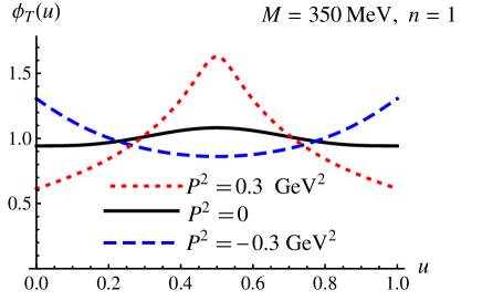
c)	d)

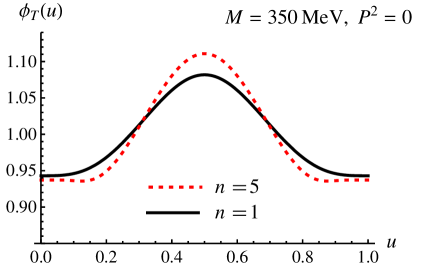
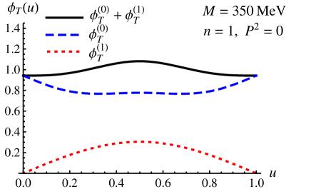
Figure 1: Leading twist tensor photon DA for: a) different photon virtualities and fixed $M=350$ MeV and $n=1$, b) different $M$ and fixed $n=1$ and $P^{2}=0$, c) different $n$ and fixed $M=350$ MeV and $P^{2}=0$, d) decomposition into contributions corresponding to local (dashed) and non-local (dotted) parts of the vector vertex for $M=350$ MeV, $n=1$ and $P^{2}=0$.

a)	b)

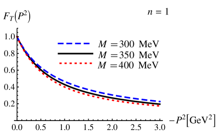
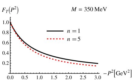
Figure 2: Tensor form factor for: a) fixed $n=1$ and different $M$, b) fixed $M=350$ MeV and two different $n=1,5$.

Tensor form factor is shown in fig. 2. It can be in principle calculated by analytical integration, which has to be performed carefully because of the complex numbers under logarithms.

V.1.2 Vector photon DA

Calculation of vector twist-2 amplitude proceeds in a similar way. After performing the traces we get

$$\psi_{V}(u)=\frac{-i4P^{+}N_{c}}{f_{3\gamma}F_{V}(P^{2})\varepsilon^{+}}{\displaystyle\int}\frac{d^{D}k}{(2\pi)^{D}}\frac{\left(T_{V}^{(0)}+T_{V}^{(1)}\right)\,\delta\left(k\cdot n-u\,n\cdot P\right)}{(k^{2}-M_{k}^{2}+i\epsilon)((k-P)^{2}-M_{k-P}^{2}+i\epsilon)}.$$ (45)

where $T_{V}^{(0)}$ and $T_{V}^{(1)}$ stand for traces corresponding to local and nonlocal parts of the photon vertex respectively:

$$T_{V}^{(0)} =\varepsilon^{+}(M_{k}M_{k-P}+\vec{k}_{\bot}^{2}-P^{2}u\bar{u})-(\vec{\varepsilon}_{\bot}\cdot\vec{k}_{\bot})P^{+}(\bar{u}+u),$$

$$T_{V}^{(1)} =-\frac{\left(M_{k}-M_{k-P}\right)\left(\bar{u}M_{k}+uM_{k-P}\right)}{k^{-}+\bar{u}\frac{P^{2}}{P^{+}}}\left[\varepsilon^{+}\left(k^{-}-u\frac{P^{2}}{P^{+}}\right)-2\,(\vec{\varepsilon}_{\bot}\cdot\vec{k}_{\bot})\right].$$ (46)

Note that single powers of $(\vec{\varepsilon}_{\bot}\cdot\vec{k}_{\bot})$ integrate to zero.

In the case of twist 2 vector DA we have to subtract the perturbative piece corresponding to $M\left(k\right)=0$. Then, the contribution to the vector photon DA coming from the local part of the vertex consists of two parts

$$\phi_{V}^{(0,a)}\left(u,P^{2}\right) =\frac{N_{c}}{4\pi^{2}f_{3\gamma}F_{V}(P^{2})}\sum_{i,j=1}^{4n+1}f_{i}f_{j}\left(\Lambda^{2}\eta_{i}^{4n}\eta_{j}^{4n}\left(\bar{u}\eta_{i}-u\eta_{j}-1\right)+M^{2}\eta_{i}^{2n}\eta_{j}^{2n}\right)$$

$$\qquad\qquad\qquad\qquad\qquad\qquad\qquad\qquad\qquad\ln\left(1+u\bar{u}p^{2}-\bar{u}\eta_{i}+u\eta_{j}\right).$$ (47)

and

$$\phi_{V}^{(0,b)}\left(u,P^{2}\right)=\frac{N_{c}}{4\pi^{2}f_{3\gamma}F_{V}(P^{2})}\left(-2u\bar{u}P^{2}\right)\sum_{i,j=1}^{4n+1}f_{i}f_{j}\eta_{i}^{4n}\eta_{j}^{4n}\ln\left(\frac{1+u\bar{u}p^{2}-\bar{u}\eta_{i}+u\eta_{j}}{u\bar{u}p^{2}}\right).$$ (48)

The addition coming from the nonlocal part of the current can be conveniently split into a sum of two contributions

$$\phi_{V}^{(1,a)}(u) =\frac{-N_{c}}{4\pi^{2}f_{3\gamma}F_{V}(P^{2})}\,M^{2}\sum_{i,j=1}^{4n+1}f_{i}f_{j}\left(\eta_{j}^{2n}-\eta_{i}^{2n}\right)\left(\bar{u}\eta_{j}^{2n}+u\eta_{i}^{2n}\right)$$

$$\qquad\qquad\qquad\qquad\qquad\qquad\qquad\qquad\qquad\ln\left(1\frac{{}}{{}}+u\bar{u}p^{2}-\bar{u}\eta_{i}+u\eta_{j}\right),$$ (49)

$$\phi_{V}^{(1,b)}(u) =\frac{N_{c}}{4\pi^{2}f_{3\gamma}F_{V}(P^{2})}(1-2u)\frac{M^{2}P^{2}}{\Lambda^{2}}\sum_{i,j=1}^{4n+1}f_{i}f_{j}\frac{\left(\eta_{i}^{2n}-\eta_{j}^{2n}\right)\left(\bar{u}\eta_{j}^{2n}+u\eta_{i}^{2n}\right)}{\left(\eta_{i}-\eta_{j}\right)}$$

$$\qquad\qquad\qquad\qquad\qquad\qquad\qquad\qquad\qquad\ln\left(1\frac{{}}{{}}+u\bar{u}p^{2}-\bar{u}\eta_{i}+u\eta_{j}\right).$$ (50)

Notice that subtraction concerns only $\phi_{V}^{\mathrm{\left(0,b\right)}}$ part since $\phi_{V}^{\mathrm{\left(1\right)}}$ is always proportional to mass.

In the tensor case the only effect due to the local vertex is a small change in the shape of the distribution. The situation is different for vector DA. When we use local current only, the vector distribution alternates in sign (recall that leading twist DAs have probabilistic interpretation). Only when we include the nonlocal part of the vertex, contributions $\phi_{V}^{(0,a)}$ and $\phi_{V}^{(1,a)}$ cancel exactly for any $P^{2}$. This is explicitly shown in fig.3.d. As a consequence $\phi_{V}$ is effectively the sum of $\phi_{V}^{(0,b)}$ and $\phi_{V}^{(1,b)}$. We plot this function in fig. 3 for different sets of model parameters.

Furthermore, since both $\phi_{V}^{(0,b)}$ and $\phi_{V}^{(1,b)}$ are explicitly proportional to $P^{2}$, normalization conditions (14) require that $F_{V}(0)=0$ as it should be in accordance with the conservation of the vector current. This condition would be violated if not for the nonlocal part of the photon vertex.

a)	b)
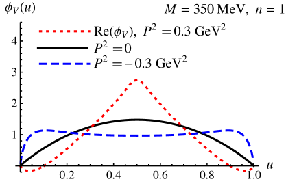
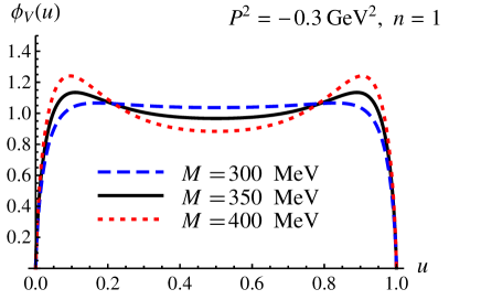
c)	d)

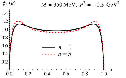
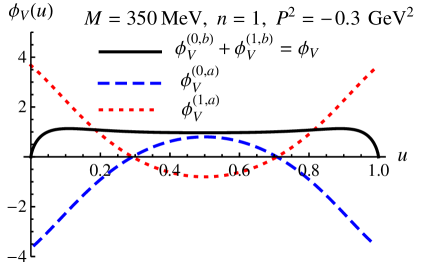
Figure 3: Leading twist vector photon DA for: a) different photon virtualities and fixed $M=350$ MeV and $n=1$, b) different $M$ and fixed $n=1$ and $P^{2}=-0.3$ GeV², c) different $n$ and fixed $M=350$ MeV and $P^{2}=-0.3$ GeV², d) decomposition into different contributions, as described in the main text; notice the exact cancelation of $\phi_{V}^{(0,a)}$ and $\phi_{V}^{(1,a)}$ following from the gauge invariance. For positive $P^{2}$ we show only real part of DA.

a)	b)

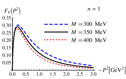
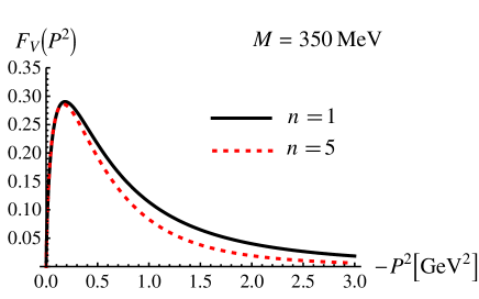
Figure 4: Vector form factor for: a) fixed $n=1$ and different $M$, b) fixed $M=350$ MeV and two different choices of $n=1,5$. Notice that the form factor vanishes for zero virtuality as required by vector current conservation.

V.2 Higher twist distributions

For higher twist distributions we encounter an additional difficulty. As shown in appendix C it turns out that they are in fact generalized functions. Due to $k^{-}=k\cdot\tilde{n}$ occurring in the numerator ($k^{+}=k\cdot n$ is fixed – see delta function in (40)), additional end point delta functions appear. They are crucial for Lorentz invariance of the integrals and in consequence for the correct normalization of the distributions. These singularities were already discussed in ref.  Dorokhov:2006qm .

V.2.1 Tensor DAs

We start with tensor DAs. For twist 3 tensor amplitude we have

$$\psi_{T}(u)=\frac{4N_{c}}{\left\langle\bar{\psi}\psi\right\rangle F_{T}(P^{2})}\frac{P^{+}}{\varepsilon^{+}}{\displaystyle\int}\frac{d^{4}k}{(2\pi)^{4}}\frac{\left(T_{T}^{(0)}+T_{T}^{(1)}\right)\,\delta\left(k\cdot n-uP^{+}\right)}{(k^{2}-M_{k}^{2}+i\epsilon)((k-P)^{2}-M_{k-P}^{2}+i\epsilon)}$$ (51)

where $T_{T}^{(0)}$ and $T_{T}^{(1)}$ stand for traces corresponding to local and nonlocal parts of the photon vertex respectively:

$$T_{T}^{(0)} =-\frac{i}{2}\varepsilon^{+}\left[P^{+}(M_{k}-M_{k-P})\left(k^{-}+\bar{u}\frac{P^{2}}{P^{+}}\right)-P^{2}(M_{k}+M_{k-P})\right],$$ (52)

$$T_{T}^{(1)} =\frac{i}{2}\frac{P^{+}\left(M_{k}-M_{k-P}\right)}{k^{-}+\bar{u}\frac{P^{2}}{P^{+}}}\left(k^{-}-u\frac{P^{2}}{P^{+}}\right)\left[\varepsilon^{+}\left(k^{-}-u\frac{P^{2}}{P^{+}}\right)-2\vec{k}_{\bot}\cdot\vec{\varepsilon}_{\bot}\right]\,.$$ (53)

Note that even powers of $\vec{k}_{\bot}\cdot\vec{\varepsilon}_{\bot}$ integrate to zero under $d^{2}\vec{k}_{\bot}$.

Luckily in the case of $\psi_{T}(u)$ contributions involving $k^{-}$ cancel out in the sum of (52) and (53) and the final result is the sum of two pieces

$$\psi_{T}^{(a)}(u) =\frac{N_{c}M}{8\pi^{2}\left\langle\bar{\psi}\psi\right\rangle\chi_{m}F_{T}(P^{2})}\left(\chi_{m}P^{2}\right)$$ (54)

$$\sum_{i,j=1}^{4n+1}f_{i}f_{j}\eta_{i}^{2n}\eta_{j}^{2n}\left[(\eta_{j}^{2n}+\eta_{i}^{2n})+2\left(1-2u\right)\left(\eta_{j}^{2n}-\eta_{i}^{2n}\right)\right]\ln\left(1\frac{{}}{{}}+u\bar{u}p^{2}-\bar{u}\eta_{i}+u\eta_{j}\right)$$

and

$$\psi_{T}^{(b)}(u) =\frac{-N_{c}M}{8\pi^{2}\left\langle\bar{\psi}\psi\right\rangle\chi_{m}F_{T}(P^{2})}\left(\chi_{m}P^{2}\right)\frac{P^{2}}{\Lambda^{2}}\left(1-2u\right)^{2}$$

$$\sum_{i,j=1}^{4n+1}f_{i}f_{j}\eta_{i}^{2n}\eta_{j}^{2n}\frac{\eta_{j}^{2n}-\eta_{i}^{2n}}{\eta_{j}-\eta_{i}}\ln\left(1\frac{{}}{{}}+u\bar{u}p^{2}-\bar{u}\eta_{i}+u\eta_{j}\right).$$ (55)

Note that $\psi_{T}$ is proportional to the same normalization constant as $\phi_{T}$ times $\left(\chi_{m}P^{2}\right)$ which means that it decouples for real photons.

In the case of twist $4$ tensor amplitude the $\delta$ function contributions do not cancel out. Performing Dirac traces we have

$$h_{T}(u)=\frac{4N_{c}P^{+\,2}}{\left\langle\bar{\psi}\psi\right\rangle\,F_{T}(P^{2})}{\displaystyle\int}\frac{d^{4}k}{(2\pi)^{4}}\frac{\left(R_{T}^{(0)}+R_{T}^{(1)}\right)\,\delta\left(k\cdot n-u\,n\cdot P\right)}{(k^{2}-M_{k}^{2}+i\epsilon)((k-P)^{2}-M_{k-P}^{2}+i\epsilon)}$$ (56)

where again the contributions of local and nonlocal parts of the vector current have been singled out:

$$R_{T}^{(0)} =-i\frac{P^{2}}{P^{+\,2}}\varepsilon^{+}(M_{k}-M_{k-P})\left(\vec{\varepsilon}_{\bot}\cdot\vec{k}_{\bot}\right)-i\left[(M_{k}-M_{k-P})k^{-}-M_{k}\frac{P^{2}}{P^{+}}\right],$$ (57)

$$R_{T}^{(1)} =\,-i\frac{P^{2}}{P^{+\,2}}\frac{M_{k}-M_{k-P}}{k^{-}+\bar{u}\frac{P^{2}}{P^{+}}}\,\left(\vec{\varepsilon}_{\bot}\cdot\vec{k}_{\bot}\right)\left[\varepsilon^{+}\left(k^{-}-u\frac{P^{2}}{P^{+}}\right)-2\left(\vec{\varepsilon}_{\bot}\cdot\vec{k}_{\bot}\right)\right]$$ (58)

Note that significant simplifications occur since single power of $\vec{k}_{\bot}\cdot\vec{\varepsilon}$ integrates to zero. Following the steps described in appendix C we finally arrive at the final formula for $h_{T}(u)$. It is convenient to split it into 4 different pieces – regular local vertex contribution:

$$h_{T}^{(0,a)}(u) =\frac{N_{c}M}{4\pi^{2}\left\langle\bar{\psi}\psi\right\rangle\chi_{m}\,F_{T}(P^{2})}\chi_{m}P^{2}{\displaystyle\sum\limits_{i,j=1}^{4n+1}}f_{i}\,f_{j}\eta_{i}^{2n}\eta_{j}^{2n}\left(u\eta_{i}^{2n}-\bar{u}\eta_{j}^{2n}\right)$$

$$\quad\quad\quad\quad\quad\quad\quad\quad\quad\quad\quad\quad\quad\ln\left(1\frac{{}}{{}}+u\bar{u}p^{2}-\bar{u}\eta_{i}+u\eta_{j}\right),$$ (59)

second local vertex contribution:

$$h_{T\text{ }}^{(0,b)}(u) =\frac{-N_{c}M}{4\pi^{2}\left\langle\bar{\psi}\psi\right\rangle\chi_{m}\,F_{T}(P^{2})}\chi_{m}\Lambda^{2}{\displaystyle\sum\limits_{i,j=1}^{4n+1}}f_{i}\,f_{j}\,\eta_{i}^{2n}\eta_{j}^{2n}\left(\eta_{j}^{2n}-\eta_{i}^{2n}\right)\left(\left(\eta_{i}-\eta_{j}\right)+\frac{{}}{{}}(1-2u)p^{2}\right)$$

$$\quad\quad\quad\quad\quad\quad\quad\quad\quad\quad\quad\quad\quad\quad\quad\quad\quad\quad\ln\left(1\frac{{}}{{}}+u\bar{u}p^{2}-\bar{u}\eta_{i}+u\eta_{j}\right)$$ (60)

that integrates to zero with $\delta$-function contribution

$$h_{T\text{ }}^{(0,\mathrm{delta})}(u) =\frac{N_{c}M}{4\pi^{2}\left\langle\bar{\psi}\psi\right\rangle\chi_{m}\,F_{T}(P^{2})}\chi_{m}\Lambda^{2}{\displaystyle\sum\limits_{i,j=1}^{4n+1}}f_{i}\,f_{j}\,\eta_{i}^{2n}\eta_{j}^{2n}\left(\eta_{i}^{2n}-\eta_{j}^{2n}\right)$$

$$\left[(1+\eta_{j})\ln\left(1+\eta_{j}\right)\delta(u-1)\frac{{}}{{}}-(1+\eta_{i})\ln\left(1+\eta_{i}\right)\delta(u)\right]$$ (61)

and hence does not contribute to the normalization, and the contribution corresponding to the nonlocal part of the photon vertex:

$$h_{T}^{(1)}(u) =\frac{N_{c}M}{4\pi^{2}\left\langle\bar{\psi}\psi\right\rangle\,\chi_{m}F_{T}(P^{2})}\chi_{m}P^{2}\,\sum_{i,j=1}^{4n+1}f_{i}f_{j}\eta_{i}^{2n}\eta_{j}^{2n}\left(1\frac{{}}{{}}+u\bar{u}p^{2}-\bar{u}\eta_{i}+u\eta_{j}\right)$$

$$\qquad\qquad\qquad\qquad\qquad\qquad\qquad\frac{\eta_{i}^{2n}-\eta_{j}^{2n}}{\eta_{i}-\eta_{j}}\ln\left(1\frac{{}}{{}}+u\bar{u}p^{2}-\bar{u}\eta_{i}+u\eta_{j}\right).$$ (62)

The delta contribution $h_{T}^{(0,\mathrm{delta})}$ can be rewritten using the expression (39) for $f_{3\gamma}$ and the identities given in Appendix A:

$$h_{T}^{(0,\mathrm{delta})}(u) =\frac{-1}{F_{T}(P^{2})}\left[\delta(u-1)+\delta(u)\right]$$ (63)

Note that the fact that the sum of (60) and (61) integrates over $du$ to zero is a consequence of Lorentz invariance discussed in sect. IV (see eq. (23)). Therefore only $h_{T}^{(0,a)}$ and $h_{T}^{(1)}(u)$ contribute to the normalization condition (13) given by $(\chi_{m}P^{2})$. If not for the $\delta$-term $h_{T}^{(0,b)}$ would also contribute to the norm spoiling the normalization condition.

Full results (with nonlocal current) for twist 3 $\psi_{T}$ and twist 4 $h_{T}$ tensor distributions are show in figs. 5 and 6 respectively.

a)	b)
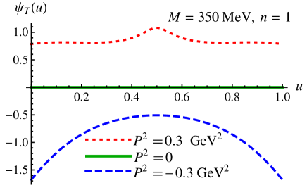
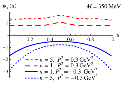
c)	d)

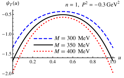
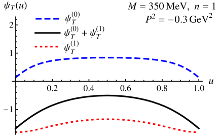
Figure 5: Tensor twist 3 photon DA for: a) different photon virtualities and fixed $M=350$ MeV and $n=1$ (for $P^{2}=0$ it is identically zero), b) different $n$ and $P^{2}$ for fixed $M=350$ MeV, c) different $M$ and fixed $n=1$ and $P^{2}=-0.3$ GeV², d) decomposition into contributions corresponding to local (dashed) and non-local (dotted) parts of the vector vertex.

a)	b)
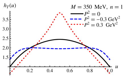
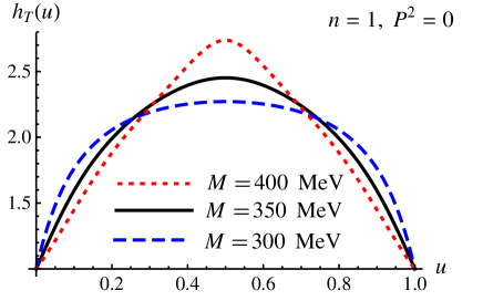
c)	d)

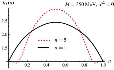
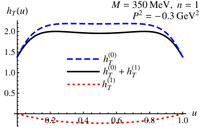
Figure 6: Tensor twist 4 photon DA (without end point delta functions) for: a) different photon virtualities and fixed $M=350$ MeV and $n=1$, b) various $M$ and fixed $n=1$ and $P^{2}=0$, c) two choices of $n=1,5$ and fixed $M=350$ MeV and $P^{2}=0$, d) decomposition into contributions corresponding to local (dashed) and non-local (dotted) parts of the vector vertex.

V.2.2 Vector DAs

In the case of higher twist vector DAs, $\psi_{V}$ and $h_{V}$, calculations are basically the same, with the restriction that we have to perform subtractions similarly to the twist 2 case. For twist 3 amplitude we obtain:

$$\psi_{V}(u)=\frac{i4N_{c}P^{+}}{f_{3\gamma}F_{V}(P^{2})}{\displaystyle\int}\frac{d^{4}k}{(2\pi)^{4}}\frac{\left(T_{V}^{(0)}+T_{V}^{(1)}\right)\,\delta\left(k\cdot n-u\,n\cdot P\right)}{(k^{2}-M_{k}^{2})((k-P)^{2}-M_{k-P}^{2})}$$ (64)

with

$$T_{V}^{(0)} =\left[2(\vec{\varepsilon}_{\bot}\cdot\vec{k}_{\bot})^{2}-\vec{k}_{\bot}^{\,2}\right]-\varepsilon^{+}(\vec{\varepsilon}_{\bot}\cdot\vec{k}_{\bot})\left(k^{-}-u\frac{P^{2}}{P^{+}}\right)$$

$$-\frac{1}{2}(1-2u)P^{+}k^{-}-\frac{1}{2}uP^{2}-M_{k}M_{k-P}.$$ (65)

In fact after integrating over the transverse angle the terms in the first line vanish. Next

$$T_{V}^{(1)}=\frac{(\vec{\varepsilon}_{\bot}\cdot\vec{k}_{\bot})}{P^{+}}\frac{\left(M_{k}^{2}-M_{k-P}^{2}\right)}{k^{-}+\bar{u}\frac{P^{2}}{P^{+}}}\left[\varepsilon^{+}\left(k^{-}-u\frac{P^{2}}{P^{+}}\right)-2(\vec{k}_{\bot}\cdot\vec{\varepsilon}_{\bot})\right].$$ (66)

Again only quadratic term $(\vec{\varepsilon}_{\bot}\cdot\vec{k}_{\bot})^{2}$ survives integration over the transverse angle. The result can be split into a regular part coming from the local part of the vertex:

$$\psi_{V}^{(0,\,\text{reg})}(u) =\frac{N_{c}}{8\pi^{2}f_{3\gamma}F_{V}(P^{2})}{\displaystyle\sum\limits_{i,j=1}^{4n+1}}f_{i}\,f_{j}\,\eta_{i}^{2n}\eta_{j}^{2n}\ln\left(\frac{1+u\bar{u}p^{2}-\bar{u}\eta_{i}+u\eta_{j}}{u\bar{u}p^{2}}\right)$$

$$\left(\left(1+2u\bar{u}\right)\eta_{i}^{2n}\eta_{j}^{2n}P^{2}+2M^{2}+\frac{{}}{{}}(1-2u)(\eta_{i}-\eta_{j})\eta_{i}^{2n}\eta_{j}^{2n}\Lambda^{2}\right),$$ (67)

the part with delta functions also coming from the local part of the vertex:

$$\psi_{V}^{(0,\,\text{delta})}(u)=\frac{-N_{c}}{8\pi^{2}f_{3\gamma}F_{V}(P^{2})}\Lambda^{2}{\displaystyle\sum\limits_{i=1}^{4n+1}}f_{i}\,\eta_{i}^{4n}(1+\eta_{i})\ln\left(1+\eta_{i}\right)\left[\delta(u-1)\frac{{}}{{}}+\delta(u)\right]$$ (68)

and the nonlocal part:

$$\psi_{V}^{(1)}(u) =\frac{N_{c}}{8\pi^{2}f_{3\gamma}F_{V}(P^{2})}2M^{2}\,\sum_{i,j=1}^{4n+1}f_{i}f_{j}(\eta_{j}^{2n}\,+\eta_{i}^{2n})\left(1-\eta_{i}\bar{u}+\eta_{j}u+u\bar{u}r^{2}\right)$$

$$\qquad\qquad\qquad\frac{\eta_{i}^{2n}-\eta_{j}^{2n}}{\eta_{i}-\eta_{j}}\;\ln\left(1+u\bar{u}p^{2}-\bar{u}\eta_{i}+u\eta_{j}\right)$$ (69)

The part with delta functions can be rewritten as

$$\psi_{V}^{(0,\,\text{delta})}(u)=\frac{-1}{2F_{V}(P^{2})}\left[\delta(u-1)+\delta(u)\right],$$ (70)

where we used (39) and the identity $\Lambda^{2}\eta_{i}^{4n}(1+\eta_{i})=M^{2}$ following from equation (27) for zeros of $G(z)$.

Next we calculate twist 4 vector distribution amplitude $h_{V}(u)$:

$$h_{V}(u)=\frac{i4N_{c}P^{+}}{f_{3\gamma}F_{V}(P^{2})}\,\frac{\left(P^{+}\right)}{2P^{2}}{\displaystyle\int}\frac{d^{4}k}{(2\pi)^{4}}\frac{\left(R_{V}^{(0)}+R_{V}^{(1)}\right)\,\delta\left(k\cdot n-u\,n\cdot P\right)}{(k^{2}-M_{k}^{2})((k-P)^{2}-M_{k-P}^{2})}$$ (71)

where the traces read

$$R_{V}^{(0)} =\left(k^{-}\right)^{2}-\frac{P^{2}}{P^{+}}k^{-}-\frac{P^{2}}{\left(P^{+}\right)^{2}}k_{T}^{2}-M_{k}M_{k-P}$$ (72)

$$R_{V}^{(1)} =\frac{k^{-}-\frac{P^{2}}{P^{+}}u}{k^{-}+\bar{u}\frac{P^{2}}{P^{+}}}\,\left[k^{-}\left(M^{2}_{k}-M^{2}_{k-P}\right)-M_{k}\left(M_{k}-M_{k-P}\right)\right]$$ (73)

The only additional complication is due to the second derivative of delta function – the details can be found appendix C eqs.(114)–(116). Results for the local part read:

$$h_{V}^{(0,\,\text{reg})}(u) =\frac{-N_{c}}{8\pi^{2}f_{3\gamma}F_{V}(P^{2})}\,2{\displaystyle\sum\limits_{i,j=1}^{4n+1}}f_{i}\,f_{j}\,\eta_{i}^{2n}\eta_{j}^{2n}\ln\left(\frac{1+u\bar{u}p^{2}-\bar{u}\eta_{i}+u\eta_{j}}{u\bar{u}p^{2}}\right)$$

$$\bigg{(}2u\bar{u}\,\eta_{i}^{2n}\eta_{j}^{2n}P^{2}-2M^{2}+\eta_{i}^{2n}\eta_{j}^{2n}\left(2\eta_{i}-\eta_{j}+1-3u(\eta_{i}-\eta_{j})\right)\Lambda^{2}$$ (74)

$$+\frac{(\eta_{i}-\eta_{j})^{2}\Lambda^{4}}{P^{2}}\bigg{)},$$ (75)

and

$$h_{V}^{(0,\,\text{delta})}(u) =\frac{-N_{c}}{8\pi^{2}f_{3\gamma}F_{V}(P^{2})}\,\frac{2\,\Lambda^{2}}{P^{2}}\bigg{\{}-2M^{2}{\displaystyle\sum\limits_{i=1}^{4n+1}}f_{i}\,\ln\left(1+\eta_{i}\right)$$

$$\qquad\qquad\qquad\qquad\left[(1+\eta_{i})\,\left[\delta(u)+\delta(u-1)\right]+p^{2}\delta(u)\right]$$

$$+\Lambda^{2}\,{\displaystyle\sum\limits_{i,j=1}^{4n+1}}f_{i}\,f_{j}\eta_{i}^{4n}\eta_{j}^{4n}\frac{1}{2}\ln\left(\frac{1+u\bar{u}p^{2}-\bar{u}\eta_{i}+u\eta_{j}}{u\bar{u}p^{2}}\right)\left(1+u\bar{u}p^{2}-\bar{u}\eta_{i}+u\eta_{j}\right)^{2}$$

$$\qquad\qquad\qquad\qquad\left[\delta^{\prime}(u)+\delta^{\prime}(u-1)\right]\bigg{\}},$$ (76)

and for the contribution coming from the nonlocal part of the photon vertex:

$$h_{V}^{(1,\,\text{reg})}(u) =\frac{-N_{c}}{8\pi^{2}f_{3\gamma}F_{V}(P^{2})}\,\frac{2M^{2}\,\Lambda^{2}}{P^{2}}{\displaystyle\sum\limits_{i,j=1}^{4n+1}}f_{i}\,f_{j}\,\ln\left(1+u\bar{u}p^{2}-\bar{u}\eta_{i}+u\eta_{j}\right)$$

$$\qquad\qquad\qquad\frac{\eta_{i}^{2n}-\eta_{j}^{2n}}{\eta_{i}-\eta_{j}}\,\left(\eta_{i}-\eta_{j}-(2u-1)p^{2}\right)\,\left(\left(\eta_{i}^{2n}+\eta_{j}^{2n}\right)-p^{2}\,\eta_{j}^{2n}\right),$$ (77)

$$h_{V}^{(1,\,\text{delta})}(u) =\frac{-N_{c}}{8\pi^{2}f_{3\gamma}F_{V}(P^{2})}\,\frac{2M^{2}\,\Lambda^{2}}{P^{2}}{\displaystyle\sum\limits_{i=1}^{4n+1}}f_{i}\,(1+\eta_{i})\ln\left(1+\eta_{i}\right)\,\left[\delta(u)+\delta(u-1)\right].$$ (78)

We note that

$$\int_{0}^{1}\,h_{V}^{(0,\,\text{delta})}(u)\,du=\frac{-N_{c}}{8\pi^{2}f_{3\gamma}F_{V}(P^{2})}\,\frac{-4\,M^{2}\,\Lambda^{2}}{P^{2}}{\displaystyle\sum\limits_{i=1}^{4n+1}}f_{i}\,(1+\eta_{i})\ln\left(1+\eta_{i}\right),$$ (79)

thus it cancels with $\int_{0}^{1}\,h_{V}^{(1,\,\text{ delta})}(u)\,du$ as can be easily seen.

Our results are shown in figs. 7 and 8 for twist 3 and twist 4 respectively. The magnitude of both distributions is growing unlimitedly when photon becomes softer (obviously distributions multiplied by the vector form factor remain finite). Notice however that for the real photon $h_{V}$ decouples.

a)	b)
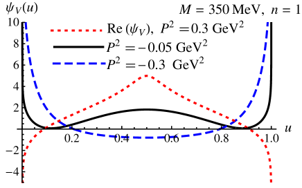
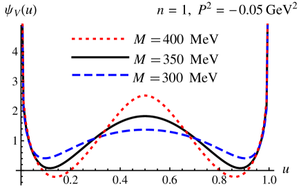
c)	d)

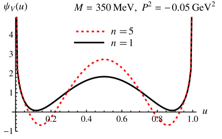
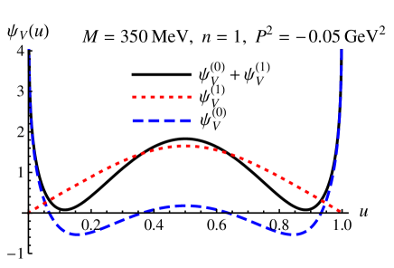
Figure 7: Vector twist 3 photon DA for: a) different photon virtualities and fixed $M=350$ MeV and $n=1$, b) various $M$ and fixed $n=1$ and $P^{2}=-0.05$ GeV², c) two choices of $n=1,5$ and fixed $M=350$ MeV and $P^{2}=-0.05$ GeV², d) decomposition into contributions corresponding to local (dashed) and non-local (dotted) parts of the vector vertex.

a)	b)
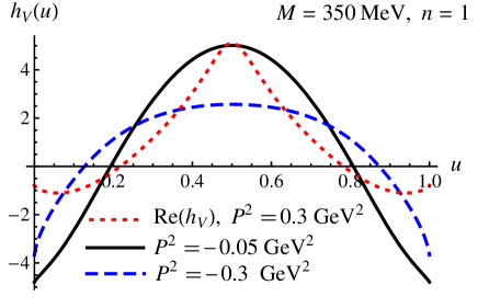
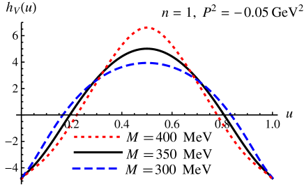
c)	d)

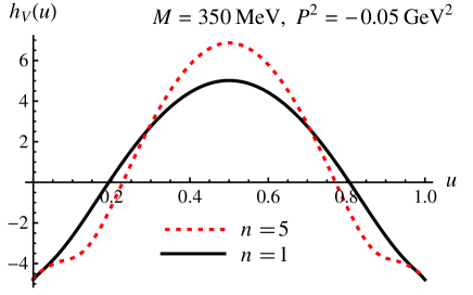
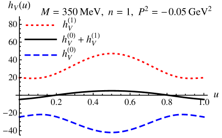
Figure 8: Vector twist 4 photon DA for: a) different photon virtualities and fixed $M=350$ MeV and $n=1$, b) various $M$ and fixed $n=1$ and $P^{2}=-0.05$ GeV²,, c) two choices of $n=1,5$ and fixed $M=350$ MeV and $P^{2}=-0.05$ GeV², d) decomposition into contributions corresponding to local (dashed) and non-local (dotted) parts of the vector vertex.

V.2.3 Axial DA

We have only one distribution in the axial vector channel which is of twist 3. When inverting the definition (9), due to presence of $\lambda$ on the right hand side, we obtain the expression for the derivative of DA rather then for DA itself

$$\tilde{\psi}_{A}^{\prime}\left(u\right) =\psi_{A}^{\prime}\left(u\right)+\psi_{A}\left(0\right)\delta\left(u\right)-\psi_{A}\left(1\right)\delta\left(\bar{u}\right)$$ (80)

$$=-i\frac{8N_{c}}{f_{3\gamma}\,F_{A}(P^{2})}\int\frac{d^{D}k}{\left(2\pi\right)^{D}}\frac{T_{A}^{(0)}}{(k^{2}-M_{k}^{2})((k-P)^{2}-M_{k-P}^{2})}\delta\left(k\cdot n-uP^{+}\right),$$

with

$$T_{A}^{(0)}=-\frac{P^{+2}}{2}\left(k^{-}-\frac{P^{2}}{P^{+}}u\right)-\varepsilon^{+}P^{2}\,(\vec{\varepsilon}_{\bot}\cdot\vec{k}_{\bot}).$$ (81)

In the case of axial DA the nonlocal part of the vertex does not give any contribution. This is simply because the Dirac trace is equal to zero. To obtain $\psi_{A}\left(u\right)$ one has to integrate (80) over $du^{\prime}$ from $0$ to $u$:

$$\psi_{A}\left(u\right)={\displaystyle\int\limits_{0}^{u}}\tilde{\psi}_{A}^{\prime}\left(u^{\prime}\right)du^{\prime}.$$ (82)

Notice that the end point contributions cancel out and one might get an impression that $\psi_{A}\left(u\right)$ is determined up to a constant. Fortunately we have at our disposal an independent formula for $F_{A}(P^{2})$ given by eq. (12) (see also eq. (126) in appendix D) and the normalization condition (15) that fix the value of $\psi_{A}(0)=\psi_{A}(1)\neq 0$ at nonzero value.

As in the case of vector twist 2 DA $\psi_{A}(u)$ is UV divergent and requires subtraction of the perturbative part. The result splits into a regular part

$$\,\tilde{\psi}_{A}^{(a)\,\prime}(u) =\frac{N_{c}}{4\pi^{2}f_{3\gamma}\,F_{A}(P^{2})}{\displaystyle\sum\limits_{i,j=1}^{4n+1}}f_{i}\,f_{j}\,\eta_{i}^{4n}\eta_{j}^{4n}\left(\left(\eta_{i}-\eta_{j}\right)\Lambda^{2}+(1-2u)P^{2}\right)$$ (83)

$$\,\,\,\qquad\qquad\,\,\,\qquad\qquad\,\,\,\qquad\ln\left(\frac{1+u\bar{u}p^{2}-\bar{u}\eta_{i}+u\eta_{j}}{u\bar{u}p^{2}}\right)$$

and the piece involving $\delta$ functions:

$$\,\tilde{\psi}_{A}^{(a)\,\prime}(u)=\frac{N_{c}}{4\pi^{2}f_{3\gamma}\,F_{A}(P^{2})}\Lambda^{2}{\displaystyle\sum\limits_{i=1}^{4n+1}}f_{i}\,\eta_{i}^{4n}\,(1+\eta_{i})\ln\left(1+\eta_{i}\right)\left[\delta(u)\frac{{}}{{}}-\delta(u-1)\right].$$ (84)

Note that $\eta_{i}^{4n}\,(1+\eta_{i})=r^{2}$, and in virtue of (39)

$$\,\tilde{\psi}_{A}^{(a)\,\prime}(u)=\frac{1}{\,F_{A}(P^{2})}\left[\delta(u)\frac{{}}{{}}-\delta(u-1)\right].$$ (85)

The form factor $F_{A}(P^{2})$ and $\psi_{A}(u)$ itself is shown in fig. 9. We obtain the following values for axial form factor at zero momenta: $F_{A}\left(0\right)\approx 0.77$ for $M=350\,\mathrm{MeV}$, $F_{A}\left(0\right)\approx 0.79$ for $M=300\,\mathrm{MeV}$ and $F_{A}\left(0\right)\approx 0.75$ for $M=400\,\mathrm{MeV}$.

a)	b)
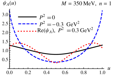
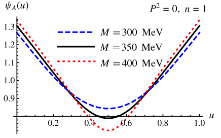
c)	d)

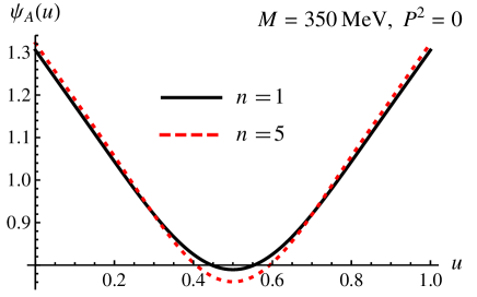
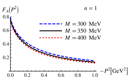
Figure 9: Axial photon DA for: a) different photon virtualities and fixed $M=350$ MeV and $n=1$, b) various $M$ and fixed $n=1$ and $P^{2}=0$, c) two choices of $n=1,5$ and fixed $M=350$ MeV and $P^{2}=0$. d) Axial form factor for different choices of $M$ (there is almost no $n$ dependence).

VI Summary

In this work we calculated analytically a set of photon distribution amplitudes up to twist four in tensor, vector and axial vector channels. We used nonlocal chiral quark model with momentum dependent quark mass. In order to get a correct behavior of low energy matrix elements we modified vector vertices (making them nonlocal) in such a way that Ward-Takahashi identities were fulfilled (1). Similar, although numerical calculation was already done in ref. Dorokhov:2006qm . They also used instanton motivated nonlocal model with dressed vertices, taking into account rescattering in the $\rho$ meson channel. The shape of the mass dependence on momentum was chosen as an exponent decreasing with $k^{2}$. Here we use $F\left(k\right)$ as given by (17) and neglect rescattering which turns out to be small.

First we obtained numerical estimates for quark condensate $\left\langle\bar{\psi}\psi\right\rangle$, magnetic susceptibility $\chi_{m}$ and decay constant $f_{3\gamma}$ in our model. For larger values of constituent quark mass $M$ or power $n$ our results are getting close to the ones of ref. Dorokhov:2006qm . Unlike $\left\langle\bar{\psi}\psi\right\rangle$ and $\chi_{m}$ the value of $f_{3\gamma}$ is rather stable as far as model parameters are concerned. Using evolution equations (following refs. Ball:2002ps ; Dorokhov:2006qm ) we find that for $M=350\,\mathrm{MeV}$ and $n=5$, the scale of our model is about $\mu\approx 500\,\mathrm{MeV}$ (this estimation was done using $\left\langle\bar{\psi}\psi\right\rangle$, $\chi_{m}$, $f_{3\gamma}$ as given by sum rules at $1\,\mathrm{GeV}$ scale and evolving them backwards down to the model values). This is in rough agreement with the scale of the instanton liquid model which is believed to be of the order of 600 MeV Diakonov:1983hh .

Next let us discuss the properties of the distribution amplitudes obtained within the present approach. Leading twist amplitudes are not very sensitive to the value of power $n$. However it seems that higher twist DAs are rather strongly model dependent.

Comparing our results with those of ref. Dorokhov:2006qm we find some similarities, but also some discrepancies. Tensor leading twist DAs are in fact the same. For real photons they are almost constant with small maximum at $u=1/2$ and they do not vanish at the end points. The contribution of the nonlocal part of the vertex is rather small, it is however producing the small maximum in the middle. For $P^{2}\neq 0$ the end points move up for negative $P^{2}$ and down for positive $P^{2},$ whereas the middle value behaves in the opposite way.

Twist 2 vector DA ($\phi_{V}$) should decouple for $P^{2}=0$. Here the importance of gauge invariance shows up. We find cancelation of two contributions to $\phi_{V}$ coming from the local and nonlocal parts of the photon vertex which are not proportional to $P^{2}$. The remaining part is therefore proportional to $P^{2}$ and decouples as required by the gauge invariance. We find that $\phi_{V}$ vanishes at the end points and develops minimum in the middle for $P^{2}\ll 0$, whereas for $P^{2}\gg 0$ it has a bell-like shape with a small dip in the middle. This behavior is very different from the one obtained in ref. Dorokhov:2006qm where $\phi_{V}$ is almost flat and does not vanish at the end points. However both vector and also tensor form factors are quite similar in both cases.

One has to note that because of the subtraction of the perturbative part that is required in this case, $\phi_{V}$ develops imaginary part for positive photon virtualities, so in this case we only discuss the real part.

As far as higher twist DAs are concerned the situation is as follows.

Our tensor twist 3 DA ($\psi_{T}$) is identically zero for $P^{2}=0$, because it is simply proportional to $P^{2}$. For $P^{2}<0$ it is negative and has the shape of inverted "U", similarly to the one of ref. Dorokhov:2006qm . In this case DA is a regular function without $\delta$-type singularities. Vector twist 3 DA ($\psi_{V}$) in our case blows up at the end points; such behavior is not seen in ref. Dorokhov:2006qm . However, similarly to ref. Dorokhov:2006qm we also obtained delta-type singularities at the edges of the physical support. Twist 3 axial DAs ($\psi_{A}$) in both cases show similar behavior: they do not vanish at the end points and have a minimum for $u=1/2$. Despite the fact that for $P^{2}=0$ axial vector DAs both in our case and in the case of ref. Dorokhov:2006qm look similar, the axial form factors behave differently for $P^{2}<0$. In our case $F_{A}(P^{2})$ vanishes at large negative momenta in contrary to the one of ref. Dorokhov:2006qm that tends to unity in the same limit.

Regular part (without delta-type singularities) of twist 4 tensor DA ($h_{T}$) is in our case positive and vanishes at the end points for $P^{2}=0$ whereas in ref. Dorokhov:2006qm it is negative and does not vanish at the end points. For space-like photon momentum $P^{2}<0$ we see some similarity in shape between our $h_{T}$ and $-h_{T}$ of ref. Dorokhov:2006qm . Vector twist 4 DA ($h_{V}$) is in our case a result of large cancelation of the positive non-local piece and the negative local piece. Its properties are not discussed in detail in ref. Dorokhov:2006qm .

The only phenomenologically accessible photon distribution amplitude is the leading twist tensor DA – $\phi_{T}$. It is almost flat and does not vanish at the end points. This behavior is seen in our model and in other models discussed in ref. Dorokhov:2006qm and also in refs. Praszalowicz:2001wy ; Petrov:1998kg . Flat DA is characteristic for the elementary point-like particle, however, it is violating factorization theorems of QCD that require the DAs to vanish for $u=0,1$. Formal evolution of such an amplitude is questionable, not only because the Gegenbauer series is not convergent at the end points, but also, because potentially large contributions coming from the vicinity of $u=0,1$ are not summed by the ERBL evolution equations Radyushkin .

Appendix A Identities

In this appendix we summarize some of the identities used in this paper that deal with the sums of factors $f_{i}$ and powers of $\eta_{i}$. Some of them have been already introduced in ref. Praszalowicz:2001wy , but the general proofs have not been given. For definiteness let us recall that $\eta_{i},$ $i=1,\ldots,4n+1$ are the solutions of the algebraic equation $G\left(z\right)=z^{4n+1}+z^{4n}-r^{2}=0$. We denote

$$f_{i}=\prod_{j\neq i}\left(\eta_{i}-\eta_{j}\right)^{-1}.$$

For any set of $4n+1$ complex numbers $\eta_{i}$ (not necessarily satisfying $G\left(z\right)=0$) we have

$$\sum_{i=1}^{4n+1}f_{i}\eta_{i}^{N}=\begin{cases}1&\mathrm{for}\,N=4n,\\ 0&\mathrm{for\,}N<4n.\end{cases}$$ (86)

To prove (86) let’s define the following function

$$f\left(z\right)=\frac{z^{M}}{\prod_{i=1}^{4n+1}\left(z-\eta_{i}\right)},$$ (87)

where $M\leq 4n$ and integrate it over a circle with infinite radius. On one hand we can use residue technique to get the sum entering (86), on the other hand, direct integration over the large circle gives right hand side of (86).

If, in addition, $\eta_{i}$ satisfies $G\left(\eta_{i}\right)=0$ then

$$\sum_{i=1}^{4n+1}f_{i}\eta_{i}^{P}=\left(-1\right)^{P}$$ (88)

for $4n\leq P\leq 8n$. This can be proven in the following way. Notice that for $P=4n$ equality (88) is satisfied due to (86). Let us move to $P=4n+1$, that is we want to calculate

$$x=\sum_{i=1}^{4n+1}f_{i}\eta_{i}^{4n+1}.$$ (89)

Adding to this equation the result for $P=4n$ we get

$$\sum_{i=1}^{4n+1}f_{i}\left(\eta_{i}^{4n+1}+\eta_{i}^{4n}\right)=x+1.$$ (90)

Using the fact that $G\left(\eta_{i}\right)=\eta_{i}^{4n+1}+\eta_{i}^{4n}-r^{2}=0$ and (86) we have

$$x+1=r^{2}\sum_{i=1}^{4n+1}f_{i}=0.$$ (91)

and $x=-1$. This procedure can be repeated several times to prove (88) until $P=8n$.

For any set of $4n+1$ complex numbers $\eta_{i}$ we have the following identity

$$\sum_{i=1}^{4n+1}f_{i}\eta_{i}^{4n+1}=\sum_{i=1}^{4n+1}\eta_{i}.$$ (92)

Imposing in addition the constraint $G\left(\eta_{i}\right)=0$ we get $\sum_{i}^{4n+1}\eta_{i}=-1.$ The proof is similar to the one of (86), however we integrate the following function

$$g\left(z\right)=\frac{z^{4n+1}}{\left(z-\eta_{1}\right)\left(z-\eta_{2}\right)\ldots\left(z-\eta_{i}\right)^{2}\ldots\left(z-\eta_{4n+1}\right)}.$$ (93)

After several algebraic steps we arrive at (92).

Appendix B Pion decay constant

In our model Birse-Bowler formula (18) for pion decay constant reduces to the following form

$$F_{\pi}^{2}=-\frac{N_{c}M^{2}}{4\pi^{2}}\sum_{i,j=1}^{4n+1}f_{i}f_{j}\eta_{i}^{2n}\big{(}\left(1+2n\left(1+2n\right)\right)\eta_{j}^{2n+1}+\left(1+4n\left(1+3n\right)\right)\eta_{j}^{2n}\\ +2n\left(1+6n\right)\eta_{j}^{2n-1}+4n^{2}\eta_{j}^{2n-2}\big{)}\bigg{(}\frac{\epsilon_{ij}}{\eta_{i}-\eta_{j}}\left(\ln\left(1+\eta_{i}\right)-\ln\left(1+\eta_{j}\right)\right)+\frac{\delta_{ij}}{1+\eta_{i}}\bigg{)}$$ (94)

where $\epsilon_{ij}$ is $0$ for $i=j$ and $1$ otherwise, while $\delta_{ij}$ is Kronecker delta.

Appendix C Light-cone integrals in Schwinger representation

Here we summarize formulae used to perform $d^{D}k$ loop integration in the presence of $\delta(n\cdot\kappa-u\,n\cdot p)$. We will consider three cases when the numerator contains no $k^{-}$ at all and one or two powers of $k^{-}$. We follow closely the method of ref. BroniowskiTDA .

Consider loop integral (26) and apply to it (28):

$$\mathcal{J}=\mathcal{A}\Lambda^{D-5}\int\frac{d^{D}\kappa}{\left(2\pi\right)^{D}}\delta(n\cdot\kappa-u\,n\cdot p){\displaystyle\sum\limits_{i,j=1}^{4n+1}}f_{i}f_{j}\frac{\eta_{i}^{4n}\eta_{j}^{4n}\mathcal{N}}{(z_{1}-\eta_{i})(z_{2}-\eta_{j})}$$ (95)

expressed in terms of scaled variables (24). Here $\mathcal{N}$ is the numerator to be specified later. Recall that

$$z_{1}=\left(\kappa-p\right)^{2}-1+i\epsilon,\;z_{2}=\kappa^{2}-1+i\epsilon.$$ (96)

We shall now make continuation to the Euclidean metric:

$$\kappa^{0}=i\kappa^{4}$$ (97)

with

$$\kappa^{2}\rightarrow-\vec{\kappa}^{2},\;\;\kappa\cdot p\rightarrow-\vec{\kappa}\cdot\vec{p},\;\;n\cdot\kappa\rightarrow-\vec{n}\cdot\vec{\kappa}$$ (98)

where arrows denote $D$ dimensional Euclidean vectors. Therefore

$$\mathcal{J}=i\mathcal{A}\Lambda^{D-5}\int\frac{d^{D}\vec{\kappa}}{\left(2\pi\right)^{D}}\delta(\vec{n}\cdot\vec{\kappa}+up^{+}){\displaystyle\sum\limits_{i,j=1}^{4n+1}}f_{i}f_{j}\frac{\eta_{i}^{4n}\eta_{j}^{4n}\mathcal{N}}{(\vec{\kappa}^{2}+1+\eta_{i})((\vec{\kappa}-\vec{p})^{2}+1+\eta_{j})}.$$ (99)

We shall parametrize now

$$\frac{1}{(\vec{\kappa}^{2}+1+\eta_{i})((\vec{\kappa}-\vec{p})^{2}+1+\eta_{j})}={\displaystyle\int\limits_{0}^{\infty}}d\alpha{\displaystyle\int\limits_{0}^{\infty}}d\beta\,e^{-\alpha(\vec{\kappa}^{2}+1+\eta_{i})-\beta((\vec{\kappa}-\vec{p})^{2}+1+\eta_{j})}$$ (100)

and

$$\delta(\vec{n}\cdot\vec{\kappa}+up^{+})={\displaystyle\int\limits_{-\infty}^{\infty}}\frac{d\lambda}{2\pi}e^{-i\lambda(\vec{n}\cdot\vec{\kappa}+up^{+})}.$$ (101)

It is convenient to introduce new variables:

$$\alpha+\beta=s,\;\beta=ys,\;\alpha=(1-y)s=-\bar{y}s.$$ (102)

Integration measure reads then

$${\displaystyle\int\limits_{0}^{\infty}}d\alpha{\displaystyle\int\limits_{0}^{\infty}}d\beta={\displaystyle\int\limits_{0}^{\infty}}s\,ds{\displaystyle\int\limits_{0}^{1}}dy.$$ (103)

Finally we will shift momentum

$$\vec{\kappa}=\vec{\kappa}^{\,\prime}+\left(y\,\vec{p}-i\frac{\lambda}{2s}\,\vec{n}\right).$$ (104)

In these new variables we have

$$\mathcal{J} =i\mathcal{A}\Lambda^{D-5}{\displaystyle\sum\limits_{i,j=1}^{4n+1}}f_{i}\,f_{j}\,\eta_{i}^{4n}\eta_{j}^{4n}{\displaystyle\int\limits_{0}^{1}}dy\int\frac{d\lambda}{2\pi}e^{-i\lambda p^{+}(u-y)}$$

$${\displaystyle\int\limits_{0}^{\infty}}s\,dse^{-s\left[1-\bar{y}\eta_{i}+y\eta_{j}+y\bar{y}\,p^{2}\right]}\int\frac{d^{D}\vec{\kappa}^{\,\prime}}{\left(2\pi\right)^{D}}\mathcal{N}e^{-s\vec{\kappa}^{\,\prime\,2}}.$$ (105)

Further calculations depend on the nature of $\mathcal{N}$. If $\mathcal{N}$ can be expressed entirely in terms of $z_{1,2}$ then, in virtue of (28), it is enough to replace pertinent powers of $z_{1,2}^{N}\rightarrow\eta_{i,j}^{N}$ and perform Gaussian integration over $\kappa^{\prime}$. Let us denote such an integral as $\mathcal{J}_{0}$. Also integral over $d\lambda$ is trivial. In the following we shall need also integrals with $\lambda$ and $\lambda^{2}$ which read:

$$\int\frac{d\lambda}{2\pi}\{1,\lambda,\lambda^{2}\}e^{-i\lambda p^{+}(u-y)}=\frac{1}{p^{+}}\left\{1,-\frac{i}{p^{+}}\partial_{y},-\frac{1}{p^{+\,2}}\partial_{y}^{2}\right\}\delta(u-y).$$ (106)

Hence (for $D=4-2\varepsilon$) we get

$$\mathcal{J}_{0}=i\mathcal{A}\left(\frac{1}{4\pi}\right)^{2-\varepsilon}\frac{\Lambda^{-1-2\varepsilon}}{p^{+}}{\displaystyle\sum\limits_{i,j=1}^{4n+1}}f_{i}\eta_{i}^{4n}\,f_{j}\eta_{j}^{4n}\mathcal{N}(\eta_{i},\eta_{j}){\displaystyle\int\limits_{0}^{\infty}}\,dss^{\varepsilon-1}e^{-s\left[1-\bar{u}\eta_{i}+u\eta_{j}+u\bar{u}\,p^{2}\right]}.$$ (107)

In order to perform the integral over $ds$ we shall use

$${\displaystyle\int\limits_{0}^{\infty}}\,dss^{\varepsilon-1-n}e^{-s\left[\cdots\right]}=\left[\cdots\right]^{n-\varepsilon}\Gamma(\varepsilon-n)\simeq\frac{\left[\cdots\right]^{n-\varepsilon}}{\varepsilon\left(\varepsilon-1\right)\ldots(\varepsilon-n)}e^{-\gamma\varepsilon}+\ldots$$ (108)

arriving at

$$\mathcal{J}_{0} =i\frac{\mathcal{A}}{16\pi^{2}P^{+}}\left(\frac{4\pi e^{-\gamma}}{\Lambda^{2}}\right)^{\varepsilon}\frac{1}{\varepsilon}{\displaystyle\sum\limits_{i,j=1}^{4n+1}}f_{i}\eta_{i}^{4n}\,f_{j}\eta_{j}^{4n}\frac{\mathcal{N}}{\left[1-\bar{u}\eta_{i}+u\eta_{j}+u\bar{u}\,p^{2}\right]^{\varepsilon}}$$

$$=i\frac{\mathcal{A}}{16\pi^{2}P^{+}}\left(\frac{4\pi e^{-\gamma}}{\Lambda^{2}}\right)^{\varepsilon}{\displaystyle\sum\limits_{i,j=1}^{4n+1}}f_{i}\eta_{i}^{4n}\,f_{j}\eta_{j}^{4n}\mathcal{N}\left(\frac{1}{\varepsilon}-\ln\left[1-\bar{u}\eta_{i}+u\eta_{j}+u\bar{u}\,p^{2}\right]\right).$$ (109)

If numerator $\mathcal{N}$ involves additionally one power of $\kappa^{\mu}$ we have then

$$\mathcal{N\rightarrow N}(\eta_{i},\eta_{j})(w\cdot\kappa)=-\mathcal{N}(\eta_{i},\eta_{j})(\vec{w}\cdot\vec{\kappa})$$ (110)

where $w$ is a constant four-vector. Let us denote such an integral by $\mathcal{J}_{1}$. Here the only difference from the previous case comes from the integration over $\kappa^{{}^{\prime}}$. Since

$$\vec{w}\cdot\vec{\kappa}=\vec{w}\cdot\vec{\kappa}^{\,\prime}+\left(y\,\vec{w}\cdot\vec{p}-i\frac{\lambda}{2s}\,\vec{w}\cdot\vec{n}\right)$$ (111)

only the terms in parenthesis survive. After integrating over $d\lambda$ with the help of (106) and over $dy$ (in the case of $\delta^{\prime}$ we have to integrate by parts) we arrive, back in the Minkowski metric, at:

$$\mathcal{J}_{1} =i\frac{\mathcal{A}}{16\pi^{2}P^{+}}\left(\frac{4\pi e^{-\gamma}}{\Lambda^{2}}\right)^{\varepsilon}\frac{1}{\varepsilon}{\displaystyle\sum\limits_{i,j=1}^{4n+1}}f_{i}\,f_{j}\,\frac{z_{i}^{4n}z_{j}^{4n}\,\mathcal{N}}{\left[1-\bar{u}z_{i}+uz_{j}+u\bar{u}\,p^{2}\right]^{\varepsilon}}$$

$$\qquad\left\{u\,(w\cdot P)\,+\frac{(w\cdot n)\,}{2P^{+\,}}\left(\left(\eta_{i}-\eta_{j}\right)\Lambda^{2}\frac{{}}{{}}+(1-2u)P^{2}\right)\right.$$

$$\qquad\left.-\frac{(w\cdot n)\,}{2P^{+\,}}\frac{\Lambda^{2}}{\varepsilon-1}\left[(1+\eta_{j})\delta(u-1)\frac{{}}{{}}-(1+\eta_{i})\delta(u)\right]\right\}$$ (112)

where $p^{2}=P^{2}/\Lambda^{2}$. Note that if $w=n$ then $w\cdot n=0$ and we get $\mathcal{J}_{0}$ of eq. (109) multiplied by $uP^{+}$ as it should be, since we could have used $\delta\left(k\cdot n-u\,n\cdot P\right)$ in the first place. Similarly if $w=\varepsilon_{\bot}$ we have $\mathcal{J}_{1}=0$ which means that a single power of $\kappa_{\bot}$ integrates to zero. Note that due to Lorentz invariance after $du$ integration the coefficient in front of $w\cdot n$ should vanish in accordance with (23).

Finally if the numerator contains $\kappa^{\mu}\kappa^{\nu}$, let’s call such an integral $\mathcal{J}_{2}$, we have

$$\mathcal{N\rightarrow N}(\eta_{i},\eta_{j})(w\cdot\kappa)(v\cdot\kappa)=\mathcal{N}(\eta_{i},\eta_{j})(\vec{w}\cdot\vec{\kappa})(\vec{v}\cdot\vec{\kappa}).$$ (113)

Using (106) and integrating over $dy$ we get three different contributions to $\mathcal{J}_{2}$ depending on the tensor structure:

$$\mathcal{J}_{2}^{(0)} =i\frac{\mathcal{A}}{16\pi^{2}}\frac{\Lambda^{2}}{P^{+}}\left(\frac{e^{-\gamma}}{4\pi\Lambda^{2}}\right)^{-\varepsilon}\frac{1}{\varepsilon}{\displaystyle\sum\limits_{i,j=1}^{4n+1}}f_{i}\,f_{j}\,\frac{\eta_{i}^{4n}\eta_{j}^{4n}\,\mathcal{N}}{\left[1-\bar{u}\eta_{i}+u\eta_{j}+u\bar{u}\,p^{2}\right]^{\varepsilon}}$$

$$\qquad\left\{-\frac{1}{2}\frac{\left[1-\bar{u}\eta_{i}+u\eta_{j}+u\bar{u}\,p^{2}\right]}{(\varepsilon-1)}\left(w\cdot v\right)+\frac{u^{2}}{\Lambda^{2}}\left(v\cdot P\right)\left(w\cdot P\right)\right\},$$ (114)

$$\mathcal{J}_{2}^{(1)} =i\frac{\mathcal{A}}{16\pi^{2}}\frac{\Lambda^{2}}{2P^{+\,2}}\left(\frac{e^{-\gamma}}{4\pi\Lambda^{2}}\right)^{-\varepsilon}\frac{1}{\varepsilon}\left\{\left(w\cdot P\right)\left(v\cdot n\right)\frac{{}}{{}}+\left(w\cdot n\right)\left(v\cdot P\right)\right\}$$

$${\displaystyle\sum\limits_{i,j=1}^{4n+1}}f_{i}\,f_{j}\,\frac{\eta_{i}^{4n}\eta_{j}^{4n}\,\mathcal{N}}{\left[1-\bar{u}\eta_{i}+u\eta_{j}+u\bar{u}\,p^{2}\right]^{\varepsilon}}\left\{\left(1+\eta_{j}\right)\delta(u-1)\frac{{}}{{}}\right.$$

$$\,\qquad\left.-\left(1-\bar{u}\eta_{i}+u\eta_{j}+u\bar{u}\,p^{2}\right)+\,u\left[\left(\eta_{i}-\eta_{j}\right)+\frac{{}}{{}}(1-2u)p^{2}\right]\right\}$$ (115)

and finally

$$\mathcal{J}_{2}^{(2)} =i\frac{\mathcal{A}}{16\pi^{2}}\frac{\Lambda^{4}}{4P^{+\,3}}\left(\frac{e^{-\gamma}}{4\pi\Lambda^{2}}\right)^{-\varepsilon}\frac{1}{\varepsilon}\left(w\cdot n\right)\left(v\cdot n\right){\displaystyle\sum\limits_{i,j=1}^{4n+1}}f_{i}\,f_{j}\,\frac{\eta_{i}^{4n}\eta_{j}^{4n}\mathcal{N}}{\left[1-\bar{u}\eta_{i}+u\eta_{j}+u\bar{u}\,p^{2}\right]^{\varepsilon}}$$

$$\left\{\frac{1}{2}\left[\left[1+\eta_{j}\right]^{2}\delta^{\prime}(u-1)\frac{{}}{{}}-\left[1+\eta_{i}\right]^{2}\delta^{\prime}(u)\right]\right.$$

$$\qquad+\left[\left(\eta_{i}-\eta_{j}\right)+\frac{{}}{{}}(1-2u)p^{2}\right]\left[\left[1+\eta_{j}\right]\delta(u-1)\frac{{}}{{}}-\left[1+\eta_{i}\right]\delta(u)\right]$$

$$\qquad\qquad\qquad\left.+\left[1-\bar{u}\eta_{i}+u\eta_{j}+u\bar{u}\,p^{2}\right]\,up^{2}+\left[\left(\eta_{i}-\eta_{j}\right)+\frac{{}}{{}}(1-2u)p^{2}\right]^{2}\right\}.$$

(116)

In eq. (116) we encounter derivatives of $\delta$ functions; it is here implicitly assumed that the coefficient $\mathcal{N}\left[1-\bar{u}\eta_{i}+u\eta_{j}+u\bar{u}\,p^{2}\right]^{-\varepsilon}$ when multiplied by $\delta^{\prime}(u-1)$ or $\delta^{\prime}(u)$ is taken at the corresponding value of $u$. Note that Lorentz invariance requires that

$${\displaystyle\int\limits_{0}^{1}}du\,\mathcal{J}_{2}^{(1,2)}=0$$ (117)

(modulo possible subtraction of the perturbative part).

Finally let us remark that if we need an integral of $k_{\bot}^{2}$ we may use the following trick in two dimensional transverse plane:

$${\displaystyle\int}d^{2}\vec{k}_{\bot}\,\vec{k}_{\bot}^{\,2}=2{\displaystyle\int}d^{2}\vec{k}_{\bot}\,(\vec{\varepsilon}_{\bot}\cdot\vec{k}_{\bot})^{2}$$ (118)

if there is no other dependence on the transverse angle, as it indeed happens in our case. We can then evaluate the r.h.s of eq. (118) using the formulae from the present appendix.

Appendix D Axial form factor

In this appendix we show, as an example, simple calculation of the axial form factor. We start from the matrix element on the left hand side in eq. (12):

$$\left\langle 0\left|\overline{\psi}\left(-\lambda n\right)\gamma^{\mu}\gamma_{5}\psi\left(\lambda n\right)\right|\gamma\left(P,\varepsilon\right)\right\rangle =-eN_{c}\varepsilon_{\nu}\int\frac{d^{D}k}{\left(2\pi\right)^{D}}\,e^{i\left(2k\cdot n-P\cdot n\right)\lambda}$$ (119)

$$\operatorname*{Tr}\left\{\gamma^{\mu}\gamma_{5}\frac{1}{\not k-M_{k}}\gamma^{\nu}\frac{1}{(\not k-\not P)-M_{k-P}}\right\}.$$

Calculating the trace and taking the derivative with respect to $\lambda$ as in the definition (12) we obtain

$$\mathcal{M}\equiv\frac{d}{d\lambda}\left.\left\langle 0\left|\overline{\psi}\left(-\lambda n\right)\gamma^{\mu}\gamma_{5}\psi\left(\lambda n\right)\right|\gamma\left(P,\varepsilon\right)\right\rangle\right|_{\lambda=0}=4eN_{c}\varepsilon_{\nu}P_{\beta}\varepsilon^{\mu\nu\alpha\beta}\int\frac{d^{D}k}{\left(2\pi\right)^{D}}\,\frac{k_{\alpha}\left(2k\cdot n-P\cdot n\right)}{D\left(k\right)D\left(k-P\right)}.$$

Using Lorentz invariance and some simple algebra we get

$$\mathcal{M}=-2eN_{c}\varepsilon_{\nu}P_{\alpha}n_{\beta}\varepsilon^{\mu\nu\alpha\beta}\int\frac{d^{D}k}{\left(2\pi\right)^{D}}\,\frac{\left(2k\cdot n-P\cdot n\right)\left(k\cdot\tilde{n}-\bar{p}k\cdot n\right)}{D\left(k\right)D\left(k-P\right)}$$ (120)

with $\bar{p}=P^{2}/P^{+\,2}$. Comparing this with the right hand side of (12) we get the following expression

$$F_{A}\left(P^{2}\right)=\frac{2iN_{c}}{f_{3\gamma}}\,\mathcal{J},$$ (121)

where $\mathcal{J}$ denotes the integral in (120). However it can be easily shown that Lorentz invariance requires that

$$\int\frac{d^{D}k}{\left(2\pi\right)^{D}}\,\frac{k\cdot n\,k\cdot\tilde{n}-\bar{p}\,\left(k\cdot n\right)^{2}}{D\left(k\right)D\left(k-P\right)}=\frac{2}{2-D}\int\frac{d^{D}k}{\left(2\pi\right)^{D}}\,\frac{k_{T}^{2}}{D\left(k\right)D\left(k-P\right)}$$ (122)

and

$$\int\frac{d^{D}k}{\left(2\pi\right)^{D}}\,\frac{k\cdot\tilde{n}-\bar{p}\,k\cdot n}{D\left(k\right)D\left(k-P\right)}=0.$$ (123)

Using this, $\mathcal{J}$ reduces to

$$\mathcal{J}=\frac{4}{2-D}\int\frac{d^{D}k}{\left(2\pi\right)^{D}}\,\frac{k_{T}^{2}}{D\left(k\right)D\left(k-P\right)}.$$ (124)

This integral reads

$$\mathcal{J}=\frac{\Lambda^{D-2}}{p^{+}}\,\frac{4i}{D-2}\left(\frac{1}{4\pi}\right)^{D/2}\,\sum_{i,j=1}^{4n+1}f_{i}f_{j}\eta_{i}^{4n}\eta_{j}^{4n}\int_{0}^{1}du\left(1-\bar{u}\eta_{i}+u\eta_{j}+u\bar{u}\,p^{2}\right)^{1-\epsilon}\Gamma\left(\epsilon\right).$$ (125)

Expanding in $\epsilon$ and subtracting the perturbative part we obtain the final expression

$$F_{A}\left(P^{2}\right) =\frac{1}{4\pi^{2}}\,\frac{\Lambda^{2}N_{c}}{f_{3\gamma}}\,\sum_{i,j=1}^{4n+1}f_{i}f_{j}\eta_{i}^{4n}\eta_{j}^{4n}$$ (126)

$$\int_{0}^{1}du\,\left(1-\bar{u}\eta_{i}+u\eta_{j}+u\bar{u}\,p^{2}\right)\ln\left(\frac{1-\bar{u}\eta_{i}+u\eta_{j}+u\bar{u}\,p^{2}}{u\bar{u}p^{2}}\right).$$

Integration over $du$ can, in principle, be done analytically (taking into account remarks given in the main text), however here we just plot $F_{A}\left(P^{2}\right)$ in sect. V.2.3.

References

(1)P. Ball, V. M. Braun and N. Kivel,
Nucl. Phys. B 649, 263 (2003) [arXiv:hep-ph/0207307].
(2)V. M. Braun, S. Gottwald, D. Y. Ivanov, A. Schafer and
L. Szymanowski,
Phys. Rev. Lett. 89, 172001 (2002) [arXiv:hep-ph/0206305].
(7)D. Diakonov and V. Y. Petrov,
Nucl. Phys. B 245, 259 (1984)
and B 272, 457 (1986).
(8)E. V. Shuryak,
Phys. Lett. B 153, 162 (1985);
Nucl. Phys. B 302, 574
and 559 (1988).
(9)M. Praszalowicz and A. Rostworowski,
Phys. Rev. D 64, 074003 (2001) [arXiv:hep-ph/0105188].
(10)A. Bzdak and M. Praszalowicz,
Acta Phys. Polon. B 34, 3401 (2003) [arXiv:hep-ph/0305217].
(11)S. I. Nam, H. C. Kim, A. Hosaka and M. M. Musakhanov,
Phys. Rev. D 74, 014019 (2006) [arXiv:hep-ph/0605259].
(12)S. I. Nam and H. C. Kim,
Phys. Rev. D 74, 096007 (2006) [arXiv:hep-ph/0608018].
(13)S. I. Nam and H. C. Kim,
Phys. Rev. D 74, 076005 (2006) [arXiv:hep-ph/0609267].
(14)M. Praszalowicz and A. Rostworowski,
Phys. Rev. D 66, 054002 (2002) [arXiv:hep-ph/0111196].
(15)M. Praszalowicz and A. Rostworowski,
Acta Phys. Polon. B 34, 2699 (2003) [arXiv:hep-ph/0302269].
(16)P. Kotko and M. Praszalowicz,
Acta Phys. Polon. B 40, 123 (2009) [arXiv:0803.2847 [hep-ph]] and
Phys. Rev. D 80, 074002 (2009) [arXiv:0907.4044 [hep-ph]].
(17)V. Y. Petrov, M. V. Polyakov, R. Ruskov, C. Weiss and
K. Goeke,
Phys. Rev. D 59, 114018 (1999) [arXiv:hep-ph/9807229].
(18)A. E. Dorokhov, W. Broniowski and E. Ruiz Arriola,
Phys. Rev. D 74, 054023 (2006) [arXiv:hep-ph/0607171].
(19) W. Broniowski and E. Ruiz Arriola,
Phys. Lett. B 649, 49 (2007) [arXiv:hep-ph/0701243].
(20)J. S. Ball and T. W. Chiu,
Phys. Rev. D 22, 2542 (1980)
[Erratum-ibid. D 23, 3085 (1981)].
(21)M. R. Frank, K. L. Mitchell, C. D. Roberts and
P. C. Tandy,
Phys. Lett. B 359, 17 (1995) [arXiv:hep-ph/9412219].
(22)R. D. Bowler and M. C. Birse,
Nucl. Phys. A 582, 655 (1995) [arXiv:hep-ph/9407336].
(23)R. S. Plant and M. C. Birse,
Nucl. Phys. A 628, 607 (1998) [arXiv:hep-ph/9705372].
(24)W. Broniowski,
arXiv:hep-ph/9909438.
(25)C. V. Christov et al.,
Prog. Part. Nucl. Phys. 37, 91 (1996) [arXiv:hep-ph/9604441].
(26)W. Broniowski, B. Golli and G. Ripka,
Nucl. Phys. A 703, 667 (2002) [arXiv:hep-ph/0107139].
(27)A. Blotz, D. Diakonov, K. Goeke, N. W. Park, V. Petrov and
P. V. Pobylitsa,
Nucl. Phys. A 555, 765 (1993).
(28)H. Pagels and S. Stokar,
Phys. Rev. D 20, 2947 (1979).
(29)M. A. Shifman, A. I. Vainshtein and V. I. Zakharov,
Nucl. Phys. B 147, 448 (1979).