Polarization of X-ray lines from galaxy clusters and elliptical galaxies – a way to measure tangential component of gas velocity

Abstract

We study the impact of gas motions on the polarization of bright X-ray emission lines from the hot intercluster medium (ICM). The polarization naturally arises from resonant scattering of emission lines owing to a quadrupole component in the radiation field produced by a centrally peaked gas density distribution. If differential gas motions are present then a photon emitted in one region of the cluster will be scattered in another region only if their relative velocities are small enough and the Doppler shift of the photon energy does not exceed the line width. This affects both the degree and the direction of polarization. The changes in the polarization signal are in particular sensitive to the gas motions perpendicular to the line of sight.
We calculate the expected degree of polarization for several patterns of gas motions, including a slow inflow expected in a simple cooling flow model and a fast outflow in an expanding spherical shock wave. In both cases, the effect of non-zero gas velocities is found to be minor. We also calculate the polarization signal for a set of clusters, taken from large-scale structure simulations and evaluate the impact of the gas bulk motions on the polarization signal.
We argue that the expected degree of polarization is within reach of the next generation of space X-ray polarimeters.

1 Introduction

Galaxy clusters are the largest gravitationally bound structures in the Universe with cluster masses of $10^{14}-10^{15}$ M_⊙. About $80\%$ of this mass is due to dark matter, $15\%$ due to hot gas and only a few $\%$ of the mass corresponds to stars. Hot gas is therefore the dominant baryonic component of clusters and the largest mass constituent which can be observed directly.

In relaxed clusters, during periods of time without strong mergers, the hot gas is in approximate hydrostatic equilibrium, when characteristic gas velocities are small compared to the sound speed. However, during rich cluster mergers, the gas velocities can be as high as $\sim$ 4000 km/s as expected from numerical simulations and suggested by recent Chandra and XMM-Newton measurements (Markevitch et al., 2004). But even in seemingly relaxed clusters, bulk motions with velocities of hundreds of km/s should exist. The existence of gas bulk motions in clusters of galaxies is supported by several independent theoretical and numerical studies (e.g. Sunyaev, Norman, & Bryan, 2003; Dolag et al., 2005; Vazza et al., 2009). Recent grid-based, adaptive mesh refinement (AMR) simulations have reached unprecedented spatial resolution and are now providing very detailed information on the velocity of the ICM on small scales (Iapichino & Niemeyer, 2008; Vazza et al., 2009). In these simulations velocities as large as few hundred km/s are found all the way to the cluster center.

The most direct way to detect gas bulk velocities along the line of sight is through the measurement of the Doppler shifts of X-ray spectral lines (Inogamov & Sunyaev, 2003). However, robust detection of intracluster gas velocities has to await a new generation of X-ray spectrometers with high spectral resolution, given that the expected shift, of e.g. 6.7 keV line of He-like iron, is $\sim 20$ eV for a line-of-sight velocity of 1000 km/s. Measuring the line broadening by microturbulence or bulk motions also requires high spectral resolution, which will become possible after the launch of the ${\it NEXT}$ (New exploration X-ray telescope) mission with X-Ray microcalorimeter on-board. This microcalorimeter will have an energy resolution of 4 eV at the 6.7 keV line (Mitsuda et al., 2008; Mitsuda, 2009).

Even more difficult is to measure the gas motion perpendicular to the line of sight through the usual spectroscopic techniques. Indeed, the shift of the line centroid due to this velocity component is proportional to the $\displaystyle\frac{1}{2}\left(\frac{{\it v_{\perp}}}{{\it c}}\right)^{2}\ll 1$ (transverse Doppler effect) and amounts to $\sim 0.3$ eV for 6.7 keV line if ${\it v_{\perp}}=3000~{}{\rm km~{}s^{-1}}$. We discuss below a unique possibility to determine such velocities using the polarization, due to resonant scattering, of X-ray lines from galaxy clusters.

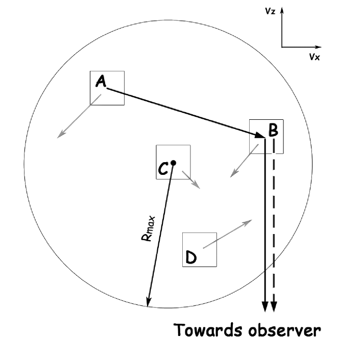
Figure 1: Geometry of the problem. Top panel: squares show different gas lumps located in one $(x,z)$ plane. Line of sight is along $z$-axis. Grey arrows show the projection of gas lump velocities onto this plane. The dashed arrow shows a photon emitted towards the observed from a gas lump B. Solid black arrows show a photon which was emitted in lump A and subsequently scattered towards the observer in lump B. The efficiency of photon scattering depends on the gas density and temperature, on the line broadening and on the relative velocities of the lumps along the direction between the lumps. The motion of a given gas lump along the line of sight (${\it v}_{Z}$) affects the observed energy of the lines , while the motion perpendicular to the line of sight (i.e. ${\it v}_{X}$ and/or ${\it v}_{Y}$) affects both direction and degree of polarization (see also Fig. 2). The ${\it v}_{Z}$ component also affects the poalrization degree by means of transverse Doppler effect, but much less than the other two components, therefore, we neglect this. Bottom panel: Line profiles in the reference system of lump B. The rest energy of the line is 6.7 keV. The energy dependent scattering cross section is schematically shown as a negative Gaussian and is marked with “B”. Emission spectra coming from lumps A, C and D are marked as “A”, “C”, and “D” respectively. The quadrupole asymmetry needed for polarization arises both due to variations of the total line flux coming to lump B from different directions and due to the Doppler shift of the lines caused by the differential bulk motions of the lumps.

The continuum emission from hot gas in galaxy clusters is optically thin. However at the energies of strong resonant transitions, the gas can be optically thick (Gilfanov, Sunyaev & Churazov, 1987). Oscillator strengths of resonant lines are large and if ion concentrations along the line of sight are sufficient, photons with energies of the resonant lines will be scattered. The geometry of the problem is sketched in Fig.1 (top panel) - from any gas lump we observe both direct (thick dashed line) and scattered (thick solid black line) emission.

If there is an asymmetry in the radiation field (in particular, a quadrupole moment) then the scattering emission will be polarized. This asymmetry can be i) due to the centrally concentrated gas distribution and ii) owing to differential gas motions (see Fig. 1 and §2).

In clusters, polarization arises rather naturally. It is well known (Sunyaev, 1982) that the scattering of radiation from a bright central source leads to a very high (up to 66%) degree of linear polarization of the scattered radiation (for a King density distribution).

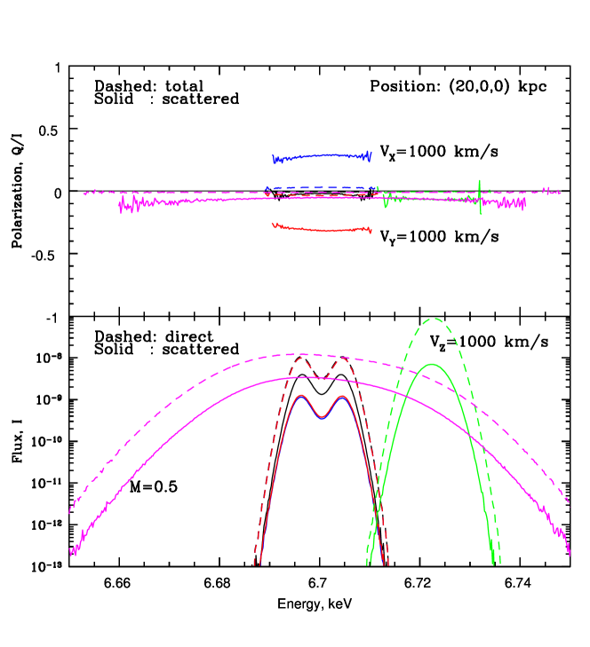
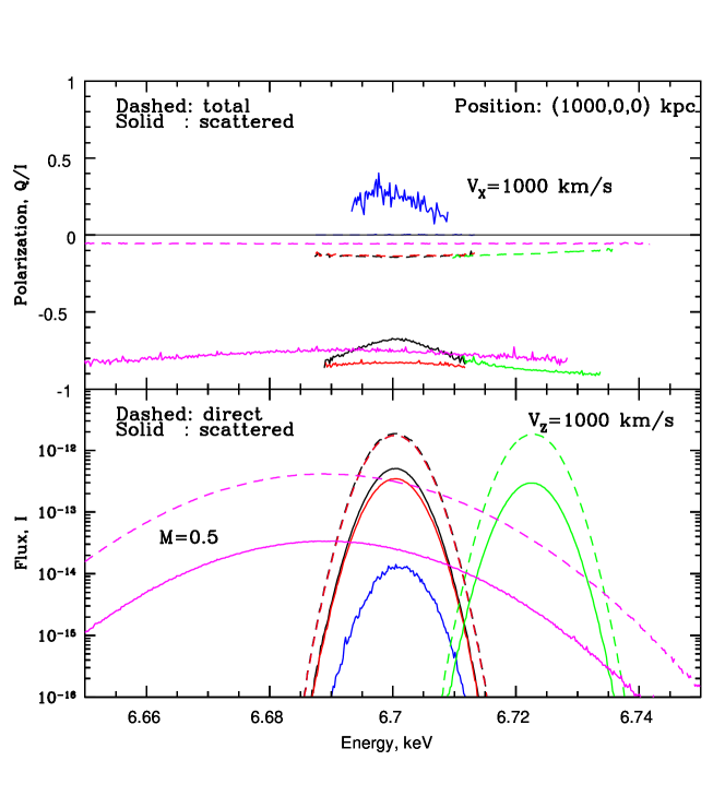
Figure 2: Line profile and polarization calculated assuming a single scattering for two small regions of a simulated galaxy cluster. Left: A region close to the cluster center with coordinates (20,0,0) kpc. $X$ and $Y$ are the coordinates in the picture plane along horizontal and vertical directions respectively, $Z$ is along the line of sight. In the bottom panel dashed lines show the line photons which are emitted within a given region and directly reached an observer without scatterings $I_{dir}$ (see dashed line in Fig.1). Solid lines show the emission scattered in a given region $I_{scat}$ (see solid thick black line in Fig.1). In the top panel the solid line is the polarization of the scattered flux only (i.e. $Q_{scat}/I_{scat}$), while the dashed line shows the polarization of the total emission, coming from a given region (i.e. $Q_{scat}/(I_{scat}+I_{dir})$).
Color coding:
Black – lines are broadened by thermal ion velocities only, all bulk velocities are set to zero. The characteristic depression at the line center is caused by the large depth at the center of the line. The degree of polarization is small since this region is exposed to essentially isotropic radiation.
Blue - the same as the black curves, but $X$ component of the gas velocity $v_{X}$ in a given region is set to 1000 km/s. Scattered flux decreases since along the direction of motion the line emission left the resonance. Polarization of the scattered flux is strong ($\sim$30%) in the direction perpendicular to the direction of motion.
Red - the same as the black curves, but $Y$ component of the gas velocity $v_{Y}$ in the region is set to 1000 km/s. Polarization of scattered flux is strong ($\sim$30%) with the polarization plane rotated by 90^∘compared to blue curves.
Green - the same as the black curves, but $Z$ component (along the line of sight) of the gas velocity $v_{Z}$ is set to 1000 km/s. The line energy is strongly shifted, while the polarization characteristics are similar to the case without gas motions (black curves). The larger flux of the line (compared to the case without gas motions) is due to a smaller optical depth towards the observer.
Magenta - the same as the black curves, but the gas bulk velocities are not set to zero, but are taken from simulations. The lines are broadened by micro-turbulence with the parameter $M=0.5$.
Right: the same as in the left panel for a gas lump located at (1000,0,0) kpc relative to the cluster center. An appreciable polarization signal is present even in the case of the gas with zero velocities.

X-ray line emission is strongly concentrated toward the cluster center due to the collisional nature of the emission process and the decrease of the plasma density with distance from the cluster center. Gilfanov, Sunyaev & Churazov (1987) have shown that resonance scattering will decrease the line surface brightness in cluster cores and increase the line brightness in the periphery of clusters. Sazonov, Churazov & Sunyaev (2002) have shown that this process should lead to a high degree of polarization in the resonance lines in high spectral resolution maps of galaxy clusters. For the richest regular clusters and clusters whose X-ray emission is dominated by a central cooling flow, the expected polarization degree is about $15\%$ (Sazonov, Churazov & Sunyaev, 2002).

In this paper we are interested primarily in the second possibility, i.e. in the modification of the polarization signal due to large scale gas motions. Of particular interest is the sensitivity of the polarization signal to $v_{\perp}$, the component of the velocity perpendicular to the line of sight.

Linear polarization $\propto(v_{\perp}/c)^{2}$ naturally appears as a result of scattering of unpolarized isotropic continuum radiation with a Rayleigh phase function. That is, for scattering of isotropic CMB radiation in the Rayleigh-Jeans limit the net polarization is given by ${\it P}\sim 0.1(v_{\perp}/c)^{2}\tau$ (Sunyaev & Zeldovich, 1980), where $\tau$ is the optical depth of the scattering medium. In the same paper Sunyaev and Zeldovich presented an approximate formula for the case of double scattering $P\sim 0.02-0.05(v/c)\tau^{2}$, where the coefficient depends on the gas distribution inside the cluster (it is $\sim 0.01$ for the King distribution, Sazonov & Sunyaev (1999)). Both these effects are very small. If there is an asymmetry in the initial angular distribution of radiation with the dimensionless amplitude $a$, then additional terms of order $a\times(v/c)$ can appear. But even these terms are expected to be small since the value of $v/c$ itself is of order $10^{-2}$ or less.

A much larger impact of the gas bulk motions is expected if line rather than continuum emission is considered. If gas is moving and along the direction of motion the Doppler shift of the photon energy exceeds the line width (i.e. line leaves the resonance) then no scattering occurs. This is illustrated in Fig.1. We consider several gas lumps marked as A, B, C and D having different bulk velocities. Region C correspond to the center of the cluster. Photons emitted in regions A, C and D are scattered towards the observer in the region B. Shown in the bottom panel of Fig.1 are the line profiles in the reference system of the lump B. The rest energy of the line is 6.7 keV. The energy dependent scattering cross section is schematically shown as a negative Gaussian and is marked with “B”. Emission spectra coming from lumps A, C and D are marked as “A”, “C”, and “D” respectively. It will be observed (§2) that a quadrupole asymmetry in the scattered radiation is needed to produce net polarization. This asymmetry arises both due to variations of the line flux coming to lump B from different directions and due to Doppler shift of the photon energies caused by the differential bulk motions of the lumps. Indeed total (integrated over energies) line flux coming from region C is the largest because of the high gas emissivity in the cluster center. At the same time, gas lump A is moving away from lump B. Therefore, in the frame of lump B, the line profile is shifted towards lower energies. The line coming from lump D is, on the contrary, shifted towards higher energies. A comparison with the energy dependent scattering cross section clearly shows that asymmetry in the scattered emission coming from different directions (and therefore the polarization) is affected by the gas velocities. What matters is the relative velocity of the gas lumps projected onto the line connecting the lumps. For example, if lump B and C are only slowly moving towards (or away) from each other then line photons coming from region C will be effectively scattered in lump B and these photons will dominate in the scattered flux seen by the observer. If on the contrary lumps B and C are approaching each other (or receding) with the velocity larger than the width of the line profile then the lump B will not scatter photons coming from C and photons coming from other direction will dominate in the scattered flux. Therefore the intensity and polarization of the scattered flux will be different for these two cases. The mutual position of lumps B and C sketched in Fig.1 shows that the polarization signal is in particular sensitive to the velocity component of lumps B and C along the X-axis, i.e. perpendicular to the line of sight.

In general relative velocities of any two gas lumps affect the polarization. However, the central region of the cluster is very bright and therefore the motion of any gas lump relative to the center is the most important, since a large fraction of scattered photons were originally born near the cluster center. If the gas density rapidly drops off with radius then the largest contribution to the scattered flux (and hence to polarization) is provided by the regions along the line-of-sight which are most close to cluster center – not far from the picture plane going though the center. Thus, the scattering by $\sim$90^∘is the most important, i.e. photons, emitted in the cluster center, scatter in gas lump in the picture plane and then come to observer. In this case the velocities perpendicular to the line-of-sight affect the scattering and polarization most strongly. Of course, in real systems different scattering angles make contributions to the scattered flux and therefore gas motions in different directions play a role. Below (Section 5) we make a full accounting of 3D velocity field using numerical simulations of galaxy cluster and take into account relative motions of the gas lumps in all directions.

At the same time, the presence of gas motions along the line of sight leads to strong fluctuations of the centroid energy and the shape of the resonant lines (see Inogamov & Sunyaev, 2003) and can be measured with high resolution spectrometers.

One can also consider the impact of small-scale random (turbulent) gas motions on the line profiles and the polarization signal. As has been shown by Gilfanov, Sunyaev & Churazov (1987), micro-turbulence makes the lines broader, decreasing the optical depth and therefore reducing the effects of resonant scattering and polarization. They pointed out that in galaxy clusters the effect is especially strong for heavy elements, which have thermal velocities much smaller than the sound velocity of the gas. For example, for the 6.7 keV iron line in the spectrum of the Perseus cluster, the inclusion of turbulent motions would reduce the optical depth from $\sim 2.8$ to $\sim 0.3$ for a Mach number of 1 (Churazov et al., 2004). Turbulent motions were also considered in the dense cores of X-ray halos of giant elliptical galaxies. Werner et al. (2009) placed tight constraints on turbulent velocities from the effect of resonant scattering on the ratio of optically thin and thick lines. They have shown that characteristic turbulent velocities in the center of the giant elliptical galaxy NGC4636 are less than 100 km/s.

These points are illustrated in Fig.2 where the spectra and the polarization signal coming from two gas clumps in a simulated galaxy cluster are shown. Here we are using a model cluster as described in section 5. All calculations for this plot were done assuming a single-scattering by 90^∘. The left panel shows the radiation emerging from a region close to the cluster center. Due to it’s central location, the incident radiation field is almost isotropic and the resulting polarization signal is week. Adding bulk motions in the picture plane ($v_{x}$, $v_{y}$ - blue and red lines, respectively) immediately produces polarization in the perpendicular direction, but does not affect the line shape. On the contrary, adding a line-of-sight velocity component ($v_{z}$ - green line) shifts the line energy, but does not affect the polarization signal. Finally, adding micro-turbulence makes the line broader. The right panel of Fig.2 shows the same effects for a small region located in the cluster outskirts. For this region, the asymmetry in the incident radiation is already present and non-zero polarization is expected even without gas motions. Adding velocity in the “horizontal” direction changes the sign of the polarization signal.

Thus combining the data from high resolution X-ray spectrometers and X-ray polarimeters, one can constrain both line-of-sight and perpendicular components of the velocity field - an exercise hardly possible to do by any other means.

The structure of the paper is as follows. In Section 2 we discuss main criteria for selection of X-ray emission lines, most promising for polarization studies. In Section 3 we describe a Monte Carlo code used to simulate resonant scattering. Two characteristic flow patterns (a canonical cooling flow and an expanding spherical shock) in the approximation of a spherical symmetry are considered in Section 4. In Section 5 we present the results of resonant scattering simulations in full 3D geometry, using several clusters taken from cosmological simulations. The calculations described in Sections 4 and 5 take into account only line photons. In Section 6 we summarize our results, discuss additional effects which reduce the polarization degree in galaxy clusters – the most most important one is the contamination of the polarized line flux with unpolarized continuum and line emission from the thermal plasma. Finally in Section 7 we outline requirements for future X-ray polarimeters.

2 Resonant scattering and promising lines

For the most prominent lines (e.g. 6.7 keV line of He-like iron) the scattering is characterized by the Rayleigh phase function similar to the scattering phase function by free electrons.

If $E$ is the photon energy, $E_{0}$ is the energy of the transition (line), v is the gas bulk velocity, m is the photon propagation direction, $\sigma$ is the Gaussian width of the line set by thermal broadening and micro-turbulent gas motions. The cross section for resonant scattering in the lines in the rest frame of a given gas lump is a strong function of energy

$$s\propto\displaystyle e^{-\frac{\left(E\left[1-({\bf vm})/c\right]-E_{0}\right)^{2}}{2\sigma^{2}}}.$$ (1)

If $\mu=\cos\theta$, where $\theta$ and $\phi$ are the polar angles in the frame set by the photon direction of propagation after scattering, $I(E,\mu,\phi)$ is the initial unpolarized radiation, $\sigma_{0}$ is the scattering cross section by one ion and $n_{i}$ is the number density of corresponding ions, then according to Chandrasekhar (1950), one can write a simple expression for the integrated energy flux scattered in a small volume of gas $dV$ and for the Stokes parameter $Q$:

$$I_{scat}=\sigma_{0}n_{i}dV\int e^{-\frac{\left(E\left[1-({\bf vm})/c\right]-E_{0}\right)^{2}}{2\sigma^{2}}}\times$$

$$\frac{3}{16\pi}(1+\mu^{2})~{}I(E,\mu,\phi){\rm d}\mu{\rm d}\phi{\rm d}E$$

$$Q=\sigma_{0}n_{i}dV\int e^{-\frac{\left(E\left[1-({\bf vm})/c\right]-E_{0}\right)^{2}}{2\sigma^{2}}}\times$$

$$\frac{3}{16\pi}(\mu^{2}-1)\cos 2\phi~{}I(E,\mu,\phi){\rm d}\mu{\rm d}\phi{\rm d}E.$$ (2)

The presence of the term $(\mu^{2}-1)\cos 2\phi$ in the expression for $Q$ shows that net polarization arises when an angular function

$$F(\mu,\phi)\equiv\displaystyle\int e^{-\frac{\left(E\left[1-({\mathbf{v}\mathbf{m}})/c\right]-E_{0}\right)^{2}}{2\sigma^{2}}}I(E,\mu,\phi){\rm d}E$$ (3)

has non-zero quadrupole moment. As discussed in §1 this quadrupole moment can arise due to the asymmetry in $\int I(E,\mu,\phi)dE$ and/or by angular dependence in the cross section $s(E,\mu,\phi)$ caused by the factor $({\mathbf{v}\mathbf{m}})/c$. Note that in the bottom panel of Fig. 1 all profiles are plotted in the rest frame of a given gas lump, while the above expressions are written in the laboratory frame.

The optical depth of a line is defined as

$$\tau=\int\limits_{0}^{\infty}n_{\rm i}\sigma_{0}{\rm d}r,$$ (4)

where $n_{i}$ is the ion concentration and $\sigma_{0}$ is the cross section at the center of the line

$$\sigma_{0}=\frac{\sqrt{\pi}hr_{\rm e}cf}{\Delta E_{\rm D}},$$ (5)

where $r_{\rm e}$ is the classical electron radius and $f$ is the oscillator strength of a given atomic transition. In plasma with a temperature characteristic of galaxy clusters, the line width is determined by the velocities of thermal and turbulent motions, rather than by the radiative width. The Doppler width of the line is defined as

$$\Delta E_{\rm D}=E_{0}\left[\frac{2kT_{\rm e}}{Am_{\rm p}c^{2}}+\frac{V_{\rm turb}^{2}}{c^{2}}\right]^{1/2},$$ (6)

where $A$ is the atomic mass of the corresponding element, $m_{\rm p}$ is the proton mass and $V_{\rm turb}$ is the characteristic turbulent velocity. $V_{\rm turb}$ is parametrized as $V_{\rm turb}=c_{\rm s}M$, where $M$ is the Mach number and the sound speed in the plasma is $c_{\rm s}=\sqrt{\gamma kT/\mu m_{\rm p}}$, where $\gamma=5/3$ is the adiabatic index for an ideal monoatomic gas and $\mu=0.62$ is the mean atomic weight. We can rewrite the previous expression as

$$\Delta E_{\rm D}=E_{0}\left[\frac{2kT_{\rm e}}{Am_{\rm p}c^{2}}(1+1.4AM^{2})\right]^{1/2}.$$ (7)

It is clear from the above expressions that to have large optical depth in the line, the oscillator strength has to be large. If the line width is dominated by thermal broadening then the lines of the heaviest elements will be narrower than for the lighter elements, and the optical depth for lines of heavy elements will be larger as well.

Resonant scattering can be represented as a combination of two processes: isotropic scattering with a weight $w_{1}$ and dipole (Rayleigh) scattering with weight $w_{2}=1-w_{1}$ (Hamilton, 1947; Chandrasekhar, 1950). Weights $w_{1}$ and $w_{2}$ depend on the total angular momentum $j$ of the ground level and on the difference between the total angular momentums of excited and ground levels $\Delta j$ (=$\pm 1$ or $0$). The expressions for the weights were calculated by Hamilton (1947). Isotropic scattering introduces no polarization, while Rayleigh scattering changes the polarization state of the radiation field. Therefore, to have noticeable polarization, we have to select lines with a large optical depth and with large Rayleigh scattering weight $w_{2}$.

In the spectrum of a typical rich cluster of galaxies, often the strongest line is the He-like K_α line of iron with rest energy 6.7 keV. Ions of He-like iron are present in plasma with temperature in the range from $\sim$1.5 to $\sim$10 keV. The transition $1s^{2}(^{1}S_{0})-1s2p(^{1}P_{1})$ of He-like iron has an absorption oscillator strength $\sim 0.7$ and we can expect this line to be optically thick, leading to a significant role of resonant scattering. Also this transition corresponds to the change of the total angular momentum from 0 to 1 and according to Hamilton (1947) the scattering has a pure dipole phase function. So, we can expect a high degree of polarization in this line. In the vicinity of this resonant line there are intercombination ($1s^{2}(^{1}S_{0})-1s2p(^{3}P_{1,2})$), forbidden ($1s^{2}(^{1}S_{0})-1s2s(^{3}S_{1})$) lines of He-like iron and many satellite lines. Forbidden and intercombination lines have an absorption oscillator strength at least a factor 10 smaller than the resonant line (Porquet et al., 2001) and a small optical depth accordingly. Satellite lines correspond to the transitions from excited states and in the low density environment have negligible optical depth.

In cooler clusters with temperatures below 4 keV, the Li-like iron is present in sufficient amounts and the Fe XXIV line $1s^{2}2s(^{2}S_{1/2})-1s^{2}3p(^{2}P_{3/2})$ at 1.168 keV is especially strong. The dipole phase function has a weight of 0.5 for this line.

At even cooler temperatures $\sim 1~{}{\rm keV}$ the most promising line for polarization studies is the Be-like line ($1s^{2}2s(^{1}S_{0})-1s^{2}2s3p(^{1}P_{1})$) of iron with rest energy 1.129 keV, which has an oscillator strength 0.43 and a unit weight of dipole scattering. Other lines are discussed in detail by Sazonov, Churazov & Sunyaev (2002).

3 Monte-Carlo simulations

We performed two types of numerical simulations for two different initial conditions:

• spherically symmetric clusters.

• full three-dimensional galaxy cluster models, taken from cosmological large-scale structure simulations.

3.1 Spherically symmetric clusters

In the spherically symmetric simulations, we describe a cluster as a set of spherical shells with given densities, temperatures and radial velocities. To calculate plasma line emissivities we use the Astrophysical Plasma Emission Code (APEC, Smith et al. (2001)). Line energies and oscillator strengths are taken from ATOMDB and the NIST Atomic Spectra Database. The ionization balance (collisional equilibrium) is that of Mazzotta et al. (1998) - the same as used in APEC.

Multiple resonant scattering is calculated using a Monte-Carlo approach (see e.g. Pozdnyakov, Sobol, & Sunyaev, 1983; Sazonov, Churazov & Sunyaev, 2002; Churazov et al., 2004). We start by drawing a random position of a photon within the cluster, random direction of the photon propagation ${\mathbf{m}}$ and the polarization direction ${\mathbf{e}}$, perpendicular to ${\mathbf{m}}$. The photon is initially assigned a unit weight $w$. Finding an optical depth $\tau$ in the direction of photon propagation up to the cluster edge and an escape probability $p_{\rm esc}=e^{-\tau}$, we draw the optical depth of the next scattering as $\tau_{\rm next}=-\ln(1-\xi(1-p_{\rm esc}))$, where $\xi$ is a random number distributed uniformly on the interval $[0,1]$. Using the value of $\tau_{\rm next}$ the position of the next scattering is identified. The code allows one to treat an individual act of resonant scattering in full detail. The phase function is represented as a combination of dipole and isotropic scattering phase matrixes with weights $w_{1}$ and $w_{2}$. In the scattering process the direction ${\bf m^{\prime}}$ of the emerging photon is drawn in accordance with the relevant scattering phase matrix. For an isotropic phase function, the new direction ${\bf m^{\prime}}$ is chosen randomly. For a dipole phase function, the probability of the emerging photon to have new direction ${\bf m^{\prime}}$ is $P({\bf m^{\prime}},{\bf e^{\prime}})\propto\displaystyle({\bf e^{\prime}},{\bf e})^{2}$, where the electric vector ${\bf e^{\prime}}=\displaystyle\frac{{\bf e}-{\bf m^{\prime}}\cos\alpha}{\sqrt{1-\cos^{2}\alpha}}$ and $\alpha$ is an angle between the electric vector ${\bf e}$ before scattering and the new direction of propagation ${\bf m^{\prime}}$, i.e. $\cos\alpha=({\bf e},{\bf m^{\prime}})$. For the energy of the photon, we assume a complete energy redistribution. After every scattering, the photon weight $w$ is reduced by the factor $(1-e^{-\tau})$. The process repeats until the weight drops below the minimal value $w_{min}$. Thus, specifying the minimum photon weight, we can control the number of multiple scatterings. A typical value of the minimum weight used in the simulations is $w_{min}=10^{-9}$.

After every scattering for a photon propagating in the direction ${\mathbf{m}}$, a reference plane perpendicular to ${\mathbf{m}}$ is set up for Stokes parameter calculations. One of the reference axes is set by projecting a vector connecting the cluster center and the position of the last scattering on the reference plane. The Stokes parameter $Q$ is defined in such a way that it is non-zero when the polarization is perpendicular to the radius. From the symmetry of the problem, it is obvious that the expectation value of the $U$ parameter in our reference system is $\equiv 0$. Then the projected distance $R$ from the center of the cluster is calculated and the Stokes parameters $I$ and $Q$ are accumulated (as a function of $R$) with the weight $\propto\epsilon\times w\times e^{-\tau}$, where $\epsilon$ is the volume emissivity at the position where the initial photon was born. Finally the degree of polarization is calculated as $P(R)=Q(R)/I(R)$.

Table 1: Oscillator strength and optical depth of the most promising X-ray lines in Virgo/M87 and Perseus clusters.

Ion	$E,~{}{\rm keV}$	$f$	$w_{2}$	$\tau$, Virgo/M87	$\tau$, Perseus
Fe XXII	1.053	0.675	0.5	0.65	0.02
Fe XXIII	1.129	0.43	1	1.03	0.16
Fe XXIV	1.168	0.245	0.5	1.12	0.73
Si XIV	2.006	0.27	0.5	0.6	0.24
S XV	2.461	0.78	1	0.68	0.03
Fe XXV	6.7	0.78	1	1.44	2.77
Fe XXV	7.881	0.15	1	0.24	0.45

3.2 Full 3D clusters

In the full 3D simulations, cluster parameters (gas density and temperature) are computed on a 3D Cartesian grid and the velocity field is represented as a 3D vector field. In contrast to a symmetric code, the 3D code precisely takes into account the changes of photon energy due to scattering, assuming Gaussian distributions of thermal and turbulent ion velocities.

For every simulation we choose the viewing direction and setup a reference system in the plane, perpendicular to the viewing direction. The Stokes parameters $I$, $Q$ and $U$ are calculated with respect to this reference system and are accumulated in a form of 2D images. Finally the degree of polarization is calculated as $P=\sqrt{Q^{2}+U^{2}}/I$.

4 Spherically symmetric problems

We have performed spherically symmetric calculations to simulate resonant scattering polarization effects in two galaxy clusters: Perseus and Virgo/M87, as examples of cooling flow clusters.

4.1 Perseus cluster

Figure 3: Top panel: polarization degree as a function of projected distance from the center of the Perseus cluster in the most prominent resonant line of Fe XXV with energy 6.7 keV, assuming flat iron abundance (the thick solid curve). Other thin curves show results of calculations done for different sizes of the cluster (maximal radius $r_{\rm max}$) assumed in the simulations: the upper dot-dashed curve for $r_{\rm max}=1000$ kpc, the dashed curve is for $r_{\rm max}=1400$ kpc, the dotted line is for $r_{\rm max}=3000$ kpc and the lower dot-dashed line for the cluster size $r_{\rm max}=4000$ kpc. Clearly the polarization degree in the cluster outskirts strongly depends on the assumed extent of the cluster. For reference, the virial radius of the Perseus cluster is $r_{200}\approx 2100$ kpc. Depending on $r_{\rm max}$ the degree of polarization at a distance of 1 Mpc can vary from 8 to 12%. At smaller distances the degree of polarization is less sensitive to the cluster properties at large radii. Thick long dashed curve shows polarization degree in the case of peaked abundance.
Bottom panel: simulated surface brightness of Perseus in the 6.7 keV line, calculated with and without resonant scattering - dashed and solid lines, respectively. Resonant scattering diminishes the flux in the cluster center and increases the flux at larger radii.

Figure 4: Top panel: polarization degree as a function of projected distance from the center of the Virgo/M87 cluster in the most prominent resonant lines, presented in Table LABEL:tab:lines.
Bottom panel: simulated surface brightness on the Virgo/M87 cluster in the lines presented on the top panel. Scattering is included.

The electron density distribution for the Perseus cluster was adopted from Churazov et al. (2003). They describe the density profile as a sum of two $\beta-$models and they assume a Hubble constant of $50~{}\rm{km/s/Mpc}$. Correcting the density distribution to the value of the Hubble constant $H_{0}=72~{}{\rm km/s/Mpc}$ we find

$$n_{e}=\frac{4.68\times 10^{-2}}{\left[1+\left(\frac{r}{56}\right)^{2}\right]^{\frac{3}{2}\times 1.2}}+\frac{4.86\times 10^{-3}}{\left[1+\left(\frac{r}{194}\right)^{2}\right]^{\frac{3}{2}\times 0.58}}~{}~{}~{}{\rm cm}^{-3}$$ (8)

The temperature distribution is described as

$$T_{e}=7\frac{\left[1+\left(\frac{r}{100}\right)^{3}\right]}{\left[2.3+\left(\frac{r}{100}\right)^{3}\right]}~{}~{}~{}{\rm keV},$$ (9)

where $r$ is measured in kpc.

The iron abundance is assumed to be constant over the whole cluster and equal to 0.5 solar using the Anders and Grevesse abundance table (Anders & Grevesse, 1989). This value is equivalent to 0.79 solar if the newer solar photospheric abundance table of Lodders (2003); Asplund, Grevesse, & Jacques Sauval (2006) is used.

Sazonov, Churazov & Sunyaev (2002) produced a list of the strongest X-ray lines in the Perseus cluster with optical depth $\tau>0.5$. Only three lines have dipole scattering weight larger than the weight of isotropic scattering: the He-like K_α line with energy 6.7 keV, the He-like K_β line ($1s^{2}-1s3p(^{1}P_{1})$) at 7.88 keV and the L-shell line of Li-like iron with energy $1.168~{}{\rm keV}$. The optical depths of these lines are $\sim 3$, $\sim 0.45$ and $\sim 0.73$ respectively (see Table LABEL:tab:lines). Therefore, for the Perseus cluster we performed calculations for the permitted line at 6.7 keV as the optical depth in this line is the largest, weight $w_{2}=1$, and hence the polarization of scattered radiation in this line is expected to be the most significant.

4.2 M87/Virgo cluster

Another example of a cooling flow cluster is the M87/Virgo cluster. In this cluster the temperature in the center is lower than in Perseus. The temperature and number electron density profiles in the inner region were taken from Churazov et al. (2008). The electron density is described by $\beta$-law distribution with

$$n_{e}=\frac{0.22}{\left[1+\left(\frac{r}{0.93}\right)^{2}\right]^{\frac{3}{2}\times 0.33}}~{}~{}~{}{\rm cm}^{-3},$$ (10)

where $r$ is in kpc. Temperature variations can be approximated as

$$T=T_{0}\left[1+\left(\frac{r}{r_{\rm c}}\right)^{2}\right]^{0.18},$$ (11)

where the central temperature is parameterized by $T_{0}=1.55~{}{\rm keV}$ and $r_{\rm c}=10.23~{}{\rm kpc}$. In clusters with such low central temperatures the lines of Li-like and Be-like iron become very strong. In Table LABEL:tab:lines we list potentially interesting lines in M87, which have weight $w_{2}\geq 0.5$. The most interesting lines are those at 1.129 keV and at 6.7 keV as the optical depth is large and the scattering phase function is pure dipole. Also notable are the lines of Li-like iron at 1.168 keV and line of S XV at 2.461 keV, which have weights $w_{2}=0.5$ and $w_{2}=1$ respectively. The line at 1.168 keV has two components. The first component has zero weight of dipole scattering, while the second at 1.168 keV has equal weights of dipole and isotropic scattering. Therefore, we consider only the second component in our simulations.

The Fe and S abundances are assumed to be constant at $r<10$ kpc, being Z(Fe)=1.1 and Z(S)=1 (relative to the solar values of Lodders (2003)), then gradually falling with radius to reach the values Z(Fe)=0.56 and Z(S)=0.63 at $r=40$ kpc, and remain constant from there on. These approximations are in a good agreement with observations (e.g. Werner et al., 2006).

One can notice, that optical depths, presented in Table LABEL:tab:lines, are systematically lower than in Sazonov, Churazov & Sunyaev (2002). This is caused by differences in number density and temperature profiles. We are using newer profiles and, for example, in case of Virgo cluster number density is systematically lower and temperature in center is higher, leading to the changes in ion fractions. All this factors together reduce the optical depths of lines.

4.3 Degree of polarization without bulk motions

In Fig.3 the results for the Perseus cluster are shown. As already discussed the calculations were done for the He-like K_α line at 6.7 keV. The polarization is zero at the center of the cluster (as expected from the symmetry of the problem) and increases rapidly with increasing distance from the center. At large distances from the center the degree of polarization depends strongly on the maximum radius $r_{\rm max}$ used in the simulations. This is an expected result. Indeed for steep density profiles at the periphery of a cluster the largest contribution to the scattered signal is due to small region along the line-of-sight (near the closest approach to the cluster center). Since most of the photons are coming from the central bright part of the cluster, the role of 90^∘scatterings increases. Recall that for the Rayleigh phase function, 90^∘scattering produces 100% polarized radiation. Therefore near the edges of the simulated volume the degree of polarization is expected to increase, even although the polarized scattered radiation will always be diluted by locally generated line photons. Obviously the final value of polarization degree at a given projected radius depends also on the cluster properties at larger radii. The virial radius of the Perseus cluster is $r_{200}\approx 2.1$ Mpc. Our simple approximations for the gas density and temperature certainly break there (perhaps at a fraction of the virial radius). Nevertheless, the gas beyond virial radius has a very low density and it is likely not hot enough to produce strong emission in the 6.7 keV line. From this point of view an effective cut-off radius $r_{\rm max}$ in the gas distribution may suffice as an illustration of the polarization signal sensitivity to the structure of the cluster outskirts. In Perseus simulations as $r_{\rm max}$ varies from 1 Mpc to 4 Mpc (Fig.3, the top panel), i.e. the boundary of the simulated volume extends to larger distances, the degree of polarization at the projected distance of 500 kpc decreases from $\sim$8 to 7%. At the very edge of the cluster one can expect the maximum degree of polarization in the Perseus cluster of order 10% . Also shown in Fig.3 are the surface brightness profiles in the 6.7 keV line, calculated with and without resonant scatterings (the bottom panel).

As already mentioned above, a flat abundance profile ($Z=0.79$) was assumed in these calculations. We also tried a peaked abundance profile based on the XMM-Newton observations of the Perseus cluster (Churazov et al., 2003): the iron abundance is $\sim 1.1$ in the center ($r<60$ kpc), gradually decreases to $\sim 0.7$ at $r\sim 200$ kpc and is flat at larger radii. The polarization degree, corresponding to the peaked abundance profile is shown in Fig.3 with the thick long dashed curve. In general the agreement with the calculations for a flat abundance profile is good. The maximum polarization does not change, while at distances $r<200$ kpc a small bump in polarization degree appears. At $r=100$ kpc the polarization degree increases from $5\%$ to $6\%$, staying constant till 200 kpc. We further discuss the effect of the peaked abundance profile in Section 5.

Figure 5: Inflow velocity $v_{\rm r}$ in homogeneous cooling flow models for Perseus (thick lines) and Virgo (thin lines). The solid lines show the radial velocities estimated from eq.(12) and the dashed lines show velocities calculated from eq.(13). The cooling rates for Perseus and Virgo are assumed to be constant and are 183 M${}_{\odot}/{\rm yr}$ and 10 M${}_{\odot}/{\rm yr}$ correspondingly.

Fig.4 (top panel) shows the simulated radial profiles of the degree of polarization for Virgo in several prominent lines. The highest polarization is achieved in the Fe XXIII 1.129 keV line, reaching a maximum of 3.5$\%$ at the distance $\sim$15 kpc from the center and falling off from this maximum with increasing distance from the center. A similar behaviour pertains for the lines at 1.168 keV and 2.461 keV. In spite of higher optical depth of line at 1.168 keV, the polarization is lower due to the smaller weight of dipole scattering. It is also important to note that close to the 1.168 keV line there is a second component at 1.163 keV, which produce unpolarized emission and contaminate polarized signal from 1.168 keV line unless the energy resolution is better that 5 keV. Polarization in the line of He-like (at 6.7 keV) iron increases slowly with projected radius and is of order 1%. Surface brightness profiles are also shown on the Fig.4 (bottom panel) for all lines shown on the upper panel. We see that lines of Fe XXIII and S XV have not only the largest polarization degree, but also the largest intensity in Virgo cluster.

Comparing profiles of the polarization degree in Perseus and M87 one can notice a different behavior of the curves: in Perseus cluster the polarization is an increasing function of radius, while in M87/Virgo cluster the degree of polarization decreases with radius. This is caused by different radial behavior of the density profiles, since the polarization degree strongly depends on the $\beta$-parameter. It is clear, that the polarization degree is smaller for smaller $\beta$, since for small $\beta$ the cluster emission becomes less centrally peaked, leading to a more isotropic radiation field. According to the analytical solution given by Sazonov, Churazov & Sunyaev (2002), at large distances from the cluster center $\displaystyle P=Q/I\propto\frac{r^{-3\beta-1}}{r^{-6\beta+1}}=r^{3\beta-2}$. It is clear that if $\beta>2/3$ (case of the Perseus cluster) the polarization degree will increase with distance, while if $\beta<2/3$ (case of the M87/Virgo cluster) emission is less peaked and the polarization degree diminishes far from the cluster core.

4.4 Canonical cooling flow model

The polarization degree was calculated for several patterns of gas motions. First we consider a canonical cooling flow model (a slow flow of cooling gas toward the center of the cluster). While we understand the canonical cooling flow model has now been transformed into a picture of feedback from central supermassive black holes, the model provides a baseline for exploring symmetric gas flows. The velocity of the flow can be estimated, assuming that the flow time is approximately equal to the cooling time:

$$r/v\approx t_{\rm cool},$$ (12)

where $\displaystyle t_{\rm cool}=\frac{5/2nkT}{n^{2}\Lambda(T)}$, $n$ is the gas density, and $\Lambda(T)$ is the gas cooling function. The radial velocities estimated from eq. (12) using the observed temperature and density profiles in Perseus and M87 are shown in Fig.5 with solid lines. In both clusters the velocities are very small and do not exceed 30 ${\rm km~{}s^{-1}}$.

Larger velocities are anticipated in a homogeneous cooling flow model which assumes that the mass flow rate is constant at all radii: $\displaystyle\dot{M}_{\rm cool}(r)=4\pi r^{2}\rho v_{\rm r}={\rm const}$. Sarazin (1996) provides the following estimate of the inflow velocity for such a model:

$$v_{\rm r}=9\left(\frac{r}{100kpc}\right)^{-1/2}\times$$

$$\left[\frac{\dot{M}_{\rm cool}(r)}{300M_{\odot}yr^{-1}}\right]^{1/2}\left[\frac{T(r)}{10^{8}K}\right]^{-1/2}~{}~{}~{}~{}{\rm km~{}s^{-1}}.$$ (13)

According to Fabian (1994) the cooling rates in M87 and Perseus are 10 M${}_{\odot}{\rm/yr}$ and 183 M${}_{\odot}{\rm/yr}$ respectively. The radial velocities in Perseus and M87, estimated from eq.(13) using the observed temperature profiles, are shown in Fig.5 with the dashed lines. Even if velocities are calculated using eq.(13) they are not large: at a distance of 1 kpc from the center they are about 30 km/s for M87 and about 100 km/s for the Perseus cluster.

Figure 6: Density, temperature and gas velocity profiles in 1D simulations of an expanding shock wave produced by an AGN outburst in the giant elliptical galaxy M87 with the total energy release of $E_{0}\sim 5\times 10^{57}{~{}~{}\rm ergs}$ and the duration of the outburst $\Delta t\sim 2\times 10^{6}{~{}~{}\rm yr}$ (Forman et al., 2009). Dotted lines show the assumed initial density and temperature distributions. Solid lines in each panel show the density, temperature and velocity distributions about 12 Myr after the beginning of the outburst.

Inclusion of velocities of cooling flows does not change the degree of polarization in either M87 or Perseus since the flow velocities are small. The only appreciable effect is in the very central parts of the clusters (Fig.5) where the degree of polarization is very small anyway, with or without the flow.

4.5 Spherical shock model

Figure 7: Top panel: surface brightness profile in the resonant K_α line of He-like iron at 6.7 keV for Virgo/M87. The dashed curves correspond to the initial temperature and electron number density distributions and the solid curves are for the case of a propagating shock wave. Here, the upper curves (dashed and solid) show profiles without scattering while the other two curves show surface brightness taking into account scattering.
Bottom panel: expected degree of polarization in the 6.7 kev line. The dashed curve corresponds to the initial gas density and temperature distributions without the shock. The solid curve corresponds to the density, temperature and velocity profile expected in the case of a Mach 1.2 shock at r=13 kpc propagating through the ICM. The dashed-dotted line correspond to the same case, but with the gas velocity set to zero. The differences between the last two profiles is not large. Therefore, changes in polarization degree are most sensitive to changes in number density and temperature profiles, rather than to the gas velocity.

As another possible pattern of gas motions, we consider an expanding spherical shock, using M87 as an example (Forman et al., 2005, 2007). This can be considered as a prototypical case of a cool core cluster, albeit less luminous than the Perseus cluster. All cool core clusters contain a supermassive black hole (an AGN) in a giant elliptical galaxy at the cluster center which is believed to be the source of energy for the cooling gas. AGN activity is also a natural candidate for generation of gas motions: it can either cause turbulent motions by stirring the gas or produce larger scale gas motions in a form of an expanding shock wave. Following Forman et al. (2007, 2009), we used 1D simulations of an expanding shock in M87, which is produced by the AGN outburst with the total energy release $E_{0}\sim 5\times 10^{57}{~{}~{}\rm ergs}$ and the duration of the outburst $\Delta t\sim 2\times 10^{6}{~{}~{}\rm yr}$. These parameters were derived based on the comparison of the shock simulations with the data of a 0.5 Ms long Chandra observations of M87 by Forman et al. (2007, 2009). Observed position of the shock is at $\sim 2.8^{\prime}$ (13 kpc) from the center of M87 and the Mach number of the shock is $\sim 1.2$. Shown in Fig.6 are results of 1D simulations of shock propagation through the M87 atmosphere about 12 Myr after the beginning of the outburst: solid lines in each panel show the density, temperature and velocity distributions. Dotted lines show the assumed initial density and temperature distributions. The energy in the simulations was released in a small volume near the center which by the end of the simulations has expanded into a $\sim$3 kpc sphere filled with a very high entropy gas. This is of course the result of our adopted 1D geometry. In reality, the structure of the inner 3 kpc is much more complicated (see Forman et al., 2007). We expect however that our modelling of the outer part is sufficiently accurate and can be used as an illustrative example of the impact of a weak shock on the polarization signal. The gas properties (Fig.6) show all the features of a weak spherical shock, in particular a “sine-wave” structure of the velocity distribution. The maximum positive velocity (expansion) is $\sim 180~{}{\rm km~{}s^{-1}}$, while maximal negative velocity (contraction) is $\sim 60~{}{\rm km~{}s^{-1}}$.

For the Virgo cluster we then carried out three radiative transfer simulations: A) using initial undisturbed profiles (dotted lines in Fig.6), B) using density and temperature distributions as in the shock, but setting the gas velocity to zero and C) using density, temperature and velocity distributions as in the shock (solid lines in Fig.6). The reason for doing simulations B is that we want to see the impact of the nonzero velocity separately from other effects. We preformed calculations for the line with energy 6.7 keV (see Table LABEL:tab:lines) as the influence of the shock wave at such energy is more noticeable.

The results of radiative transfer calculations are shown in Fig.7. Shown in the top panel are the surface brightness profiles for cases A (the dashed curves) and B (the solid curves). Profiles in the simulation C are the same as in case B. Here, the upper lines correspond to the profiles without scattering and the lower lines show surface brightness, taking into account scattering. Due to resonant scattering the surface brightness becomes weaker in the center and stronger outside. Because of shock wave propagation the number density in the center becomes smaller leading to the lower surface brightness in the cluster center. Also, due to the shock wave, we see a characteristic peak $\sim$10 kpc from the center. Bottom panel in Fig.7 shows the polarization degree for cases A, B, C. We see that after the shock wave propagates, the gas is less dense, therefore the line has smaller optical depth and the polarization decreases. The velocities of gas are larger than in the case of cooling flows and lead again to the decrease of the polarization degree.

5 Three-dimensional problem

We now consider full three-dimensional models of galaxy clusters, taken from large-scale structure formation. The density, temperature distributions and the velocity field are taken from a set of high-resolution simulations of galaxy clusters (see e.g. Dolag et al., 2005, 2008) which are based on Gadget-2 SPH simulations (Springel, Yoshida, & White, 2001) and include various combinations of physical effects. We use the output of non radiative simulations. All data are adaptively smoothed and placed in a cube with half size 1000 kpc and cell size 3 kpc. The resonant scattering is calculated using a Monte-Carlo approach, which is described above in section 3.

We discuss here results of calculations for three simulated galaxy clusters: g6212, g72 and g8. Table LABEL:tab:clpar shows the basic parameters of the chosen clusters. The slices of the density and temperature distributions for all clusters and their projected images in X-ray lines are shown in Fig.8.

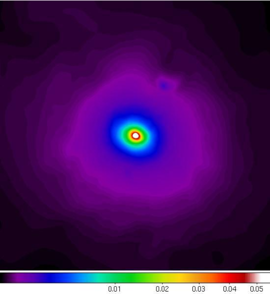
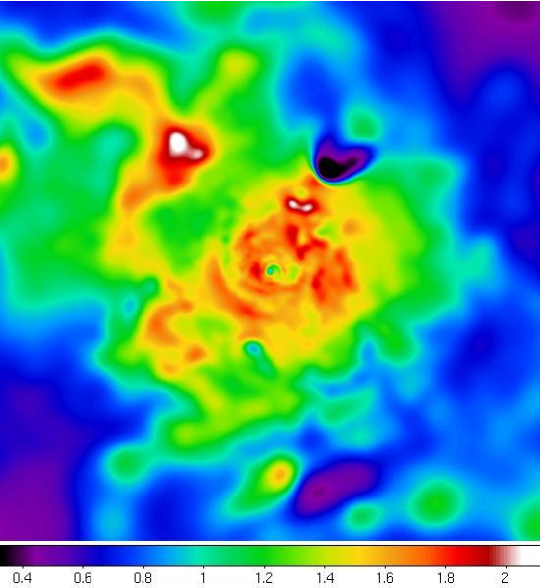
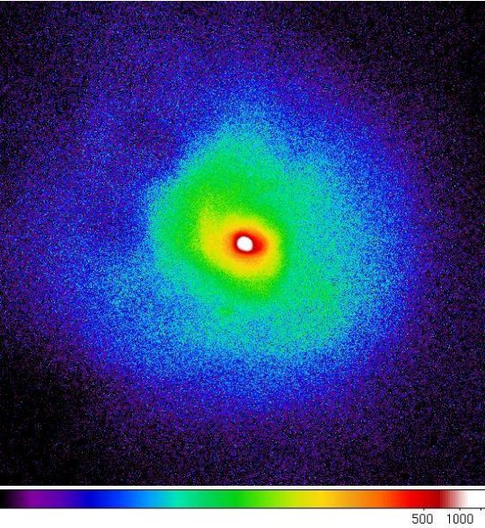
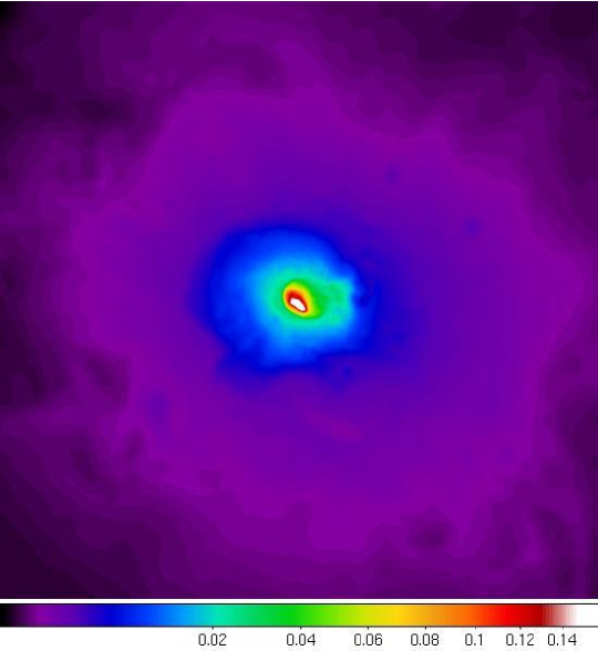
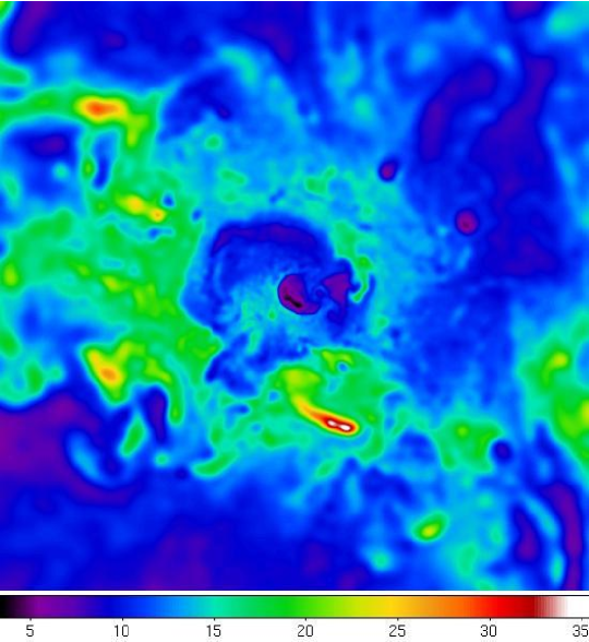
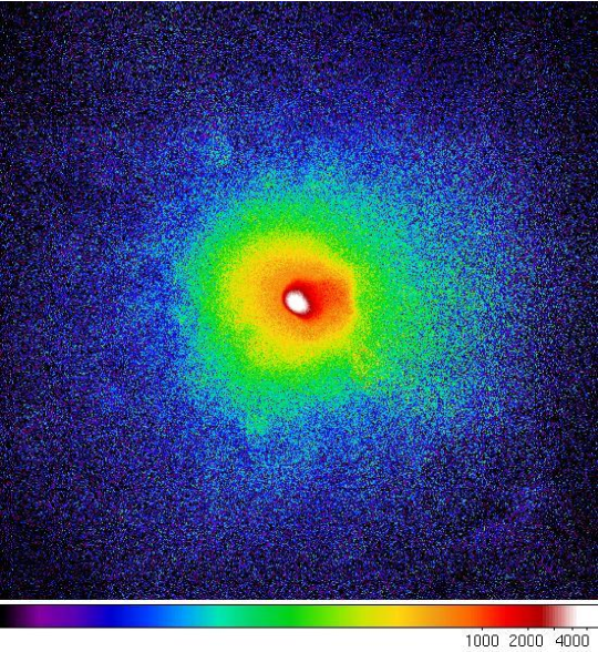
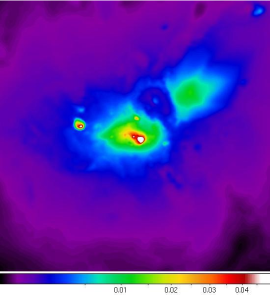
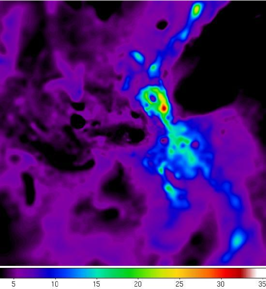
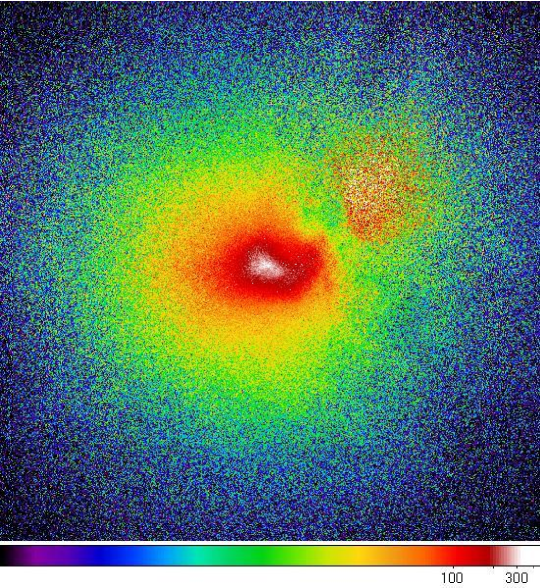
Figure 8: Simulated clusters g6212 (the top panels), g8 (the middle panels) and g72 (the bottom panels). Slices of the electron density in ${\rm cm}^{-3}$ are in the left column and the gas temperature in keV are in the middle column. The slices go through the center of the clusters and have an effective thickness of 3 kpc, corresponding to the size of one cell. The right panels show the projections of surface brightness (${\rm photons/s/cm^{2}/arcmin^{2}}$) on the plane perpedicular to the line of sight. For g8 and g72 clusters we consider the He-like iron line at 6.7 keV and for g6212 cluster the line of Fe XXI at 1.009 keV. The image size is 2$\times$2 Mpc, resolution is 3.6 kpc.

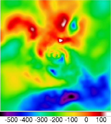
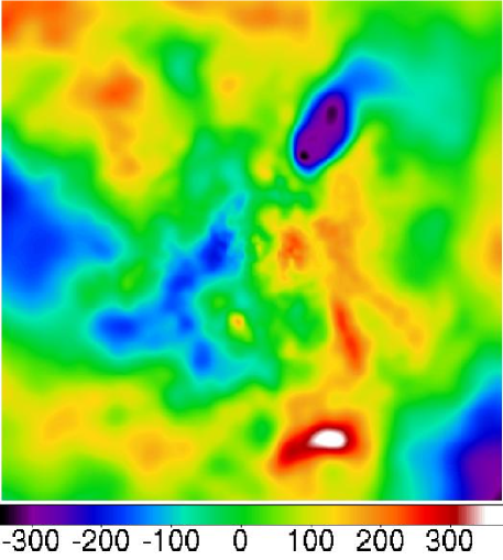
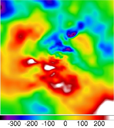
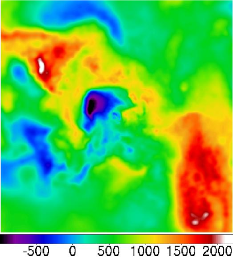
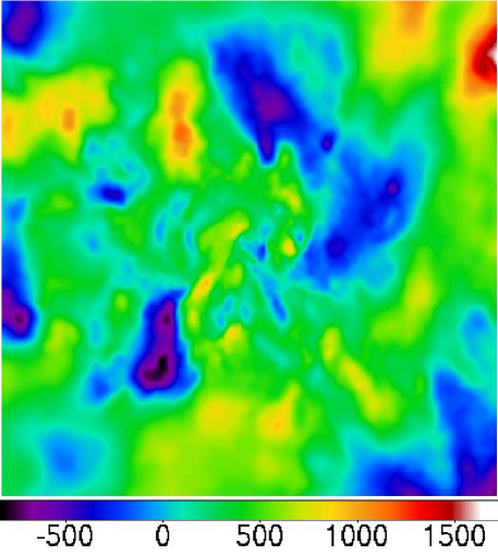
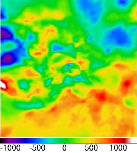
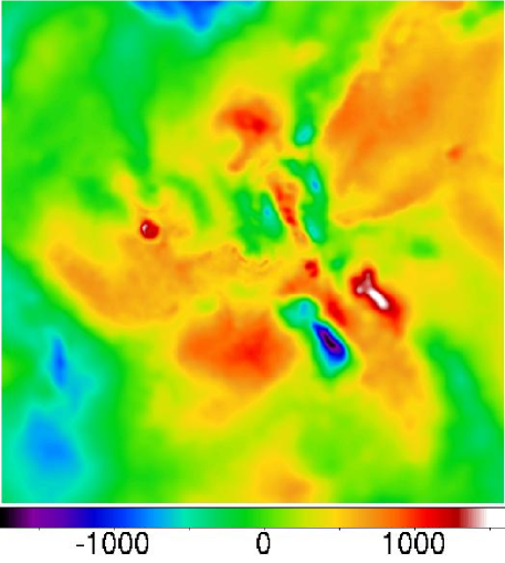
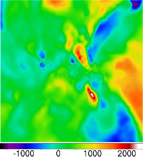
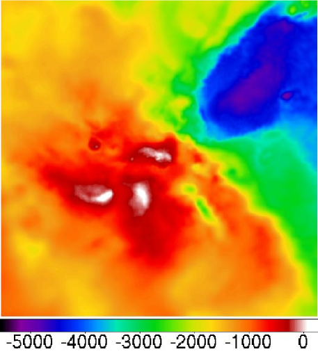
Figure 9: Slices of the velocity field (in km/s) in simulated clusters g6212 (the top panels), g8 (the middle panels) and g72 (the bottom panels). The right column shows x component of velocity, the middle column y component and the left column z component. The slices go through the center of the clusters and have an effective thickness of 3 kpc, corresponding to the size of one cell. The image size is 2$\times$2 Mpc.

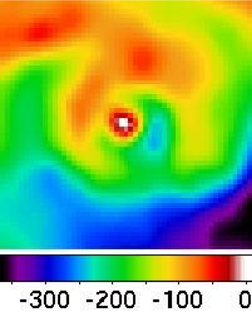
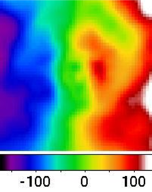
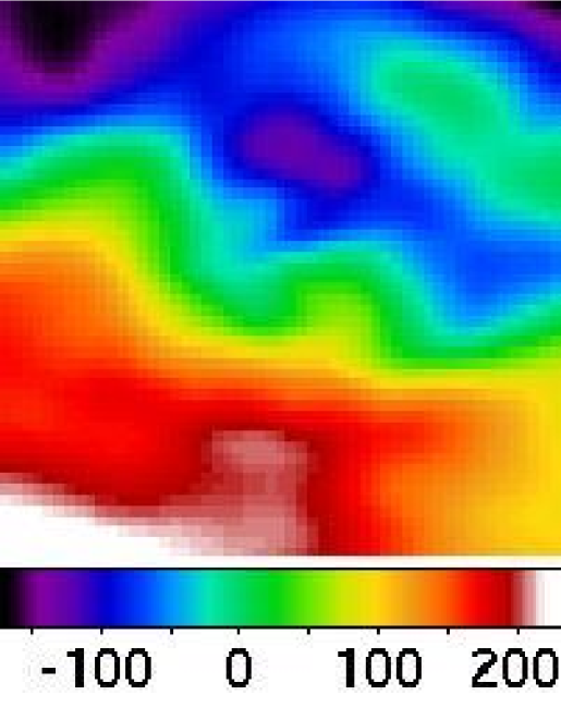
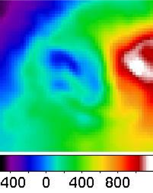
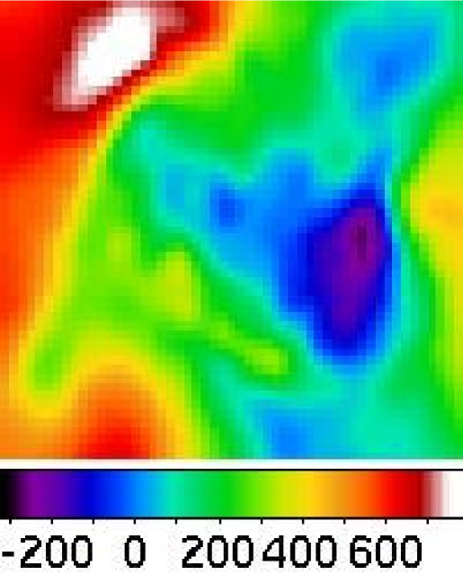
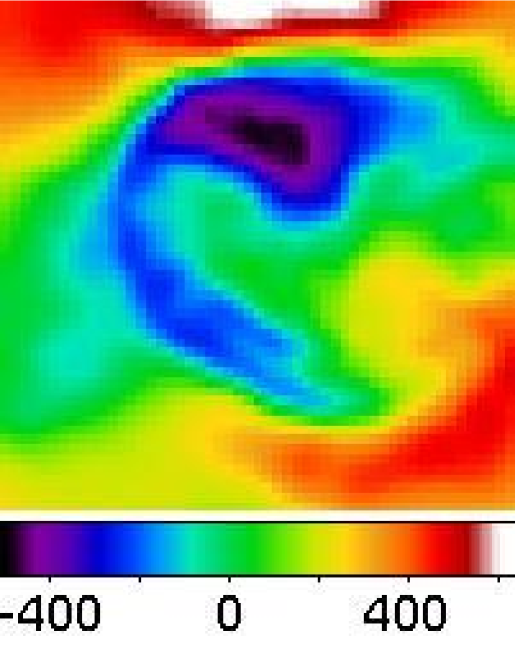
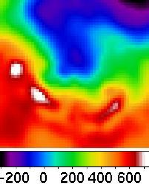
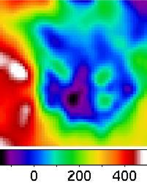
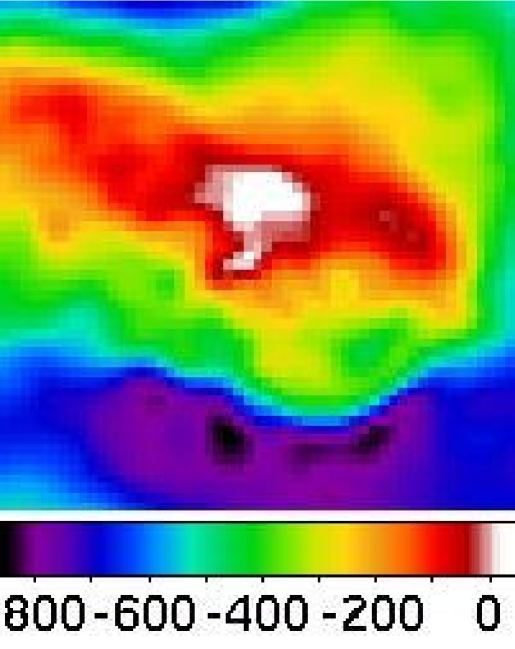
Figure 10: The same as in Fig.9, but for the central part of each cluster. The image size is 100$\times$100 kpc.

From Fig.8, we see that the g6212 cluster is relatively cool with a maximum temperature $\sim$ 2 keV. In such clusters the lines of B-like and C-like iron and lines of lighter elements become strong. But only few of these lines have optical depth large enough for a signficant resonant scattering effect. In Table LABEL:tab:3dline we show the list of lines, which are the strongest in a typical cluster with mean temperature less then 2 keV and have a weight of dipole scattering $\geq 0.5$. The optical depth presented in Table LABEL:tab:3dline was calculated in the line center as

$$\tau=\int\limits_{r_{0}}^{\infty}n_{\rm i}\sigma_{0}{\rm d}r$$ (14)

along an arbitrary chosen radial direction, where the distance from the center $r_{0}\sim 10$ kpc. We avoided integration in the very center of the cluster since the number density in few central cells and their contribution to the optical depth are very high in some of the simulated clusters. We see that for the cluster g6212 the most interesting line is the one at 1.009 keV, which corresponds to the $2s^{2}2p^{2}(^{3}P_{0})-2s^{2}2p3d(^{3}D_{1})$ transition in C-like iron and has a large optical depth and a pure dipole scattering phase function.

In the g8 cluster, the mean temperature is $\sim 15$ keV and the most promising lines for significant resonant scattering are: the K_α line of He-like iron at 6.7 keV and the K_α line of H-like iron at 6.96 keV. The H-like line has two components, $1s(^{2}S_{1/2})-2p(^{1}P_{1/2})$ at 6.95 keV and $1s(^{2}S_{1/2})-2p(^{1}P_{3/2})$ at 6.97 keV. The first component has an oscillator strength 0.135; the total angular momentum is equal to 1/2 both for the ground and excited states, and therefore (Hamilton, 1947) the scattering phase function is isotropic and scattered emission is unpolarized. The second component has an oscillator strength 0.265 and equal weights of dipole and isotropic scattering. The optical depth is $\sim$3.56 for the line at 6.7 keV and $\sim$1.14 for the line at 6.97. Therefore the highest polarization degree in the g8 cluster is expected in the 6.7 keV line of Fe XXV.

The g72 cluster is an example of a merging cluster, as is clearly seen from Fig.8. The mean temperature is similar to the temperature in Perseus, i.e. about 5-6 keV. Therefore the polarization degree was calculated in the 6.7 keV line of He-like iron.

Table 2: Basic properties of simulated clusters g6212, g72 and g8 at $z=0$.

Cluster	$M_{\rm vir}$, $10^{14}$M⊙	$R_{\rm vir}$, Mpc	$T_{\rm min}$, keV	$T_{\rm max}$, keV	$n_{\rm min},~{}{\rm cm}^{-3}$	$n_{\rm max},~{}{\rm cm}^{-3}$
g6212	1.61	1.43	0.2	2.2	1$\cdot 10^{-5}$	0.1
g72	19.63	3.29	0.3	32	7$\cdot 10^{-5}$	0.1
g8	32.70	3.90	3	35	7$\cdot 10^{-5}$	0.2

The velocity field was taken directly from simulations. The slices of velocity components in all three clusters are shown in Fig.9. The slices go through the centers of the clusters and have a thickness of 3 kpc. The motion of a cluster as a whole was compensated for by subtracting the velocity vector corresponding to the central cell. This choice is convenient since it shows the gas velocities relative to the densest (and therefore brightest) part of the cluster, which is responsible for much of the line flux to be scattered in outer regions. To characterize the spread of velocities within the cluster we calculated mass-weighted value of the RMS of the velocity (relative to the velocity of the central cell) over entire volume of a $2\times 2\times 2$ Mpc cube. The RMS values are $\sim 230$ km/s in g6212 cluster, $\sim 1000$ km/s in g8 cluster and $\sim 2400$ km/s in g72. If instead we calculate the RMS relative to the mass-weighted mean velocity the value of RMS decreases to $\sim 800$ km/s for g8 cluster, $\sim 200$ km/s for g6212 cluster and to $\sim 1400$ km/s for g72 cluster. We note here that for radiative transfer calculation the value of the subtracted velocity vector is not important since the polarization signal is only sensitive to the relative velocities of different gas lumps and does not depend on the motion of the cluster as a whole. In Fig.10 velocities of gas motions in the cluster centers are shown. The size of the central region was chosen to be 100$\times$100 kpc. Notations are the same as in Fig.9. The spread of velocities in the centers is lower than at the edges.

In order to see the influence of different gas motions on polarization degree, we made a number of radiative transfer simulations keeping the same density and temperature distributions, but varying the characteristic amplitude of the gas velocities. This was done by introducing a multiplicative factor $f_{v}$ which is used to scale all velocities obtained from the hydrodynamical simulations. In particular $f_{v}=0$ means no motions, $f_{v}=1$ means the velocity field as computed in the simulations, $f_{v}=2$ means doubled velocities compared to hydro simulations, etc. The second parameter characterizing the radiative transfer simulation is the level of micro-turbulence, parametrized via the effective Mach number $M$ (see equations 5 and 6). As discussed above, increasing $M$ causes the optical depth to decrease, leading to the decrease of the polarization signal. Thus the pair of parameters $(f_{v},M)$ completely specifies the scaling of the velocity field in a given radiative transfer run, compared to the original hydrodynamical simulations. In our simulations the values of $f_{\rm v}$ and $M$ are treated as independent parameters, since our goal is to examine separately the impact of the large scale motions and the micro-turbulence on scattering and polarization. Strictly speaking, a more self-consistent approach would be to relate $M$ and the spread of velocities on larger scales, resolved by the simulation, by assuming e.g. Kolmogorov scaling in a turbulent cascade.

The resolution of the SPH simulations used here is not fully sufficient to resolve small scale motions of the ICM. Typical resolved scales vary from few tens kpc in the center to few hundred kpc at the outskirts of simulated clusters. Our approach of ”hiding” unresolved ICM motions as a micro-turbulence (i.e. as line broadening) is valid if the mean free path of the photons is larger than the resolved spatial scales. We tested this approximation for radial distances $\sim$300 kpc from the center and found that this criterion is safely satisfied. We further address this issue elsewhere (Zhuravleva et al., in preparation).

Table 3: Oscillator strengths and optical depths of the strongest X-ray lines with the weight of dipole scattering $\geq$0.5 in the simulated clusters g6212, g72 and g8.

Cluster	Ion	$E$, keV	$f$	$w_{2}$	$\tau$, ($f=0,M=0$)	$\tau$, ($f=1,M=0$)	$\tau$, ($f=0,M=0.25$)	$\tau$, ($f=1,M=0.25$)
g6212	Fe XXV	6.7	0.78	1	2.45	2.02	1.01	0.96
	Si XIII	1.86	0.75	1	1.78	1.47	0.96	0.88
	Fe XXII	1.0534	0.675	0.5	2.86	2.27	1.17	1.1
	Fe XXI	1.009	1.4	1	2.8	2.1	1.16	1.04
g72	Fe XXV	6.7	0.78	1	3.19	0.73	1.32	0.51
g8	Fe XXV	6.7	0.78	1	3.56	1.83	1.47	1.11
	Fe XXVI	6.97	0.265	0.5	1.14	0.52	0.47	0.34

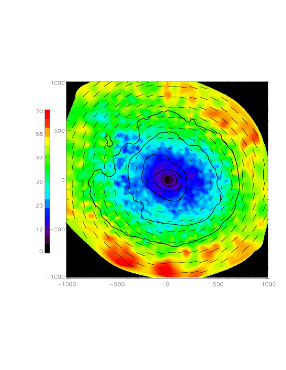
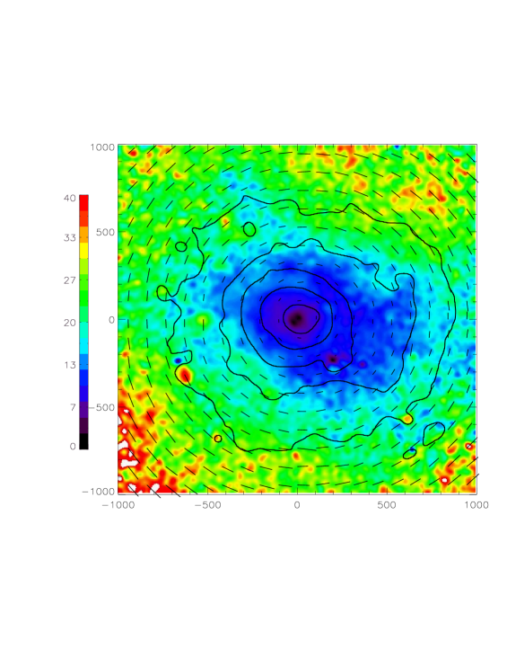
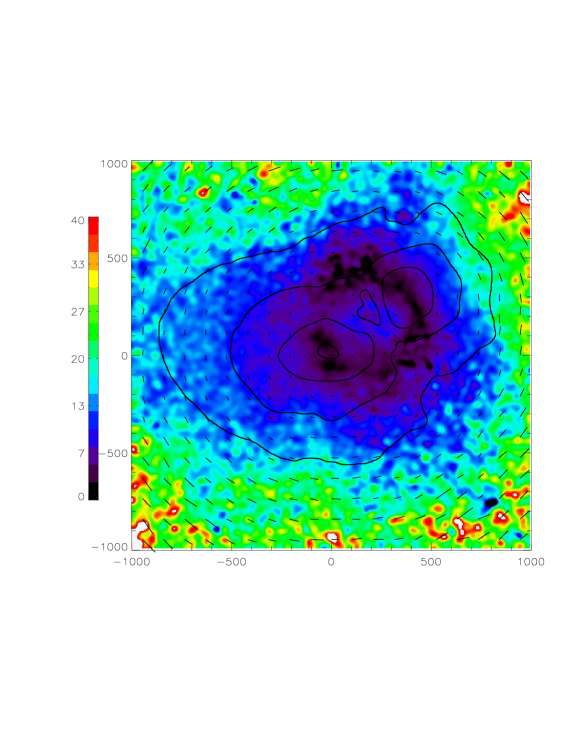
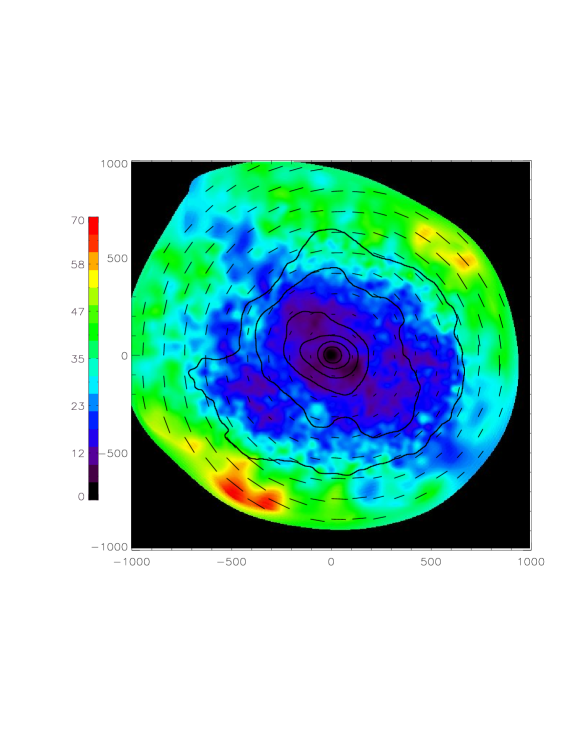
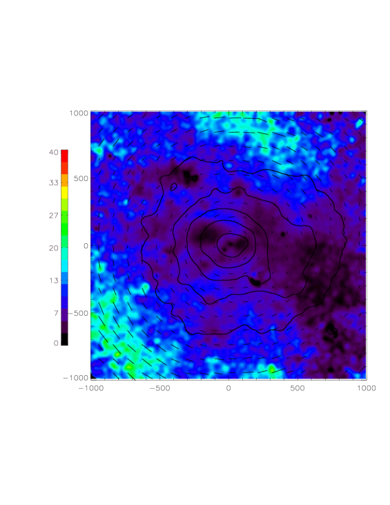
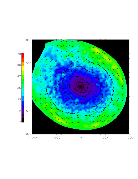
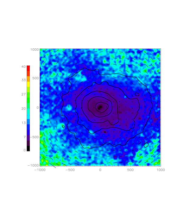
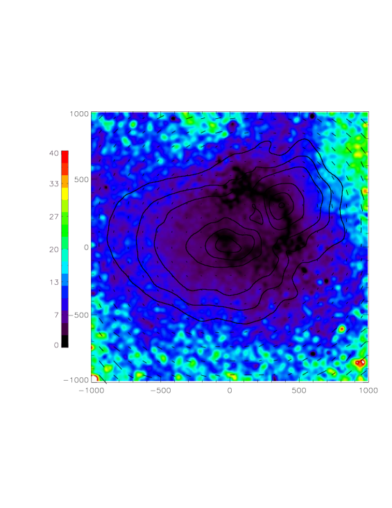
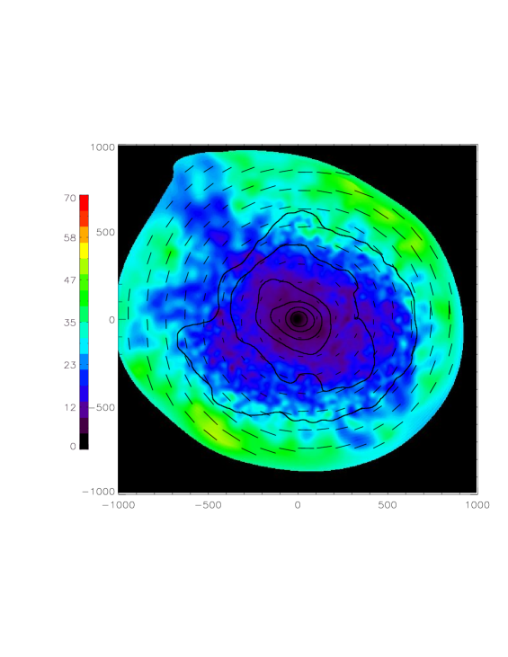
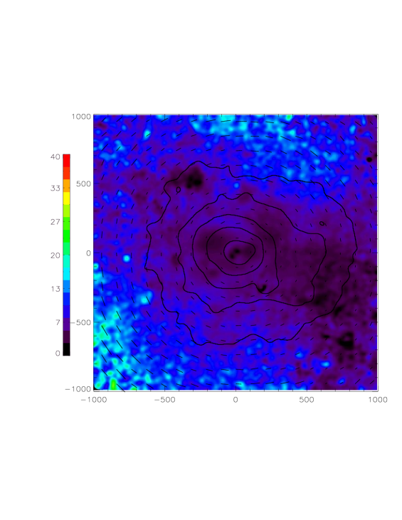
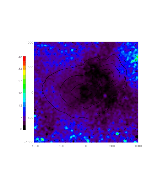
Figure 11: Polarization degree in simulated clusters g6212 (the left panels), g8 (the middle panels) and g72 (the right panels). For the g8 and g72 clusters, the polarization degree was calculated in the K_α line of Fe XXV at 6.7 keV and for the g6212 cluster calculations were done in Fe XXI line at 1.009 keV. The polarization degree was evaluated as $P=\sqrt{Q^{2}+U^{2}}/I$, the value of which is shown in colorbar in percent. $I$ is the total intensity, including scattered and direct emission. The colors in the images show polarization degree, the short dashed lines show the orientation of the electric vector. The contours (factor of 4 steps in intensity) of the X-ray surface brightness in the chosen line are superposed. The size of each picture is 2$\times$2 Mpc. The top three pictures correspond to the case of no motion ($f_{\rm v}=0$, $M=0$). The second raw of pictures shows the case of simulated gas motions ($f_{\rm v}=1$, $M=0$). The third raw shows the polarization when there are only turbulent motions with Mach number $M=0.25$ and the bottom three pictures demonstrate the case of simulated gas motions and turbulent motions ($f_{\rm v}=1$, $M=0.25$). All results were adaptively smoothed.

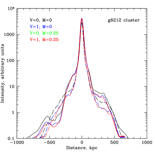
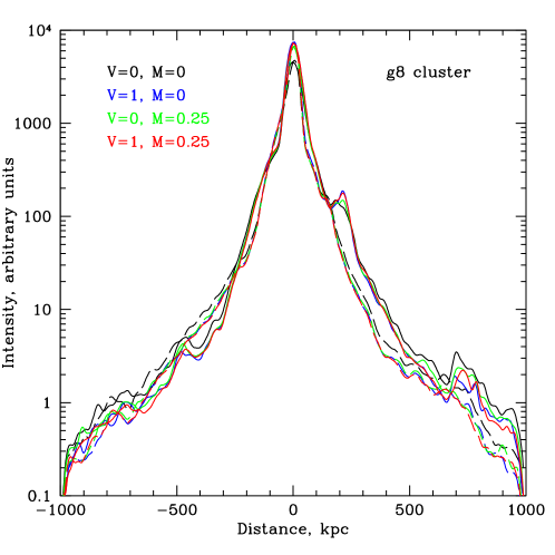
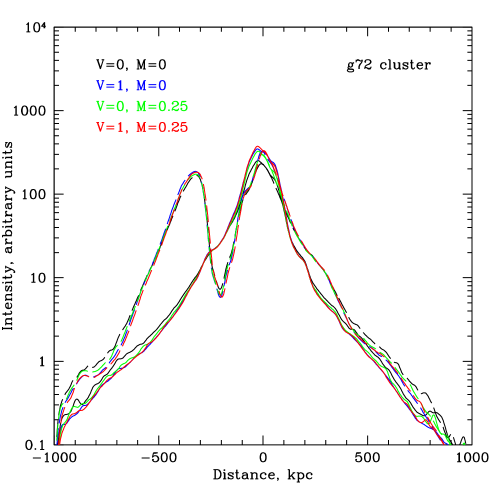
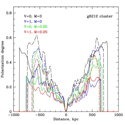
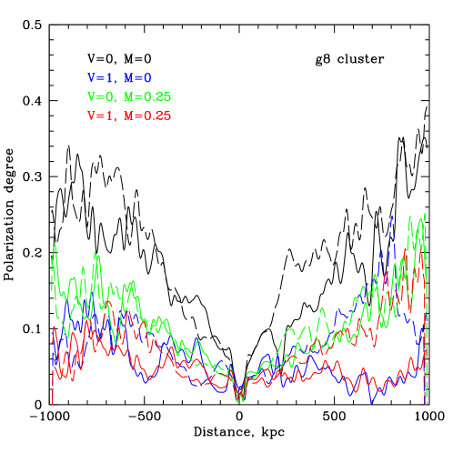
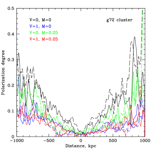
Figure 12: Radial slices of the surface brightness and the polarization degree for the g6212 cluster (right column), g8 cluster (middle column) and g72 cluster (left column), illustrating radial variations of these parameters for two position angles. Colors correspond to different combinations of the velocity factor $f_{v}$ and the Mach number $M$, labels are shown in the top left corner. Solid curves show slices going from the top left conner to the bottom right conner of images shown in Fig. 11. The dashed curves show slices going from the top right conner to the left bottom.

In Fig.11 and Fig.12 we show the results of radiative transfer calculations for the three clusters discussed above. Calculations are done for various combinations of the parameters $f_{v}$ and $M$, namely ($f_{\rm v}=0,M=0$), ($f_{\rm v}=1,M=0$), ($f_{\rm v}=0,M=0.25$) and ($f_{\rm v}=1,M=0.25$). For the g6212 cluster, calculations are done for the L-shell line of C-like iron at 1.009 keV as discussed above. For the g8 and g72 clusters we analyze the Fe XXV line at 6.7 with optical depth $\sim$3.6 and $\sim$3.2 respectively. For g8 and g6212 clusters we consider multiple scattering by setting the minimum photon weight to $10^{-8}$ (see section 3). For g72 cluster (merger of two subclusters) we take into account only the first scattering. Under the conditions characteristic for galaxy clusters, accounting of multiple scattering does not have strong impact on the degree of polarization.

As expected in the very center of each cluster the radiation field is almost isotropic and the polarization degree is accordingly very low, increasing to the cluster edges.

We note here that apart from the real increase of the polarization signal towards the cluster outskirts, there are two spurious effects which lead to the increase of the polarization degree close to the edges of the simulated cube. i) The first effect is similar to the effect of finite $r_{\rm max}$ considered in the previous section (see Fig. 3): near the edges of the simulated volume, the radiation field is strongly anisotropic and the role of 90^∘scattering is enhanced where the line of sight is tangential to the boundary of the simulated volume. From the experiments with spherically symmetric models and the cubes of different sizes we concluded that it is safe to use the data at the projected distance approximately half of $R_{\rm max}$. For our cubes which are $\sim$2 Mpc on a side, this means that the results within a 500 kpc circle (radius) are robust. ii) The second effect is caused by limited photon statistics in the regions close to the image edges, generated by our Monte-Carlo code. The code is optimized to produce the smallest statistical uncertainties in the more central regions of simulated clusters. With only few simulated photons in the outskirts of a cluster, the derived degree of polarization can be spuriously very high - e.g. it is $\equiv 1$ if there is only one photon in a pixel. We suppress this effect by making sufficiently large smoothing windows: $I$, $Q$ and $U$ images are first smoothed and the polarization degree is calculated using smoothed images. The net result of these two effects is that outside the central 0.5 Mpc (radius) circle the estimated degree of polarization is less robust than in the inner region. As discussed below the outskirts of clusters are not a very promising target for measurements of the polarization.

In the g6212 cluster, the degree of polarization reaches 30-35% within a projected distance of $\sim 500$ kpc from the cluster center for the case ($f_{\rm v}=0$, $M=0$). Adding bulk velocity from simulations and no microturbulence ($f_{\rm v}=1$, $M=0$) causes a decrease of the optical depth from almost 3 to $\sim$2, while the degree of polarization decreases to $\sim$20-25%. If only turbulent motions are included ($f_{\rm v}=0$, $M=0.25$), then the optical depth drops to $\sim$ 1.16. The maximum polarization degree in this case is about 25$\%$ as shown in Fig.11. The combination of bulk velocities and micro-turbulence ($f_{\rm v}=1$, $M=0.25$) further decreases the polarization signal and, according to our simulations, the maximum is about 15$\%$ (Fig.11, the bottom left panel).

In the g8 cluster, the polarization degree does not exceed 27$\%$ for the case ($f_{\rm v}=0$, $M=0$) within 500 kpc from the cluster center. As in the previous example the gas motions affect the optical depth, diminishing it and leading to the decrease of the degree of polarization: for $f_{v}=1$ the degree of polarization $P$ is less then 10$\%$ (Fig.11).

For the g72 cluster the situation is similar: when there are no motions, polarization reaches $\sim$20$\%$ at a distance $r=500$ kpc from the cluster center and gas motions reduce the polarization to 7$\%$.

The simulations discussed above are also illustrated in Fig.12, where radial slices of the surface brigtness and the polarization degree are shown for the same set of simulations as in Fig.11.

Results for various other combinations of $f_{\rm v}$ and $M$ for the g6212 cluster are shown on Fig.13. Here, we show the projected polarization degree as we did in the spherically-symmetric case. The left panel shows profiles of polarization for velocity factors $f_{\rm v}=$0, 1, 2 and 5 and the right panel for Mach numbers $M=$0, 0.25, 0.35 and 0.45. This results are in a good agreement with our predictions discussed above.

In our 3D simulations we assume a flat iron abundance profile of 0.79 solar. Any changes in the abundance profile will have an impact on the optical depth in lines and hence can affect the strength of the line scattering and the degree of polarization. Obviously, an overall decrease of the abundance will cause the decrease of the polarization signal.

An impact of a peaked abundance profile on the polarization signal is less obvious. Peaked abundance profiles are often observed in cool core clusters. The abundances vary from $\sim 0.3$ in the outer regions to $\sim 1.2$ at the center (e.g. Pratt et al., 2007). To test this case we consider an averaged metallicity profile for cool core clusters parametrized by De Grandi et al. (2004) as a function of $r/r_{200}$, where $r_{200}$ is the radius corresponding to the mean overdensity of 200$\times$ the critical density of the Universe. We used the mean temperature of simulated clusters to evaluate $r_{200}$ and assumed that the metallicity is linearly decreasing with radius for $r<0.15r_{200}$ and is constant at larger radii. Rescaling the results of De Grandi et al. (2004) to the iron abundance scale of Lodders (2003) ,the final iron abundance changes from 0.85 at the center to 0.44 at large radii. Repeating the radiative transfer calculations we found only a very slight ($\sim$10%) decrease of polarization degree (compared to the flat profile case) in the outer regions where the abundance has changed by almost a factor of 2: from 0.79 (flat profile) to 0.44 (peaked profile). The reason for this stability is as follows: polarized flux from outer parts of a cluster is largely due to the scattered line photons coming from the central bright region. This flux is obviously proportional to the product of the flux from the central region $F_{\rm central}$ and the optical depth of the outer region $\tau_{\rm outer}$. The optical depth in turn is proportional to the abundance $Z_{\rm outer}$. The polarization signal is diluted by the flux of ”locally” generated unpolarized line photons $F_{\rm outer}$, which is also proportional to the abundance in the outer regions and to the product of the flux from the central region and the optical depth of the outer region, i.e. $\displaystyle P\approx\frac{a\tau_{\rm outer}F_{\rm central}}{b\tau_{\rm outer}F_{\rm central}+F_{\rm outer}}$, where $a$ and $b$ are some constants, which depend on the density distribution. Since both numerator and denominator scales linearly with the abundance $Z_{\rm outer}$ this dependence partly cancels out. In other words in the outer regions of clusters in the limit of low abundances the degree of the polarization is approximately proportional to the expression $\displaystyle\frac{\tau_{\rm outer}F_{\rm central}}{F_{\rm outer}}\propto\frac{Z_{\rm outer}F_{\rm central}}{Z_{\rm outer}}\approx F_{\rm central}$ . Thus these two effects partly cancel each other leading to a relatively weak dependence of the degree of polarization on the abundance. In other words, the increase of the flux coming from the central region has larger impact on the polarization degree than the changes in abundance in outer regions (see also Sazonov, Churazov & Sunyaev, 2002, for the limiting case of a strong central source, when a dilution by locally produced line photons is not important).

Note, that these calculations assume that the line photons can be separated from the continuum, i.e. the energy resolution of the polarimeter is very high (see Section 6 for the discussion of the impact of limited energy resolution on the polarization signal).

5.1 Major merger

A particularly interesting case is when the polarization degree increases due to the anisotropy caused by gas motions. This can happen, for example, when gas blobs are moving in the cluster center or when two galaxy clusters are merging. The well-known example of merging clusters is the Bullet cluster in which gas motions reach velocities up to 4500 km/s. Even if the radiation field is originaly isotropic (e.g. in the very center of the galaxy cluster) the dependence of the scattering cross section on energy (see section 1) will produce anisotropy and polarization in the scattered radiation.

Figure 13: Radial profiles of polarization degree in the Fe XXI iron line at 1.009 keV for the simulated cluster g6212 for different values of velocity factors and Mach numbers. The left panel: the solid line is for ($f_{\rm v}$=0, $M$=0), the short dashed line for ($f_{\rm v}$=1, $M$=0), the long dashed line is for ($f_{\rm v}$=2, $M$=0) and the dot-dashed line is for ($f_{\rm v}$=5, $M$=0). The corresponding RMS values of the gas velocities $V_{{\rm rms}}$ in km/s are shown in the upper left corner. The right panel: the solid line is for ($f_{\rm v}=0$, $M=0$), the short dashed line for ($f_{\rm v}=0$, $M=0.25$), the long dashed line for ($f_{\rm v}=0$, $M=0.35$) and the dot-dashed line for ($f_{\rm v}=0$, $M=0.45$).

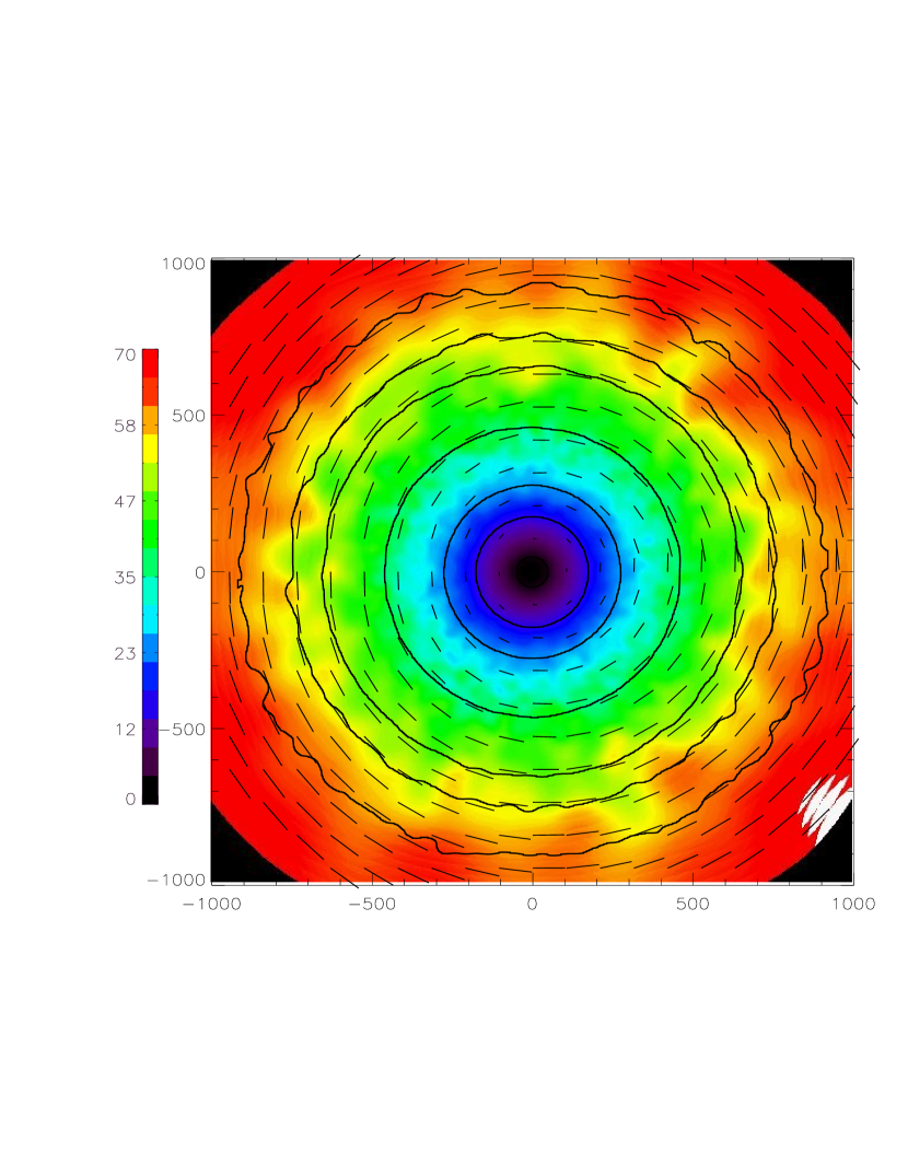
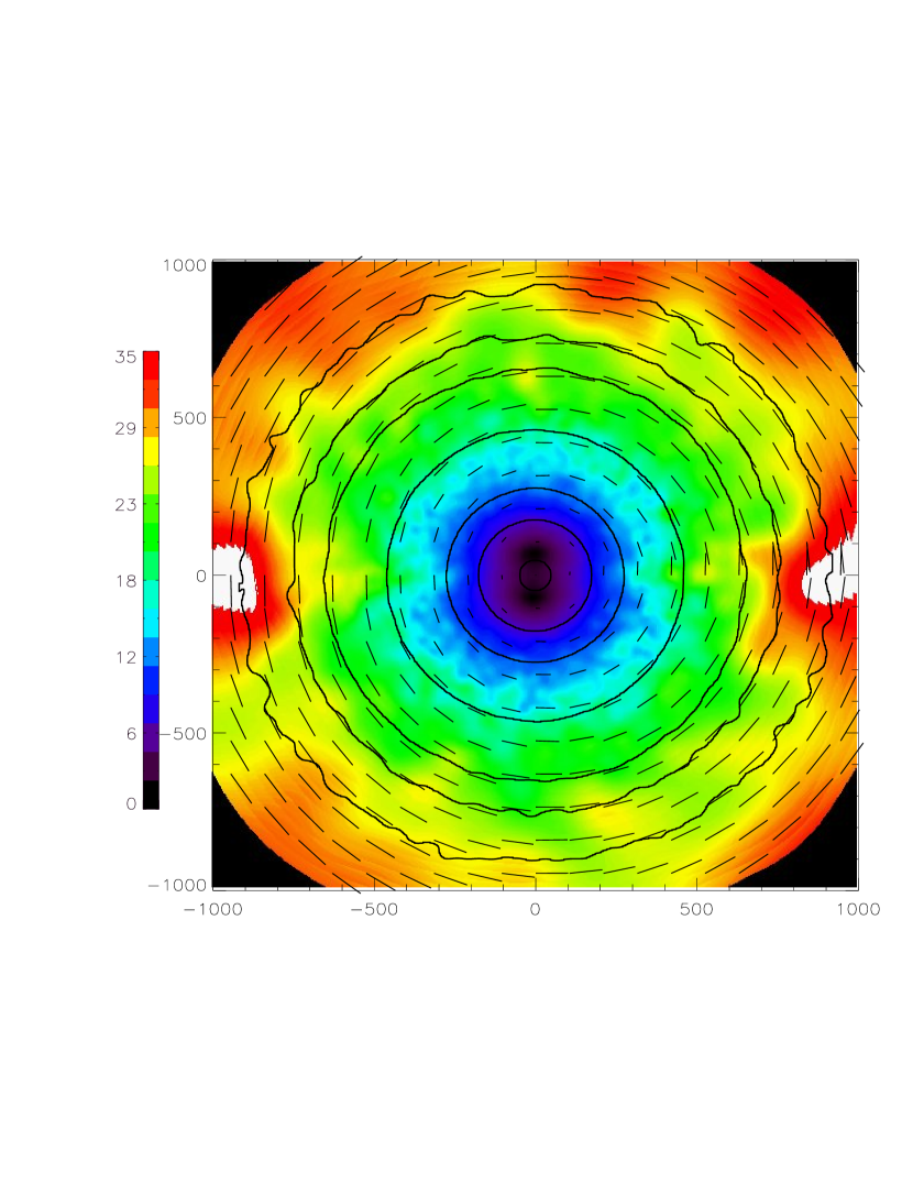
Figure 14: Polarization degree in a spherically-symmetric $\beta-$model galaxy cluster with $n_{0}=10^{-2}$ cm^-3, $r_{\rm c}=100$ kpc, $\beta=1$. Temperature is constant $T=5$ keV and iron abundance is 0.79 solar. Calculations were done for the He-like iron line at 6.7 keV. The polarization degree was evaluated as $P=\sqrt{Q^{2}+U^{2}}/I$, the value of which is shown in the colorbar in percent. $I$ is intensity of both direct and scattered emission.The colors in the images show the polarization degree, the short dashed lines show the orientation of the electric vector. The contours of the X-ray surface brightness in the chosen line are superposed. The size of each picture is 2$\times$2 Mpc. On the left panel are shown results when the gas is motionless. On the right panel is shown the case when two parts of the cluster are moving towards each other with velocities 500 km/s and -500 km/s respectively. In this case the asymmetry in the radiation field appears in the very center of the galaxy cluster and the polarization degree reaches about 2$\%$.

To model the polarization from a major merger, we consider an illustrative example: two halves of galaxy cluster are moving towards each other with velocities $\pm$500 km/s. In such a situation, an anisotropy in the scattering cross section (see eq. 1) can produce polarized radiation even in the cluster center. We used a simple spherically-symmetric $\beta-$model for the density distribution $n_{0}=10^{-2}$ cm^-3 with $r_{\rm c}=100$ kpc, $\beta=1$. The temperature of cluster is constant $T=5$ keV and the iron abundance is 0.79 solar. Calculations were done for the He-like iron line at 6.7 keV. To show the sensitivity of polarization to the tangential component of gas motions, we assume that only the y-component of velocity is non-zero, while the viewing vector is along the z-axis (see, e.g. Fig.2). Fig.14 shows the results of our calculations. We see that in the case of such motions, the polarization in the center increases from 0$\%$ to 2$\%$.

6 Discussion

Our results show that, owing to the asymmetry in the radiation field, the polarization for the brightest X-ray lines from galaxy clusters can reach values as high as 30$\%$. In addition, we have shown that the polarization degree is sensitive to gas motions. Therefore, polarization measurements provide a method to estimate velocities of gas motions in the direction perpendicular to the line of sight.

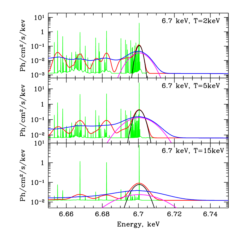
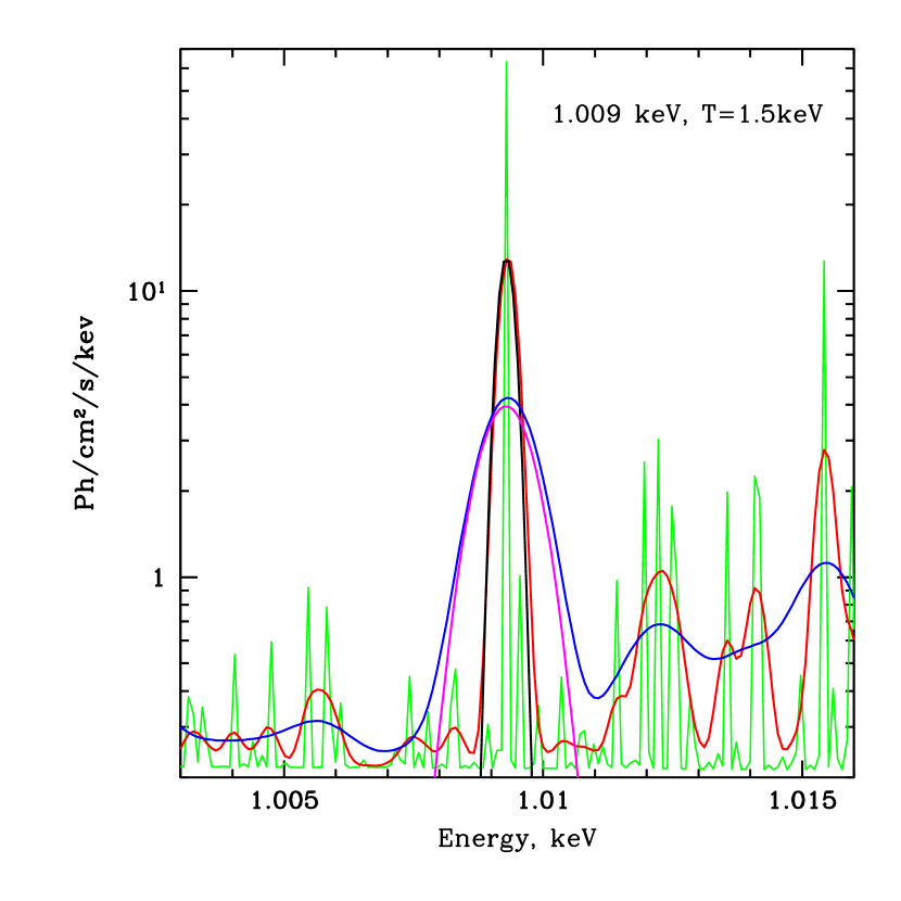
Figure 15: Top panel: changes of the polarization degree as a function of the instrument energy resolution. On the upper panels results are shown when only thermal broadening of lines is considered. The cases when turbulent broadening is included are shown on the lower panels. The lines in the left panel show the ratio of the resonant line flux (6.7 keV permitted line) to the total (continuum plus all lines) flux within an energy interval of a given width centered at the line energy. The solid, long dashed and short dashed lines correspond to plasma with the temperature of 2, 5 and 15 keV respectively. In the right panel similar curves are shown for the bright low energy lines: Fe XXI line at 1.009 keV (solid line), Fe XXIII line at 1.129 keV (short dashed line) and Fe XXII line at 1.053 keV (long dashed line) for the plasma with the the temperature 1.5 keV. The iron abundance is assumed to be 0.79 solar. Only the flux in the line is assumed to be polarized.
Bottom panel: model spectra of the hot optically thin plasma with different temperatures.
Color coding:
Green - spectrum with no line broadening (apec model in XSPEC).
Red - spectrum with pure thermal line broadening (bapec model of XSPEC).
Black - the Gaussian profile of the main line for pure thermal broadening.
Blue - spectrum with thermal and turbulent line broadening (bapec model of XSPEC). Turbulent velocities are set to $V_{{\rm turb}}=0.25c_{\rm s}$.
Magenta - the Gaussian profile of the main line, accounting for the thermal and turbulent broadening.
The left panel: model spectrum of cluster with temperature 2, 5 and 15 keV (the top, middle and bottom panels respectively). The main line is the Fe XXV line of He-like iron at 6.7 keV. The right panel: model spectrum for temperature 1.5 keV. The main line is the Fe XXI line at 1.009 keV.

One of the limiting factors which affects the expected degree of polarization is the contamination of the polarized emission in the resonant line by the unpolarized emission of the continuum emission of the ICM and neighboring lines. This factor critically depends on the energy resolution $\Delta E$ of the polarimeter. If we assume that only the emission in a given line is polarized, the measurable polarization will differ from the idealized case by a factor $f=F_{\rm line}/F_{\rm tot}$, where $F_{\rm line}$ is the flux in the resonant line and $F_{\rm tot}$ is the total flux measured by the detector in an energy band $\Delta E$ centered on the resonant line energy. In Fig.15 we plot this factor as a function of the width of the energy window (detector energy resolution) for different theoretical spectra for the model clusters discussed above assuming only thermal line broadening and both thermal and turbulent broadening. One can see that the contamination of the 6.7 keV line flux by the unpolarized flux is very minor for an energy resolution better than $\leq$ 10 eV. For the energy resolution of 100 eV the fraction of contaminating unpolarized flux is of order 30-60% depending on the plasma temperature. This line is most prominent in clusters with temperatures $\sim$ 3-6 keV as the line flux at such temperatures is the largest and neighbouring lines are not as strong as in a case of $\sim$2 keV plasmas (see the bottom left panel on Fig.15). For lines with energies $\sim$1 keV even better energy resolution is needed since in the spectrum there is a forest of low energy lines and the contamination from these lines dramatically decreases the flux of polarized emission (see the bottom right panel on Fig.15).

Another effect which also depends on the energy resolution of the polarimeter is the contamination of line flux by the contribution of the cosmic X-ray background (CXB) which starts to dominate at some distance from the galaxy cluster center. Assuming that the CXB is not resolved into individual sources by the polarimeter the contribution of the CXB starts to be the dominant source of contamination at a distance from the cluster center where the surface brightness of the cluster continuum emission matches the CXB surface brightness (at the line energy). As an illustrative example we use the results of simulations for the g6212 cluster in the Fe XXI line at 1.0092 keV, setting $f_{v}=0$ and $M=0$, and similarly for the g8 cluster in the Fe XXV line at 6.7 keV and for the g72 cluster in the same line. All clusters are placed at a distance of 100 Mpc and the energy resolution of the instrument is set to 10 eV. Using the CXB intensity from Gruber et al. (1999) (see also Churazov et al., 2007) we calculated the expected degree of polarization (Fig.16) including a CXB “contamination” flux $I_{CXB}\times\Delta E$. Accounting for the finite energy resolution and contamination by the ICM emission affects the polarization signal from any region of a cluster, while the CXB contribution (for an instrument with a modest energy resolution) effectively overwhelms the polarization signal in the cluster outskirts. In Fig.16 we show results for the g6212, g8 and g72 clusters, where the limiting factors discussed above are taken into account. According to Fig.15 the limiting factors due to the ICM are 0.6, 0.85 and 0.95 for g6212, g8 and g72 clusters if we assume an energy resolution of 10 eV. First we see that inclusion of the CXB reduces the very high polarization degree in the outer parts of clusters. Second, the polarization degree is reduced everywhere by “contamination” from unpolarized radiation. Within the central region ($r\approx$500 kpc), the polarization degree decreases from 30-35$\%$ to 20$\%$ in the g6212 cluster, from 27$\%$ to 20$\%$ in the g8 cluster. For the g72 cluster, the degree of polarization does not change significantly, since the contamination by the unpolarized radiation is small in this case.

It is also interesting to note, that when gas motions with velocities up to a few 1000 km/s exhibit, the Doppler shifts corresponding to such velocities are comparable or larger than some doublet separations (see e.g. Fig.15). And flux from one line can be scattered in another neighbouring line. This can easily happen, for example, in doublet with the components at 6.97 keV and 6.93 keV.

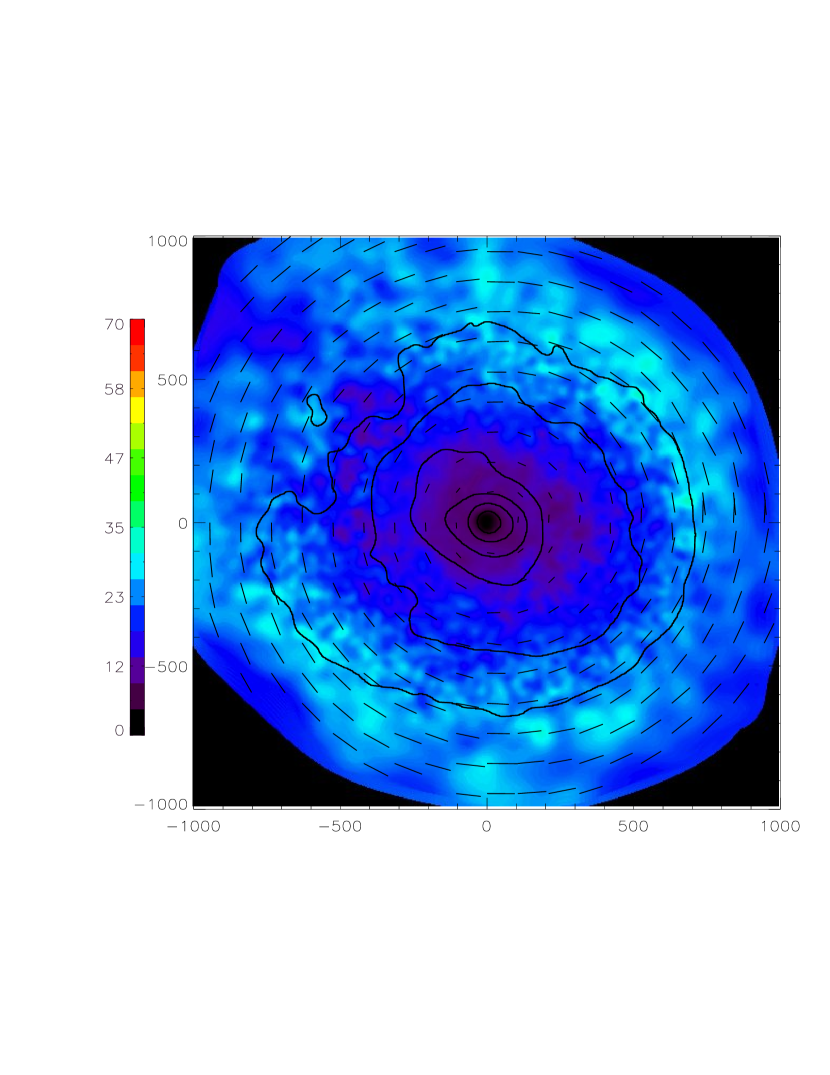
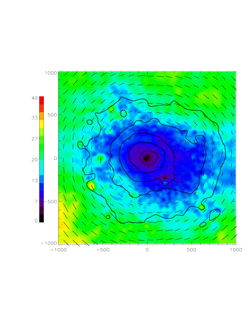
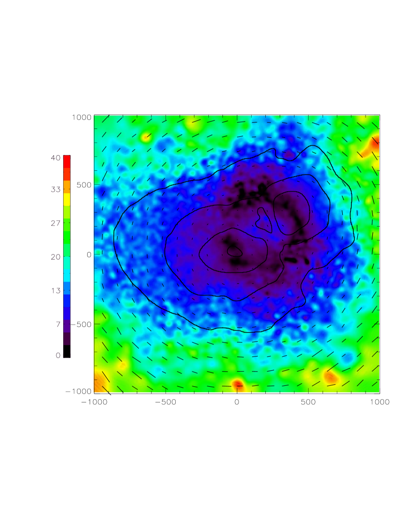
Figure 16: Polarization degree for simulated clusters g6212 (the top left panel), g8 (the top right panel) in the lines of Fe XXI at 1.0092 keV and Fe XXV at 6.7 keV, respectively, and for the g72 cluster (the middle bottom panel) in the 6.7 keV line. The polarization degree was evaluated as $P=\sqrt{Q^{2}+U^{2}}/I$, the value of which is shown in colorbar in percent. $I$ in a total intensity, i.e. intensity of scattered and direct emission. The colors in the images show polarization degree, the short dashed lines show the orientation of the electric vector. The contours of the X-ray surface brightness (factor of 4 steps) in the chosen line are superposed. The size of each picture is 2$\times$2 Mpc. The gas is motionless ($f_{\rm v}=0$, $M=0$). The CXB radiation is included and the energy resolution is 0.01 keV. Also the decrease of polarization degree due to the continuum and neighboring non-polarized lines is taken into account. According to Fig.15 the limiting factor for the 1.0092 keV line in g6212 cluster is 0.6, for the 6.7 keV line in g8 cluster is 0.85 and for the same line in the g72 cluster is 0.95.

7 Requirements for future X-ray polarimeters

Galaxy clusters are promising, but challenging targets for future polarimetric observations which pose requirements to essentially all basic characteristics of the telescopes, such as angular and energy resolutions, effective area and the size of the field of view. (i) First of all, in order to detect polarization in lines polarimeters should have good energy resolution to avoid contamination of the polarized line flux by the unpolarized continuum and nearby lines (Fig.15). (ii) An angular resolution has to be better than an arcminute even for nearby clusters. Indeed, the polarization largely vanishes when integrated over the whole cluster. For instance, the polarization of the 6.7 keV line flux, integrated over the whole cluster, is 1.2%, 0.55% and 1.2% for the g6212, g8 and g72 clusters respectively. As is clear from e.g. Fig.11 the polarization direction is predominantly perpendicular to the radius and the polarization degree varies with radius (see Fig.3). Therefore, to get most significant detection it is necessary to resolve individual wedges and to combine the polarization signal by aligning the reference frame, used for the calculations of Stokes parameters, with the radial direction. For nearby clusters (e.g. Perseus) this requires an arcminute angular resolution. (iii) Since the polarization is small in the central bright part of the cluster (e.g. Fig.3) the instrument should have sufficiently large effective area to collect enough photons from the cluster outskirts. (iv) For the same reason a large Field-of-View is important for collecting a large number of photons from the brightest nearby clusters like Perseus.

Currently, several polarimeters based on the photoelectric effect are actively discussed (see e.g. Costa et al. (2001); Muleri et al. (2009); Bellazzini et al. (2007); Jahoda et al. (2007); Soffitta et al. (2001)). These are basically gas detectors with fine 2-D position resolution to exploit the photoelectric effect. When a photon is absorbed in the gas, a photoelectron is emitted preferentially along the direction of polarization. As the photoelectron propagates its path is traced by the generated electron-ion pairs, which are amplified by a Gas Electron Multiplier (GEM) and are collected by a pixelized detector. Hence the detector sees the projection of the track of the photoelectron.

One of the polarimeters based on photoelectric effect is GEMS (Gravity and Extreme Magnetism SMEX) of the NASA SMEX program. This polarimeter will provide polarization measurements in the standard 2-10 keV band with energy resolution $\Delta E/E=0.2$, a modulation factor $\mu=$0.55 and an effective area of $\sim$600 cm² at 6 keV.

Another proposed instrument is EXP (Efficient X-ray Photoelectric Polarimeter) polarimeter on-board HXMT (Hard X-ray Modulation Telescope). This telescope has a large field of view (FoV) $22^{\prime}\times 22^{\prime}$, mirrors effective area $\sim$280 cm² at 6.7 keV and the detector quantum efficiency (QE) of about 3$\%$. The energy resolution is $\Delta E/E=0.2$ at 6.7 keV (Costa et al., 2007; Soffitta et al., 2008).

Polarimeters have been also proposed as focal plane instruments for the International X-ray observatory (IXO) (Costa et al., 2008).

Most important characteristics of discussed polarimeters are summarized in Table LABEL:tab:polar. We also show in this table the characteristics of a hypothetical polarimeter, which would be suitable for the study of polarized emission lines in galaxy clusters. The key difference of this hypothetical polarimeter with the currently discussed GEM polarimeters is the energy resolution of 100 eV and larger efficiency.

Obviously only the brightest clusters have a chance of being detected with the current generation of X-ray polarimeters. Discussed below is the case of the Perseus cluster, which is the brightest cluster in the sky and as such is the most promising target. The degree of polarization in the 6.7 keV resonant line flux is shown in Fig.3. While the surface brightness declines with radius, the degree of polarization is instead steadily increasing with radius. It is possible therefore that the optimal signal-to-noise ratio (S/N) is achieved at some intermediate radius. The expected modulation pattern in a given pixel of the cluster image is proportional to

$$c+\mu pc\cos(2\phi+\phi_{0}),$$ (15)

where $c$ is a number of counts in this pixel, $\mu$ is a modulation factor, $p$ and $\phi_{0}$ are the degree of polarization and the angle of the polarization plane with respect to the reference coordinate system. One can fit the observed modulation pattern with a function

$$x_{1}+x_{2}\cos(2\phi),$$ (16)

where $x_{1}$ and $x_{2}$ are the free parameters. In the above expression we set $\phi_{0}$ to zero, since the polarization plane is perpendicular to the radial direction (in the first approximation) and therefore the angle is known. We assume below that for any pixel of the cluster image the reference system is aligned with the radial direction. This way the Stokes Q and U parameters obtained in individual pixel can be averaged over any region of interest. The final S/N ratio, characterizing the significance of the polarization detection from the region is

$$\left(\frac{S}{N}\right)_{0}=\displaystyle\frac{<x_{2}>}{\sigma_{<x_{2}>}}=\displaystyle\mu\frac{\sum\limits_{i}p_{i}c_{i}}{\sqrt{2\sum\limits_{i}c_{i}}},$$ (17)

where the summation is over all pixels in the region. If an unpolarized flux of the continuum and neighbouring lines is contributing to the total flux seen by the detector (see §6) then the S/N ratio will scale as the square root of the line and total fluxes:

$$\frac{S}{N}=\left(\frac{S}{N}\right)_{0}\sqrt{\frac{F_{\rm line}}{F_{\rm tot}}},$$ (18)

where $\left(\frac{S}{N}\right)_{0}$ is the S/N ratio for the pure line flux.

Table 4: The main characteristics of HXMT(Costa et al., 2007; Soffitta et al., 2008), IXO(Costa et al., 2008), GEMS(Jahoda et al., 2007) and hypothetical polarimeters.

	HXMT	IXO	GEMS	Hypothetical polarimeter
Mirrors Effective Area @ 6.7 keV	280 cm2	5600 cm2	600 cm2	1000 cm2
Field of View	$22^{\prime}\times 22^{\prime}$	$2.6^{\prime}\times 2.6^{\prime}$	$14^{\prime}$	$20^{\prime}\times 20^{\prime}$
Angular Resolution	$1^{\prime}$	$5^{\prime\prime}$	$1.8^{\prime}$[HPD]	$1^{\prime}$
Energy Resolution	$\Delta E/E=0.2$	0.2	0.2	100 eV
Modulation Factor @ 6 keV $\mu$	0.65	0.65	0.55	0.65
Detector Quantum Efficiency @ 6 keV	0.023	0.023	0.1	0.5

The S/N ratio for the 6.7 keV line in Perseus is shown in Fig.17. For this plot we assume that a hypothetical polarimeter with the characteristics given in Table LABEL:tab:polar is observing the cluster for 1 Megasecond. In the bottom panel the S/N ratio was calculated for $1^{\prime}\times 1^{\prime}$ square regions located at a given distance from the center of the Perseus cluster. The solid line is calculated assuming that only 6.7 keV line photons are detected (i.e. $\left(\frac{S}{N}\right)_{0}$), while the dashed line shows the S/N ratio for an instrument with the energy resolution of 100 eV (and therefore the continuum and nearby lines decrease the degree of polarization). In the top panel of Fig.17 the S/N ratio is calculated for a set of annuli with inner and outer radii $R_{1}=R$ and $R_{2}=1.5\times R$ and plotted as a function of $R$. In our model of the Perseus cluster its surface brightness in the outer regions is described by a $\beta$ model with $\beta=0.5$. Thus for large radii the surface brightness declines as $1/R^{2}$. If the solid angle of the region scales as $R^{2}$ (as is the case for the annuli used in the top panel of Fig.17) these two factors cancel each other and the S/N ratio as a function of radius simply follows the variations in the degree of polarization with radius (see Fig.3). The solid line in the top panel of Fig.17 again corresponds to the line photons only, while the dashed line assumes 100 eV energy resolution. Setting the energy resolution to 1 keV (realistic number for a gas detector) would decrease the S/N ratio from $\sim$18 to $\sim$8 in an annulus near 30^′.

The above analysis suggests that for an instrument with a very small FoV (few arcminutes) the optimal S/N ratio will be achieved if a region at a distance of $4^{\prime}-5^{\prime}$ from the center of the Perseus cluster is observed. For a large FoV (few tens of arcminutes) the optimal strategy is to point directly at the center of the cluster and to combine the signal from the cluster outskirts.

Figure 17: Significance of the 6.7 keV line polarization detection in Perseus cluster. For this plot we assume that a hypothetical polarimeter with characteristics listed in Table LABEL:tab:polar is observing the cluster for 1 Megasecond. The solid line shows the detection significance if only line photons are detected, while the dashed line shows the S/N ratio for an instrument with the energy resolution of 100 eV (and therefore the continuum and nearby lines decrease the degree of polarization). Top panel: the S/N ratio is calculated using eq.(17) and eq.(18) for a set of annuli with inner and outer radii $R_{1}=R$ and $R_{2}=1.5\times R$ and plotted as a function of $R$. Bottom panel: the same as in the top panel, but for a $1^{\prime}\times 1^{\prime}$ square region.

Figure 18: Top panel: MDP calculated using eq.19 in the Perseus cluster for a set of annuli with inner and outer radii $R_{1}=R$ and $R_{2}=1.5\times R$ as a function of $R$. The solid curve shows MDP when only flux from the line is included, the dashed curve shows the case when the unpolarized continuum is added. Characteristics of the hypothetical polarimeter were assumed (see Table LABEL:tab:polar)
The bottom panel: statistical uncertainty in $P$ in the Perseus cluster. Notations are the same as in the top panel.

We can recast these results in a form of Minimum Detectable Polarization (MDP) in the line at the 90$\%$ confidence level (S/N=2.6). From eq.18 we get

$${\rm MDP}_{\rm line}=\frac{2.6}{\mu}\sqrt{\frac{2}{\sum\limits_{i}c_{i}}}\frac{F_{\rm tot}}{F_{\rm line}}={\rm MPD}_{0}\sqrt{\frac{F_{\rm tot}}{F_{\rm line}}},$$ (19)

where ${\rm MPD}_{0}$ corresponds to the case when only line photons are detected. Resulting MDP is shown on the top panel of Fig.18. We see that outside the central 4^′ the MDP is $\sim$1.5% for any annuli where the ratio of outer to inner radii is a factor of 1.5. Shown in the bottom panel of Fig.18 is the 1 $\sigma$ statistical error in the measured polarization signal in the line $\displaystyle\sigma_{\rm p}=\frac{\sqrt{2}}{\mu\sqrt{\sum\limits_{i}c_{i}}}\frac{F_{\rm tot}}{F_{\rm line}}=\sigma_{p,0}\sqrt{\frac{F_{\rm tot}}{F_{\rm line}}}$, where $\sigma_{p,0}$ corresponds to the case when only line photons are detected.

Assuming parameters of the hypothetical polarimeter listed in Table LABEL:tab:polar we can explicitly estimate the expected polarization signal from the Perseus cluster. The FoV of the polarimeter is $20^{\prime}\times 20^{\prime}$ and from Fig. 17 we see that the maximal S/N ratio is expected for the largest annulus which still fits in the FoV, that is with $R\approx 10^{\prime}$. From Fig. 3 we see that at this distance (10^′ corresponds to $\sim$200 kpc for the Perseus cluster) the degree of polarization in the 6.7 keV line flux is about 6%. For the annuli with $R=10^{\prime}$ the expected statistical error is 0.6% (Fig. 18; bottom panel, dashed line, assuming 100 eV energy resolution). Thus the expected polarization signal in the direction perpendicular to the center of the Perseus cluster is $6\%\pm 0.6\%$

From Table LABEL:tab:polar we see that two key requirements should be improved to detect polarization from galaxy clusters: detector quantum efficiency and energy resolution. One possibility to achieve good energy resolution is to use narrow-band dichroic filters (Martindale et al., 2007; Bannister et al., 2006). In such instruments the polarization sensitivity arises from the difference in transmission of a family of materials which exhibit dichroism in narrow ($\sim$ 10 eV) energy bands close to atomic absorption edges, where the electron is excited into a bound, molecular orbital. The simplicity of such a device makes it an interesting option for future X-ray observatories as it decouples the polarization sensitivity from the intrinsic efficiency of the detector. Effective area is defined by mirrors of the telescope, energy resolution by a bolometer. Hence, the resulting polarimeter can achieve quantum efficiency close to $\sim 100\%$ and thus such filters may offer a simple and compact method of measuring X-ray polarization. The only problem is that narrow-band polarimeters operate only at a certain energy and we have to select the appropriate filter material and redshift of the cluster in order to study a certain line. For example, if a filter based on the K-edge of Mn at 6539 eV is feasible then it would be possible to study the polarization degree in the 6.7 keV line in nearby clusters at a redshift of $z\approx 0.024$.

A Bragg polarimeter could be another possibility. In the soft band (below 1 keV) there are strong resonant lines emitted by relatively cool gas of elliptical galaxies. For a plasma with temperature below 0.4-0.5 keV the lines of oxygen and nitrogen are extremely strong. However elliptical galaxies usually contain somewhat hotter gas ($T\geq$0.6 keV). At these temperatures, the lines of Fe XVII and Fe XVIII, rather than N and O lines, become very strong. We performed calculations for a set of elliptical galaxies and found a polarization degree of $\sim 20\%$ in the line of Fe XVIII at 0.8 keV in the galaxy NGC1404. The degree of polarization increases rapidly with radius and reached a maximum at $r\sim 10$ kpc. If the Bragg angle can be changed (by tilting the scattering surface) to probe several lines in the 0.8-1 keV region then such instrument could be useful for studies of elliptical galaxies.

8 Acknowledgements

IZ and EC are grateful to Prof. Dmitry Nagirner for numerous useful discussions. EC and WF thank Eric Silver for helpful comments and discussions about polarimeters. RS thanks Kevin Black for demonstration of Bragg polarimeter. IZ thanks Fabio Muleri for important comments and corrections about future polarimeters. This work was supported by the DFG grant CH389/3-2, NASA contracts NAS8-38248, NAS8-01130, NAS8-03060, the program “Extended objects in the Universe” of the Division of Physical Sciences of the RAS, the Chandra Science Center, the Smithsonian Institution, MPI für Astrophysik, and MPI für Extraterrestrische Physik.

References

- Anders & Grevesse (1989) Anders E., Grevesse N., 1989, Geochim. Cosmochim. Acta, 53, 197
- Asplund, Grevesse, & Jacques Sauval (2006) Asplund M., Grevesse N., Jacques Sauval A., 2006, NuPhA, 777, 1
- Bannister et al. (2006) Bannister N.P., Harris K.D.M., Collins S.P., Martindale A., Monks P.S., Solan G., Fraser G.W., 2006, Exp. Astron., 21:1-12
- Bellazzini et al. (2007) Bellazzini R., et al., 2007, NIMPA, 579, 853
- Chandrasekhar (1950) Chandrasekhar S., 1950, Radiative Transfer, Oxford, Clarendon Press, 1950
- Churazov et al. (2003) Churazov E., Forman W., Jones C., Böhringer H., 2003, ApJ, 590, 225
- Churazov et al. (2004) Churazov E., Forman W., Jones C., Sunyaev R., Böhringer H., 2004, MNRAS, 347, 29
- Churazov et al. (2008) Churazov E., Forman W., Vikhlinin A., Tremaine S., Gerhard O., Jones C., 2008, MNRAS, 388, 1062
- Churazov et al. (2007) Churazov E., et al., 2007, A&A, 467, 529
- Costa et al. (2007) Costa E., et al., 2007, UV, X-Ray, and Gamma-Ray Space Instrumentation for Astronomy XV, eds H.O.Siegmund, proc. of the SPIE, v. 6686, 66860Z
- Costa et al. (2008) Costa E., et al., 2008, Space Telescopes and Instrumentation 2008: Ultraviolet to Gamma Ray, eds M.J.L.Turner,K.A.Flanagan, proc. of the SPIE, v. 7011, 70110F
- Costa et al. (2001) Costa E., Soffitta P., Bellazzini R., Brez A., Lumb N., Spandre G., 2001, Nature, 411, 662
- De Grandi et al. (2004) De Grandi S., Ettori S., Longhetti M., Molendi S., 2004, A&A, 419, 7
- Dolag et al. (2005) Dolag K., Vazza F., Brunetti G., Tormen G., 2005, MNRAS, 364, 753
- Dolag et al. (2008) Dolag K., Borgani S., Murante G., Springel V., 2009, MNRAS, 399, 497
- Fabian (1994) Fabian A. C., 1994, ARA&A, 32, 277
- Forman et al. (2005) Forman W., et al., 2005, ApJ, 635, 894
- Forman et al. (2007) Forman W., et al., 2007, ApJ, 665, 1057
- Forman et al. (2009) Forman W. R., et al., 2009, AAS, 41, 338
- Gilfanov, Sunyaev & Churazov (1987) Gilfanov M. R., Sunyaev R. A., Churazov E. M., 1987, SvAL, 13, 3
- Gruber et al. (1999) Gruber D. E., Matteson J. L., Peterson L. E., Jung G. V., 1999, ApJ, 520, 124
- Hamilton (1947) Hamilton D. R., 1947, ApJ, 106, 457
- Iapichino & Niemeyer (2008) Iapichino L., Niemeyer J. C., 2008, MNRAS, 388, 1089
- Inogamov & Sunyaev (2003) Inogamov N. A., Sunyaev R. A., 2003, AstL, 29, 791
- Jahoda et al. (2007) Jahoda K., Black K., Deines-Jones P., Hill J. E., Kallman T., Strohmayer T., Swank J. H., 2007, arXiv:astro-ph/0701090
- Lodders (2003) Lodders K., 2003, Meteoritics & Planetary Science, 38, 5272
- Markevitch et al. (2004) Markevitch M., Gonzalez A. H., Clowe D., Vikhlinin A., Forman W., Jones C., Murray S., Tucker W., 2004, ApJ, 606, 819
- Martindale et al. (2007) Martindale A., et al., 2007, UV, X-ray and Gamma-ray Space Instrumentation for Astronomy XV, eds Oswald H.W. Siegmund, proc. of the SPIE, 6686, 66860X
- Mazzotta et al. (1998) Mazzotta P., Mazzitelli G., Colafrancesco S., Vittorio N., 1998, A&AS, 133, 403
- Mitsuda (2009) Mitsuda K., 2009, hrxs.conf, eds G. Branduardi-Raymont, A. Blustin, proc. of the international workshop held at the Mullard Space Science Laboratory of University College London, E28
- Mitsuda et al. (2008) Mitsuda K., Kelley R., McCammon D., Herder J., Ohashi T., 2008, Journal of Low Temperature Physics, v. 151, 703
- Muleri et al. (2009) Muleri F., et al., 2009, Journal of Instrumentation, 11, 2
- Porquet et al. (2001) Porquet D., Mewe R., Dubau J., Raassen A. J. J., Kaastra J. S., 2001, A&A, 376, 1113
- Pozdnyakov, Sobol, & Sunyaev (1983) Pozdnyakov L. A., Sobol I. M., Sunyaev R. A., 1983, ASPRv, 2, 189
- Pratt et al. (2007) Pratt G. W., Böhringer H., Croston J. H., Arnaud M., Borgani S., Finoguenov A., Temple R. F., 2007, A&A, 461, 71
- Sarazin (1996) Sarazin C. L., 1996, UV and X-ray Spectroscopy of Astrophysical and Laboratory Plasmas : proc. of the Eleventh Colloquium on UV and X-ray, eds K. Yamashita and T. Watanabe, 9