Speckle interferometry at the Blanco and SOAR telescopes in 2008 and 2009

Abstract

The results of speckle interferometric measurements of binary and multiple stars conducted in 2008 and 2009 at the Blanco and SOAR 4-m telescopes in Chile are presented. A total of 1898 measurements of 1189 resolved pairs or sub-systems and 394 observations of 285 un-resolved targets are listed. We resolved for the first time 48 new pairs, 21 of which are new sub-systems in close visual multiple stars. Typical internal measurement precision is 0.3 mas in both coordinates, typical companion detection capability is $\Delta m\sim 4.2$ at 0$\farcs$15 separation. These data were obtained with a new electron-multiplication CCD camera; data processing is described in detail, including estimation of magnitude difference, observational errors, detection limits, and analysis of artifacts. We comment on some newly discovered pairs and objects of special interest.

1 Introduction

Speckle interferometry at 4-m telescopes has provided the bulk of binary star measurements over the last two decades, giving material for calculation of orbits and other studies. Unfortunately, access to 4-m telescopes has been intermittent, especially in the southern hemisphere (speckle data from the WIYN telescope were published by Horch et al. (1999, 2002)). Here we present the results of two observing programs carried out in 2008-2009 to help rectify this problem. We concentrate on the technique and measurement results, leaving the exploitation of these data sets for further publications. The general neglect of close southern hemisphere binary stars has allowed us to determine new orbits for a dozen pairs and correct preliminary orbits for around one hundred other pairs. These orbits are currently being prepared.

Continued measurements of visual binary stars are needed for many reasons. One of the most obvious, yet most difficult tasks is to establish the orbital elements of known binaries. Long orbital periods where only a short arc is covered, on the one hand, and the lack of continuous coverage of fast systems, on the other hand, prevent calculation of orbits or cause erroneous orbits to be published. Although stellar masses derived solely from visual orbits are typically of inferior accuracy compared to other techniques, reliable orbital elements are needed nevertheless in order to be able to predict stellar positions and to study individual systems of astrophysical importance (including those with planetary companions). Multiplicity affects stellar evolution in many different ways, as illustrated e.g. by the dramatic story of the quadruple system Regulus (Rappaport et al., 2009).

Modern hydrodynamical simulations open the way to understanding the formation of binary and multiple systems (e.g. Bate, 2008), so good observational data on multiplicity statistics become critical for further progress. The current census of stellar multiplicity is incomplete even in the solar neighborhood. In updating the seminal work of Duquennoy & Mayor (1991), Raghavan (2009) determined that the fraction of triple and higher-order multiples among G-type dwarfs within 25 pc of the Sun was underestimated by as much as two times. These additional triples and quadruples were found around systems which were previously considered binary; i.e., the number of singles remained essentially fixed. For a well studied group, the best location to find new companions is around double or higher order multiple systems and not single stars. Therefore, we also searched for new close sub-systems in wide visual binaries, focusing on binaries in the solar vicinity.

Relative orientation of the orbits in triple stars is an indicator of their formation mechanisms and dynamical evolution (Sterzik & Tokovinin, 2002; Fabrycky & Tremaine, 2007). One of the goals of the present program was to increase the number of multiple stars with known sense of relative orbital motion in sub-systems by getting additional observations.

In any statistical study, it is important not only to detect new companions, but also to establish the detection limits, so that an absence of companions can be translated into constraints on their parameters. The linearity of the detector allows us to here establish reliable detection limits for each observation, through careful data analysis and modeling. Owing to the new detector and data processing, our observations reach larger magnitude difference than previous speckle measurements. We also provide relative photometry of the components.

Speckle interferometry at the Southern Astrophysical Research (SOAR) telescope was started in 2007 with tests of a new high-resolution camera (Tokovinin & Cantarutti, 2008). In the near future, this camera will work jointly with the adaptive-optics system to reach diffraction-limited resolution on faint targets in the visible. Meanwhile, it was used as a stand-alone instrument.

Observing time for the USNO intensified CCD speckle camera at the Blanco 4-m telescope at CTIO was allocated in July 2008 to cover several programs, ranging from orbit calculation and improvement, to observation of nearby faint red and white dwarfs and subdwarfs, and also to the completion of a speckle survey of nearby G dwarfs. However, owing to new export regulations, the equipment could not be sent to CTIO in time for the run, despite all efforts of the NOAO administration. The new camera had to be used instead. For a number of reasons, it was not possible to reach the faintest targets with this new camera, so the program had to be modified “on the fly”. The nearby, faint targets had to be abandoned and to preserve uniformity of the sample, most of the nearby G dwarfs were also dropped. Further, failure of the Blanco atmospheric dispersion corrector (ADC) restricted observing to a smaller than desired region around the zenith. Nevertheless, a large number of useful measurements were obtained.

We present the observational technique in Sect. 2, starting with the instrument description and then detailing various data processing steps (Fig. 1). A new method of establishing the detection limits is described and some effects which can lead to false detections are studied. The main results are presented in Sect. 3, including comments on some objects of interest and new discoveries.

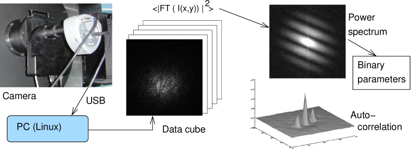
Figure 1: Schematic representation of data acquisition and processing.

2 Observations and data analysis

2.1 Speckle camera

The observations reported in this paper were obtained with the high-resolution camera (HRCam) – a fast imager designed to work at the SOAR telescope, either with the SOAR Adaptive Module or as a stand-alone instrument. The HRCam is described by Tokovinin & Cantarutti (2008); here we recall its main features.

HRCam uses a CCD detector with internal electron multiplication – an EMCCD. The Luca camera from Andor was chosen for its low cost, fast frame rate, and simple signal interface via a USB port. The CCD has 658x496 10-micron pixels. It is cooled thermoelectrically to $-20^{\circ}$C, resulting in a very low dark current for the short exposure time used here (except in a small number of hot pixels). We used an EM gain of 44, so the readout noise of 14 electrons is effectively reduced to 0.3 el. The quantum efficiency of this detector is around 0.5.

HRCam consists of the detector, mechanical structure, filter wheel, and optics. The $f/16$ beam coming from SOAR is collimated by a 50-mm negative achromat (Barlow lens) and refocused by a 100-mm positive lens, doubling the effective telescope focal length and providing a pixel scale of 15 mas. At the Blanco $f/8$ telescope, we replaced the negative lens by a positive achromat with 25-mm focal length to get adequate sampling.

HRCam has no corrector for atmospheric dispersion. Most observations were obtained through a Strömgren $y$ filter, while brighter stars were also observed through an H$\alpha$ interference filter, especially at large zenith distances. A few observations were taken through standard wide-band $V$, $R$ or $I$ filters. Table 1 lists the central wavelength and bandpass of each filter as measured (except for the $I$-filter where the bandpass is determined by the detector cutoff in the red).

Table 1: Filter information

Filter	Central Wavelength	FWHM,
	(nm)	(nm)
$V$	517.2	084.20
$y$	550.7	021.60
$R$	596.1	121.20
H$\alpha$	657.3	05.04 0
$I$	774.4	—

The camera software developed by R. Cantarutti works on a PC computer under the Linux operating system. All basic functionality is provided, including the filter wheel and detector control and connection to the telescope control system. We used the detector in free-run continuous mode. The central region of 200$\times$200 pixels may be read out with exposure time of 20 ms at a rate of 31.8 ms per frame, or a larger 400$\times$400 region may be read at a 43.1 ms frame rate. The required number (typically 400) of frames is grabbed during $13-17$ seconds and written to the disk. Immediately after the acquisition, a quick-look power spectrum is calculated and displayed, showing the quality of the data and the fringes for resolved binaries.

2.2 Observing procedure

Observing runs are listed in Table 2. As noted above, the use of HRCam at the Blanco telescope was not foreseen. The software was not interfaced to the telescope, so information missing in the FITS headers (acquisition time, object coordinates, zenith distance) was retrieved later using our logbook. A few object identification errors were corrected post factum, but some may still remain undetected. We planned to use the ADC of the Blanco telescope, but found it to be nonoperational, so the dispersion remained uncorrected and the program was restricted to smaller zenith distances. All 5 nights of the Blanco run were clear, with variable seeing.

Table 2: Observing runs

Run	Dates	Pixel Scale	$N_{dat}$
		(mas)
Blanco08	14-18 Jul 2008	16.35	2131
SOAR08a	8 Aug 2008	15.23	328
SOAR08b	6-8 Oct 2008	15.23	985
SOAR09	4-6 Apr 2009	15.23	1416

The SOAR telescope is located at the Cerro Pachón mountain. The shape of its thin 4.1-m mirror is controlled actively using a bright star at the beginning of the night and using look-up tables for the rest of the night. HRCam was installed at the Nasmyth focus and received the light after 3 reflections. SOAR has an alt-azimuth mount; field rotation at the Nasmyth focus is compensated by counter-rotating the instrument. The position angle of the rotator is recorded in the headers for subsequent calculation of angles on the sky.

In preparation for the SOAR runs, we tested the system during a technical night on August 8, 2008. Some useful data were collected during this night, mostly on binaries with known orbits. During the two scheduled 3-night runs in October 2008 and April 2009, the sky was clear, the wind speed was low, and the seeing was generally good, with the width of the best long-exposure images as small as 0^′′.70.

Efficient use of the allocated telescope time required good preparation of the observing program and a substantial effort on the part of the telescope operators. For example, during the April run, we observed 551 objects on 3 nights, spending less than 3.5 minutes per star on the average. Each observation included telescope slew, object acquisition, data recording, and quick-look analysis. We recorded at least two data cubes of each object and analyzed each cube independently. This strategy helped to verify new companion detections and to estimate observational errors. The last column of Table 2 lists the total number $N_{dat}$ of data cubes taken during each run.

The faintest stars observed were around $V=10^{m}$, with a few exceptions. For example, the components of DON 93 BC, $V=12^{m}$ and $13.1^{m}$ at 0^′′.76 separation, were measured reliably with an accuracy of 1 mas under good seeing. Companions of $V\sim 13^{m}$ were measured routinely if the primary star was brighter than $9^{m}$. Paradoxically, the presence of a bright primary increases the sensitivity for the secondary because the speckle signal is proportional to the product of photon fluxes from both companions. For faint stars, sensitivity could be gained at the expense of resolution by increasing the exposure time (up to 100 ms) and by observing in wide-band filters. This last resource was, unfortunately, not available to us because it requires a working compensator for atmospheric dispersion.

2.3 Calculation and modeling of the power spectra

Each data cube typically contains $K=400$ images of 200$\times$200 or 400$\times$400 format, with 14 bits per pixel. The average dark frame (with the same exposure time), called bias, is subtracted from each image to remove the fixed offset of $\sim$505 analog-to-digital units (ADU) and the dark current. The average bias is stable to within 1 ADU. Pixels in the bias frame which are more than 10 ADU above the average level are identified as “hot”; these pixels in the images are replaced by the average of neighboring pixels. Finally, all pixels below 17 ADU (twice the readout noise) are set to zero in order to reduce the influence of remaining pattern and readout noise. The optimum threshold value was selected after some trials and then applied to all data. Single photons produce signals well above this threshold. Despite the thresholding and the very low dark current, each 200$\times$200 frame contains some 40 photon events at random locations, apparently created in the electron-multiplication process. This additional background is the main factor which prevents observing very faint stars with long accumulation times. For a subset of bright stars observed without EM gain, only a fixed bias of 505 ADU was subtracted, without any thresholding.

Figure 2: Example of a power spectrum. Azimuthally averaged $P(f)$ is plotted in dashed line (raw) and in full line after division by $\overline{T}_{AD}(f)$. The model (2) is plotted in dotted line. Observations at SOAR in the $y$ filter, zenith distance $z=50^{\circ}$.7.

The power spectrum (PS) of an image cube is calculated by summing the square modulus of the Fourier Transform of each image,

$$P(f_{x},f_{y})=\frac{C}{K}\;\sum_{i=1}^{K}|\tilde{I}_{i}(f_{x},f_{y})|^{2}~{}.$$ (1)

The spatial frequencies $f_{x},f_{y}$ correspond to the elements of square discrete arrays. The normalization constant, $C$, is determined from the condition $P(0,0)=1$. In the following, it is convenient to use normalized frequencies $\kappa=f/f_{c}$, where $f_{c}=D/\lambda$ is the cutoff frequency, $D$ is the telescope diameter and $\lambda$ is the central wavelength of the filter passband.

It is well known that the PS of a single bright star $P_{0}(f_{x},f_{y})$ contains two components: a strong signal at low spatial frequencies $f<r_{0}/\lambda$ which corresponds to the seeing-limited image ($r_{0}$ is the Fried parameter) and a high-frequency component extending up to $f_{c}$ and produced by the speckle structure. An additive component $P_{noise}$ is produced by the photon noise. It is easily estimated by averaging the PS values at $f>f_{c}$. This additive term is then subtracted from the PS.

Knowledge of the speckle transfer function (STF) $P_{0}$ is needed for fitting a binary-star model to the data (see below). Single reference stars are sometimes observed for this purpose. However, the STF is not stable in time and depends on such factors as seeing conditions, atmospheric dispersion (AD), telescope aberrations, vibrations, etc. For each PS, we describe the STF in the high-frequency zone by an empirical model, obviating the need for a reference star and accounting for the changing conditions automatically. The bias term $P_{noise}$ is subtracted from $P(f_{x},f_{y})$, then the PS is averaged azimuthally, leading to the one-dimensional function $\overline{P}(\kappa)$. A very simple 2-parameter model

$$\log_{10}P_{r}(\kappa)\approx\log_{10}[\overline{T}_{AD}(\kappa)T_{0}(\kappa)]+p_{0}+p_{1}\kappa$$ (2)

is fitted in the range $\kappa_{\rm min}<\kappa<\kappa_{\rm max}$. Typically, we select $\kappa_{\rm min}=0.2$ and $\kappa_{\rm max}=0.8$, but for the noisy data the upper limit is reduced. Here $T_{0}(\kappa)=2/\pi[\arccos\kappa-\kappa\sqrt{1-\kappa^{2}}]$ is the diffraction-limited transfer function of an ideal telescope (the central obstruction is ignored), and $\overline{T}_{AD}(\kappa)$ is the azimuthally-averaged deterministic blur $T_{AD}(f_{x},f_{y})$ caused by the atmospheric dispersion (AD),

$$T_{AD}({\bf f})\approx\exp[-2\pi^{2}({\bf f}{\bf x}/2.506)^{2}].$$ (3)

The AD blur is represented by a Gaussian function. The length of the blur vector $|{\bf x}|=[n(\lambda_{1})-n(\lambda_{2})]/p\;\tan z$ (in pixels) is known for the zenith distance $z$, refractive index of air $n(\lambda)$, filter bandwidth limits $\lambda_{1}$ and $\lambda_{2}$, and the pixel size $p$. The direction of the vector ${\bf x}$ is known from the calculated parallactic angle and the detector orientation. Figure 2 illustrates power-spectrum modeling.

The parameter $p_{0}$ shows the level of the high-frequency component of the PS extrapolated to zero frequency. The theoretical PS model predicts that $(D/r_{0})^{-2}=0.435\,10^{p_{0}}$, leading to an estimate of the seeing conditions relevant to each data cube from the $p_{0}$ values. These seeing estimates match quite well the half-width of the re-centered long-exposure images calculated from the data cubes. The second parameter, $p_{1}$, shows how fast the high-frequency component of the PS is decreasing. For an ideal speckle pattern $p_{1}=0$, but in reality finite exposure time, finite bandwidth and other factors lead to $p_{1}<0$.

The synthetic STF is thus calculated as

$$P_{0,syn}({\bf f})=T_{AD}({\bf f})T_{0}(f)10^{p_{0}+p_{1}(f/f_{c})}$$ (4)

for the selected frequency range and $f=|{\bf f}|$. Alternatively, we use the azimuthally-averaged observed PS $\overline{P}(f)$ as a reference, with an additional multiplier $T_{AD}({\bf f})/\overline{T}_{AD}(f)$ to account for the AD. For binaries with separations above 0$\farcs$1 the radially-averaged reference is normally chosen, while synthetic reference is used for closer binaries.

2.4 Fitting parameters of binary and triple stars

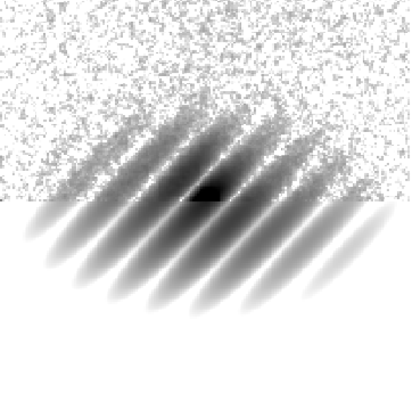
Figure 3: The PS of binary star FOX 102AB ($\rho$ = 0^′′.17, $\Delta m=0.45$) is displayed, replaced by the fitted model (5) with synthetic STF in the lower half. The intensity scaling is inverse logarithmic from $10^{-6}$ to $10^{-3}$. The AD blur in the $y$-filter was 3.4 pixels ($z=38^{\circ}$) in approximately vertical direction, causing elongation of the PS.

The PS of a binary star shows characteristic fringes. It is more practical, nevertheless, to detect companions in the auto-correlation functions (ACFs) calculated from the PS by Fourier transform. The two-component structure of the PS is carried to the ACF which consists of a wide seeing pedestal and three narrow peaks (in the case of binary star). The pedestal can be removed by setting to zero the PS at low spatial frequencies, e.g. at $f<0.2f_{c}$. Such crude filtering leads to “ringing” in the ACF. To avoid it, we divide the PS by its azimuthal average $\overline{P}(f)$ at low frequencies where it exceeds the extrapolated level of the speckle signal, $10^{p_{0}}$, and apply additional Gaussian damping to further reduce the low frequencies. The filtered ACFs are then computed from the filtered PS and are used together with the PSs for binary-star analysis.

The parameters of a binary star are the time of observation, $T$, separation, $\rho$, position angle, $\theta$, and magnitude difference, $\Delta m$. The first number is arbitrarily precise, the next two numbers are combined in a 2-dimensional vector ${\bf r}=(\rho\cos\theta,\rho\sin\theta)$. The observed power spectrum $P({\bf f})$ (after subtraction of $P_{noise}$) is fitted by a model

$$P_{mod}({\bf f})=P_{0}({\bf f})\;[A+B\cos(2\pi{\bf f}{\bf r})]~{},$$ (5)

where $P_{0}({\bf f})$ is the STF and the coefficients $A$ and $B$ are related to the magnitude difference. The position angle is determined only modulo $180^{\circ}$, so a change of quadrant is always possible.

Fitting of the model (5) to the PS is done by the Levenberg-Marquardt method in the frequency range $\kappa_{min}<\kappa<\kappa_{max}$ over the upper half-plane $\kappa_{y}\geq 0$, due to the symmetry. The error of the measured PS at each point $j$, $\sigma^{2}_{j}=(P_{j}+P_{noise})/K$ is taken into account ($K$ – number of images in the data cube). The quality of the fit is evaluated by the normalized sum of residuals $\chi^{2}/N=(1/N)\;\sum_{j}(P_{j}-P_{mod,j})^{2}/\sigma_{j}^{2}$, $N$ being the total number of the fitted points in the frequency plane. For noisy data, we obtain $\chi^{2}/N\sim 1$, but for bright stars the un-modeled systematic features of the STF (e.g. details caused by telescope aberrations) dominate the residuals, leading to $\chi^{2}/N$ values up to 20. Figure 3 shows the example of a binary-star PS and its fitted model. The fact that AD is explicitly included in the model helps to distinguish true close companions from the elongation of speckles produced by the AD.

A model of a resolved triple star is fitted in a similar way, but the number of parameters is larger. Initial values of the fitted parameters are determined by clicking on the companion(s) on the displayed ACF. In the data table we list positions and magnitude differences of triple-star pairs relative to the brightest component, not the photo-centers of close sub-systems. For example, the measurements of J01198$-$0031 = STF 113 A,BC at 1$\farcs$67 in fact refer to the pairing (A,B), not to the center of the inner sub-system FIN 337 BC. Accordingly, in the data tables we designate the wide pair as STF 113 AB. The quadrants in a triple system can be changed jointly, but not individually. When the quadrant of the slowly moving outer pair is known from previous observations, the quadrant of the inner pair can be established without ambiguity.

The fitting program provides estimates of the parameter errors. Yet another estimate comes from the variance of $N$ measurements obtained on the same night in the same filter, $\sigma_{x}^{2}=(N-2)^{-1}\sum_{N}(x-\overline{x})^{2}$. Mostly, $N=2$ (two data cubes). We adopt the larger of these two errors and list them in the data table. For 1846 measurements with $N\geq 2$, the median errors of companion positions are 0.3 mas in both radial and tangential directions, while 75% of the errors are smaller than 0.8 mas. For a subset of 49 measurements with $N\geq 4$ where the estimates of the variance are more reliable, the median errors in tangential and radial directions are 0.5 mas and 0.6 mas, respectively. The error in separation exceeds 7.5 mas (half-pixel) in only 16 cases where the companions are either close or very faint. The listed errors are internal, they do not take into account calibration uncertainties or other systematic effects. During the Blanco run, some bright pairs were observed repeatedly, and the argeement between these measurements is quite good. For example, A 417 (WDS 23052$-$0742) shows the scatter $\sigma_{\rho}=0.30$ mas and $\rho\sigma_{\theta}=0.23$ mas from 6 measurements over 4 nights in two filters.

2.5 Calibration

Figure 4: Inter-comparison of separations measured in the Blanco08 and SOAR08b runs on 107 common pairs. The dotted lines show $\pm 1$% deviations in the pixel scale. The estimated measurement errors are shown by the vertical lines.

Accurate knowledge of the detector pixel scale and orientation is needed to convert binary-star parameters from fitted values in pixels to absolute positions on the sky. Speckle measurements at the Mayall 4-m telescope at Kitt Peak National Observatory were calibrated by means of a double-slit mask (Hartkopf et al., 2000), while speckle data at the Blanco telescope were traditionally tied to this calibration by observing common pairs. Originally, we intended to observe many binaries with known orbits to calibrate our runs. However, it turned out that the quality of the available binary star orbits is not adequate. By calibrating against orbits, we relate modern precise measurements to the historical data of much lower accuracy which may also contain systematic errors.

A comparison between the Blanco08 and SOAR08b runs has revealed a disagreement of the pixel scale at the 3.5% level, despite independent calibration of each run with $\sim 100$ orbits. In the face of this discrepancy, we calibrated the SOAR09 run by projecting into the telescope a fringe pattern formed by two coherent point sources attached to the telescope spider. The baseline of this interferometer $b=0.4999\,$m was accurately measured, the wavelength of the green laser $\lambda=532.2$ nm is known, so the fringe period $\lambda/b=$0$\farcs$2196 is known as well. About 30 fringes fit into the 400$\times$400 pixel field. The position of the fringe peak in the PS of these data cubes is found by a simple centroid, leading to the determination of the pixel scale and detector orientation.

The results for each of the 8 series of fringe measurements are very consistent internally, but do show a spread between the series amounting to 0.5% in scale and $0\fdg 2$ in angle. We attribute these differences to small imperfections in the fringe pattern caused by optical defects and aberrations in the beam path. The pixel scale of 15.23 mas is finally adopted for all SOAR runs. We measured also the effective pixel size of the HRCam detector (through its optics) by illuminating the device with a laser and determining the angle between the beams diffracted back by the pixel grid. The nominal projected pixel size of $5.00\pm 0.025$ $\mu$m was confirmed. Using the effective focal length of the SOAR known from its optical prescription, $F=67.834$ m, we obtain the pixel scale of 15.20 mas in agreement with the laser calibration.

The detector orientation in the SOAR09 run was independently checked by observing stars at large zenith distances with wide filters. The resulting PS is elongated perpendicularly to the AD direction which itself is known. The elongation angle is determined by correlating the observed and modeled PSs in a certain range of spatial frequencies and finding the angle where the correlation reaches maximum. It turned out that most consistent results are obtained by considering the mid-range spatial frequencies between 0.1 and 0.3$f_{c}$, while at higher frequencies the direction of the elongation is possibly affected by telescope vibrations (see below). The resulting detector angle determined from AD is $1\fdg 32\pm 0\fdg 1$, to be compared to $1\fdg 37\pm 0\fdg 1$ measured from fringes and $1\fdg 52\pm 0\fdg 2$ from orbits. In this case, all three methods agree very well.

The pixel scale of the Blanco run was adjusted using 107 binaries measured also in October 2008 (Fig. 4). The unweighted rms difference $\rho_{Blanco}-\rho_{SOAR}$ after adjustment is only 3.5 mas. A similar level of agreement is seen between other pairs of runs. This is the upper limit for the external measurement errors (part of the difference is caused by the motion of binaries between the runs). In contrast, the residuals in $\rho$ to the orbits (Fig. 5) show a large scatter for the whole data set and for the individual runs, precluding accurate scale calibration. Calibration only with the orbits of grade 1 does not help. The rms scatter of the O$-$C residuals in $\rho$ in Fig. 4b is still 8.3 mas for 32 points with $\rho<0\farcs 4$, much larger than the difference between the runs. The residuals to orbits in the tangential direction are around 5 mas.

Figure 5: Residuals (O$-$C) in separation with respect to orbits. In the upper panel, the whole data set (432 points) is plotted, with orbits of grades 3 and higher as larger squares. The two dotted lines indicate $\pm 1$% range in the pixel scale. In the lower panel, only the 64 points with orbits of grade 1 are retained.

The detector orientation changes slightly at each installation of the camera, so it has to be calibrated for each run. Considering the comparisons with orbits, the difference in $\theta$ between wide binaries measured commonly in pairs of runs, and the secure angular offset determined for the SOAR09 run, we adjusted the offsets in $\theta$ iteratively to reach mutual consistency between all runs. The remaining average differences in $\theta$ between any pair of runs are less than $0\fdg 2$, while the pixel scales are consistent to within 0.2% or better. We believe that the absolute calibration errors do not exceed 1% in scale and $0\fdg 5$ in angle, and that they are likely smaller. The data presented in this paper are possibly the most accurate measurements of southern binaries done so far.

2.6 Relative photometry of binary components

The contrast of fringes in the PS $\beta=B/A$ (or the ratio of peaks in the ACF $\beta/2$) is related to the magnitude difference between binary components $\Delta m$,

$$\Delta m=-2.5\log_{10}[(1-\sqrt{1-\beta^{2}})/\beta]~{}.$$ (6)

For small $\Delta m$, the slope of this relation is shallow, leading to a larger error of relative photometry. Moreover, as the fringe contrast is often under-estimated, the $\Delta m$ is over-estimated. The positive bias on $\Delta m$ becomes significant for faint stars, where the PS models fail. It is likely that the background photons cause this effect, given that PS is related to the intensity in a non-linear way (Eq. 1). For faint stars, the slope of the PS models $|p_{1}|$ is systematically less than normal, indicating that something is wrong.

We compared our speckle photometry with that of Hipparcos (ESA, 1997), using only the Strömgren $y$ data as that filter most closely matched the Hipparcos $Hp$ filter. We found that the positive bias on $\Delta y$ is strongly correlated with the signal-to-noise ratio $\delta$, which we define here as the ratio of the speckle signal to the photon-noise bias at 1/2 of the cutoff frequency,

$$\delta=T_{0}(0.5)\;10^{p_{0}+0.5p_{1}}/P_{noise}~{}.$$ (7)

Figure 6 shows such correlation for the Blanco run. Observations with $\delta<0.25$ are marked by colons in the data table. These biased estimates are still useful as upper limits, especially for close pairs where no other photometry is available.

Figure 6: Comparison of the magnitude difference $\Delta y$ measured by speckle at Blanco with magnitude difference $\Delta Hp$ measured by Hipparcos for common pairs with $\rho<0\farcs 8$, as a function of the signal-to-noise ratio $\delta$.

Another reason for $\Delta m$ over-estimation is the loss of correlation between speckle patterns of wide binary components (anisoplanatism). We implemented an alternative scheme for estimating $\Delta m$ directly from average re-centered images, provided that the binary is resolved ($\rho$ larger than the half-width of long-exposure image). The relative position of the components is already known from the PS fitting, so we have to determine only the true quadrant and $\Delta m$. The quadrant is selected by comparing two point-spread functions (PSFs) obtained by de-convolving the average image from the binary. For the wrongly selected quadrant, the PSF has a negative lobe opposite to the companion, so we select the quadrant with the least negative PSF. The de-convolved PSFs are then computed for a grid of $\Delta m$ values from 0 to the $\Delta m$ estimated from speckle. The final $\Delta m$ value is the one which gives the most symmetrical PSF, when the secondary component disappears. This procedure is applied automatically to all data, but in some cases (wrong quadrant choice for $\Delta m\sim 0$ or large $\Delta m$) it fails. In the following, we call this method resolved photometry and mark such $\Delta m$ estimates to distinguish them from the standard speckle photometry of closer pairs.

Figure 7 compares $\Delta y$ measured by speckle (only data with $\delta>0.25$) and by resolved photometry with the Hipparcos photometry, for the whole data set. These plots help to evaluate the accuracy of our photometry. Despite some remaining deviant points, the overall agreement is evident. Wide pairs without resolved photometry suffer from the positive $\Delta y$ bias caused by anisoplanatism. As this bias is variable, depending on high-altitude turbulence, we do not attempt to quantify it.

Quantitative evaluation of the bias and precision of our photometry is given in Table 3. We compare speckle photometry of close ($\rho<1^{\prime\prime}$) pairs with good S/N ($\delta>0.25$) and resolved photometry of wide pairs with magnitude differences $\Delta Hp$ measured by Hipparcos (first two lines) and with magnitude differences $\Delta V$ derived from the Tycho data by Fabricius & Makarov (2000) (last two lines). Each line lists the number $N$ of pairs in common, median and average difference between $\Delta m$’s, and the rms dispersion of the difference. The speckle photometry has a small positive bias, while the resolved photometry is essentially unbiased. The speckle photometry bias is larger in comparison with the Tycho $\Delta V$ than with $\Delta Hp$ because only pairs wider than 0$\farcs$3 are considered by Fabricius & Makarov (2000), hence larger contribution of anisoplanatism. When we compare our $\Delta y$ with $\Delta Hp$ only for pairs with $0\farcs 3<\rho<1^{\prime\prime}$, a similar positive bias of $0.2^{m}$ appears, but the rms scatter becomes smaller, around $0.20^{m}$. The Hipparcos photometry of close pairs with $\rho<0\farcs 2$ (below the resolution limit of the Hipparcos telescope) is suspect, as can be seen in the lower plot of Fig. 7. We estimate that intrinsic random errors of our photometry (both speckle and resolved) are around $0.2^{m}$ r.m.s., but in a few cases the disagreement between our and published photometry is much larger.

Table 3: Comparisons of relative photometry

Data	$N$	Med.	Aver.	r.m.s.
		(mag)	(mag)	(mag)
Sp. $\Delta y-\Delta Hp$	303	0.13	0.11	0.34
Res. $\Delta y-\Delta Hp$	162	0.04	0.08	0.42
Sp. $\Delta y-\Delta V_{\rm Tyc}$	206	0.23	0.28	0.30
Res. $\Delta y-\Delta V_{\rm Tyc}$	132	0.02	0.05	0.19

Figure 7: Comparison of the magnitude difference $\Delta y$ measured by speckle (crosses, $\delta>0.25$) and by resolved photometry (squares) with magnitude difference $\Delta Hp$ measured by Hipparcos for the whole data set. Top: common pairs with $\rho<1^{\prime\prime}$, bottom: $\Delta y-\Delta Hp$ as a function of separation $\rho$.

2.7 Detection limits

Binary companions are detected as symmetric spikes in the filtered ACF. Fluctuations in the ACF caused by photon noise, residual speckle statistics, etc. prevent detection of faint companions. The rms fluctuations in the annuli of 2-pixel width around the central peak are calculated for each ACF; this $\sigma(\rho)$ curve is translated to the detection limit $\Delta m_{3}(\rho)$ by assuming that all companions above $3\sigma$ are detectable. Of course, the annulus containing the actual companion will have enhanced fluctuations and lower $\Delta m_{3}$. However, as shown in Fig. 8, a simple linear model can be fitted to the $\Delta m_{3}(\rho)$ curve by excluding the companion zone. Typically, the slope of the curve changes abruptly at some distance $\rho^{*}\sim 0.15^{\prime\prime}$, so we approximate it by two linear segments intersecting at $\rho^{*}$. Such 2-segment linear models are fitted to all data.

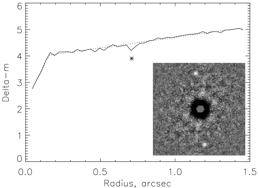
Figure 8: Fluctuations in the filtered ACF of a faint binary star are calculated, translated to the $3\sigma$ detection limit $\Delta m_{3}$ and plotted as a function of radius. The asterisk marks $(\rho,\Delta m)$ of the actual binary companion. Approximation of the curve by two linear segments is plotted as a dotted line. The insert shows a fragment of the ACF, with the central peak masked.

The detection threshold was checked by simulating fake companions. A real ACF of a single star (or a binary de-convolved from a faint companion) was used as a model of the speckle PSF, then companions were generated with separations from 0$\farcs$1 to $1^{\prime\prime}$ and $\Delta m$ in the $(-1.0,+0.5)$ interval around $\Delta m_{3}$. About 10 representative cases were tested in this way, with 100 trial companions each (Fig. 9). Our general conclusion is that the $5\sigma$ line $\Delta m_{5}=\Delta m_{3}-0.55$ corresponds to certain detection, companions in the region between $\Delta m_{5}$ and $\Delta m_{3}$ are detected fairly frequently, and companions with $\Delta m>\Delta m_{3}$ remain undetected, with few exceptions.

Figure 9: Verification of the companion detection limit (example). Solid and dashed lines indicate the $\Delta m_{3}$ and $\Delta m_{5}$ curves, respectively. Positive detections are plotted as asterisks, failed detections as squares.

Figure 10 compares the detection limits estimated by the above procedure with the actually measured $\Delta m$. Only data with good signal-to-noise $\delta>0.25$ and $\rho>0\farcs 15$ are selected. Positive bias in $\Delta m$ inherent to speckle photometry is also relevant to the detection limits which are over-estimated by the same amount. For wide companions with $\rho>1^{\prime\prime}$ anisoplanatism becomes important, making our formal detection limits optimistic. The same is true for the noisy data with $\delta<0.25$. We list the $\Delta m_{5}$ detection limits for unresolved targets at separations of 0$\farcs$15 and $1^{\prime\prime}$ and mark cases with $\delta<0.25$ by colons. The actual detection limits for companions closer than $0.1^{\prime\prime}$ cannot be established by the above simple analysis, as they depend on a number of artifacts discussed in the next sub-section. Median detection limits $\Delta m_{5}$ for the whole data set are $4.22^{m}$ and $5.33^{m}$ at 0$\farcs$15 and $1^{\prime\prime}$, respectively. For the best 25% of data, these limits exceed $4.67^{m}$ and $6.08^{m}$.

Figure 10: Comparison of the measured $\Delta m$ (horizontal axis) with the detection limits (vertical axis). Only those 777 pairs with $\rho>0\farcs 15$ and valid speckle photometry are plotted.

2.8 Artifacts and false companions

In all data sets, most ACFs are round, but some ACFs show symmetric enhancements near the first diffraction ring which can be mistaken for a binary companion with $\Delta m\sim 3$. In the case of binary stars, these false details appear around the secondary peaks as well, distinguishing them from true triple systems where the secondary peaks are doubled, not tripled.

These false peaks have some common features. First, their separation from the center, typically from 45 mas to 75 mas, is larger in the H$\alpha$ filter than in the y filter, while the intensity of the peaks is also larger in H$\alpha$. Secondly, the peaks are almost always oriented vertically, along the AD direction. Yet, they are not caused by the AD because the separation does not depend on the spectral bandwidth and the zenith distance (the peaks are seen even near the zenith). Third, the separation, orientation, and intensity of the peaks is variable. In two data cubes of the same star, one may have the false peaks while the other does not. When we split the data cube into 10 segments and calculate the PS for each segment, the variability of the peaks on a time scale of seconds becomes even more apparent. However, the peaks often appear persistently in the ACFs of different objects observed one after another in the same part of the sky.

The persistent nature of these peaks means that they are not caused by random fluctuations of speckles and do not disappear when more data are averaged. Having at least two data cubes for each object and examining data on other objects observed before and after the star usually helps to identify and reject false companions, despite their striking resemblance to real binaries in some cases.

The properties of the false peaks indicate that they are likely caused by variable optical aberrations with characteristic size of 2 m, or ½ of the telescope diameter. We simulated speckle data by adding a sinusoidal wave-front aberration with $\frac{D}{2}$ period to the atmospheric distortions. Some characteristics of the false peaks (Fig. 11, right) could be reproduced. The intensity of the false peaks is larger in H$\alpha$ than in y, and it decreases with degrading seeing. Orientation of the peaks in the vertical direction suggests that optical aberrations such as astigmatism could play some role, but our simulations show that the STF can be affected only by a fairly large amount of defocus and astigmatism causing visible elongation of the seeing-limited PSF. Even then the astigmatism produces an elongation of speckles, rather than their tripling. Air stratification in the dome can possibly cause this optical effect, but its exact nature remains mysterious. Such false peaks could explain previous detections of speckle companions which turned out to be bogus. See the discussion of false speckle companions by McAlister et al. (1993).

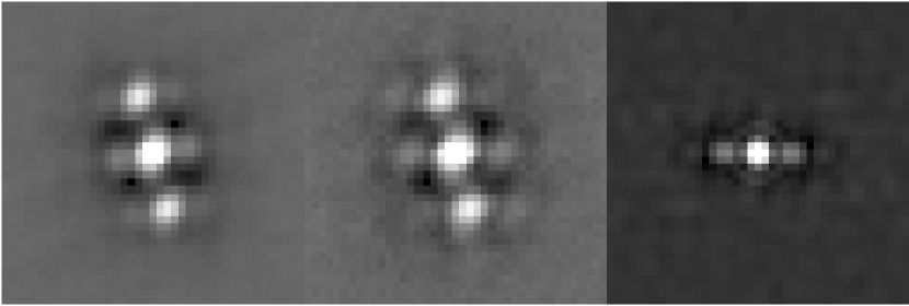
Figure 11: Illustration of false peaks in the ACFs. Central $0\farcs 6\times 0\farcs 6$ portions of the filtered ACFs of the binary star BU 368AB ($\rho=0\farcs 12$) observed in August 2008 in the filters $y$ (left) and H$\alpha$ (center) are shown. The right panel shows the simulated ACF of a single star in H$\alpha$ with optical aberrations of $\frac{D}{2}$ period and amplitude 0.8 $\mu$m, under $0\farcs 8$ seeing, and on the same scale. All images have the same square-root intensity stretch from minimum (black) to 0.5 of the ACF maximum (white).

Sometimes speckle peaks in the ACF are also elongated at a large angle with respect to the AD. This blur could be caused by telescope aberrations or tracking errors. Although tracking errors are usually slow (typical frequency 1 Hz), their amplitude can be large enough to degrade the resolution in a 20-ms exposure. Alternatively, speckles can be elongated by fast turbulence. Instrumental elongation of speckles is indistinguishable from the effect of a close binary companion at the limit of resolution ($\sim 30$ mas), so only the examination of data on stars observed before or after can help to distinguish an authentic close binary from an artifact.

Clearly, detection and measurement of close binary companions are complicated by the artifacts and involve an element of human judgment and error. The detection limits cannot be formalized, as was done for wider companions. We cannot exclude the possibility that some of the measurements presented below are affected by the artifacts, despite all efforts to understand and eliminate them.

3 Results

3.1 Data tables

Table 4 lists 1898 measurements of 1189 resolved known and new binary stars and sub-systems. Its columns contain (1) the WDS (Mason et al., 2001a) designation, (2) the “discoverer designation” as adopted in the WDS, (3) an alternative name, mostly from the Hipparcos catalog, (4) Besselian epoch of observation, (5) filter, (6) number of individual data cubes, (7,8) position angle $\theta$ in degrees and internal measurement error in tangential direction $\rho\sigma_{\theta}$ in mas, (9,10) separation $\rho$ and its internal error $\sigma_{\rho}$ in mas, and (11) magnitude difference $\Delta m$. An asterisk follows the value if $\Delta m$ and the true quadrant are determined from the resolved photometry; a colon indicates that the data are noisy and $\Delta m$ is likely over-estimated. We decided not to mark with colons the $\Delta m$ values of wide pairs over-estimated only due to anisoplanatism (when no resolved photometry is available), to avoid confusion with the low S/N cases. Note that in the cases of multiple stars, the positions and photometry refer to the pairings between individual stars, not with photo-centers of sub-systems.

For stars with known orbital elements, columns (12–14) of Table 4 list the residuals to the ephemeris position and the reference to the orbit from the 6^th Orbit Catalog (Hartkopf, Mason, & Worley, 2001). In those cases where multiple orbits for the same system are present in the catalog, the orbit with the smallest residuals is selected. An asterisk in the final column indicates that a note concerning this system may be found in Table 7.

Table 5 contains the data on 285 unresolved stars, some of which are listed as binaries in the WDS or resolved here in other runs. Columns (1) through (6) are the same as in Table 4 (although Column (2) also includes Bayer designations, HD numbers, or other names for objects without discoverer designations). Columns (7,8) give the $5\sigma$ detection limits $\Delta m_{5}$ at $0\farcs 15$ and $1^{\prime\prime}$ separations determined by the procedure described above. When two or more data cubes are processed, the best detection limits are listed. Noisy data with $\delta<0.25$ are marked by colons to indicates that the actual detection limits are smaller. As in Table 4, the final column indicates a note to the system.

New discoveries are repeated in Table 6 in the same format as measurements in Table 4 – a total of 48 pairs. Figure 13 shows ACFs of 20 newly resolved triple systems.

3.2 Comments on individual objects

Notes to some objects in Tables 4, 5, and 6 are given in Table 7. These notes include miscellaneous information such as additional components, discovery history, etc. The WDS (Mason et al., 2001a) and the Multiple-Star Catalog (Tokovinin, 1997) were extensively consulted, among other sources. Each system is identified by its WDS designation and an alternate name. Cases where deviations from the orbits are quite large are also indicated. The definition of unacceptably large residuals is subjective; we consider as such orbits which deviate from our measurements by more that $20^{\circ}$ in $\theta$ or by more than 50% in $\rho$. There are 131 such cases out of 544 systems with orbits. The 24% fraction of bad orbits demonstrates that more measurements of southern binaries are needed.

In this sub-section we give more lengthy comments on a few selected cases.

02053-2425 = HIP 9774 = I 454: The brightest companion of I 454 (also known as ADS 1652) is a double-lined spectroscopic binary with period 2.6 yr and eccentric orbit, $e=0.78$ (Tokovinin, unpublished). The estimated semi-major axis of this pair is 47 mas. The system passed through periastron in May-June 2008 and was marginally resolved in July 2008 at Blanco. In October 2008 the separation was closer, below the diffraction limit of the 4-m telescope. Nevetheless, we were able to fit consistently a triple-star model to 7 power spectra recorded in October. As our estimated $\Delta m\sim 1^{m}$ is larger than the spectroscopically estimated $\Delta m\sim 0.3^{m}$, it is possible that the actual separations were even smaller than those listed in Table 6. Component C = HIP 9769 of this multiple system was also observed here and found to be single.

02225-2349 = HIP 11072 = $\kappa$ For = TOK 40: The companion was first resolved in 2007 (Tokovinin & Cantarutti, 2008). New measurements are roughly compatible with the 26.5-yr astrometric orbit of Gontcharov & Kiyaeva (2002) if we adjust the semi-major axis to $0\farcs 65$ and the node position angle to $120^{\circ}$. New photometry ($\Delta y=5.0$, $\Delta{\rm H}\alpha=4.3$) shows that the companion is not as faint as measured initially, and that it is redder than the primary star. It will be very useful to measure the relative brightness of the companions in the near-IR with adaptive optics.

05086-1810 = HIP 23932 = WSI 72: Speculated to be a close binary by Henry et al. (2002), it was first resolved in 2006 with the USNO speckle camera on the Blanco 4m by Mason et al. (2010b) at about the same position angle and twice the separation measured here.

05354-0555 = HIP 26241 = CHR 250Aa,Ab: New measurements confirm slow rectilinear motion of this pair due either to a long-period orbit or to Ab being an unrelated background star, in agreement with the conclusions of Mason et al. (2009). Our photometry indicates that CHR 250Ab is bright, V$\sim 6^{m}$.

Figure 12: Observed motion of the E component (squares) relative to the C component (big star) in the CE sub-system of the visual quadruple star GJ 225.2 The separation decreases from 0$\farcs$514 in 2004.86 to 0$\farcs$239 in 2009.26. The line shows a possible orbit with 23.7-year period.

06003-3102 = HIP 28442C = GJ 225.2C = TOK 9CE: The E companion in this nearby quadruple system was discovered with adaptive optics in 2004 (Tokovinin et al., 2005). In that paper, a tentative astrometric orbit with 23.7-yr period was proposed, and an unusually “blue” $J-K$ color of E was noted. The component E was marginally resolved in the visible during the first speckle run at SOAR (Tokovinin & Cantarutti, 2008). In the present data, the companion is seen reliably above the detection limit, and its magnitude difference is measured consistently as $\Delta y=4.5^{m}$. All 4 position measurements available to date show retrograde orbital motion (Fig. 12) which does not follow the preliminary astrometric orbit suggested by Tokovinin et al. (2005), but is still compatible with a 24-year orbital period. Within a few years, the orbit can be established more firmly and we will be able to address the properties of this apparently peculiar companion. New observations of the other sub-system AB confirm its orbital elements.

06410+0954 = HIP 31978 = 15 Mon = CHR 168Aa,Ab: The most recent orbit of Gies et al. (1997) is clearly in error. This system has been the subject of regular observation by both speckle interferometry and HST-FGS. A new orbit is currently in preparation.

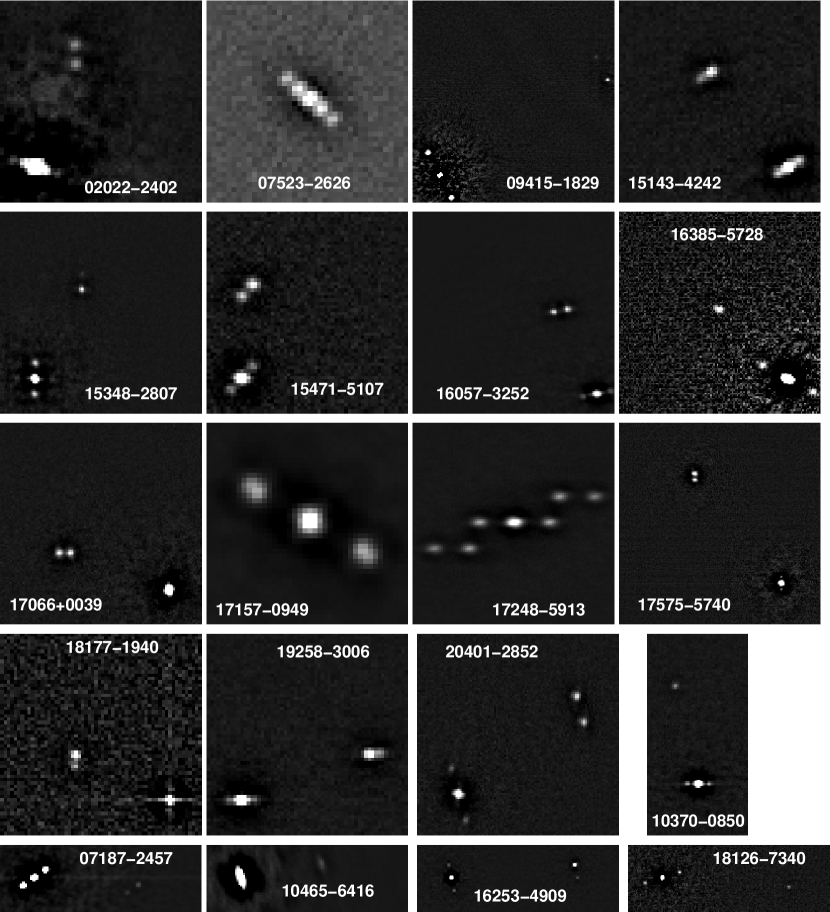
Figure 13: ACFs of 20 triple stars with newly resolved components. Each panel shows a fragment of the filtered ACF including the central peak and some or all companion peaks, in arbitrary intensity stretch and with detector lines horizontal (not necessarily North up).

07523-2626 = HIP 3840 = V402 Pup = WSI 54: This $9.23^{m}$ star of spectral type O6e belongs to the open cluster NGC 2467. Mason et al. (2009) have resolved it into a close pair WSI 54 and measured in 2006.194 the position angle $231.8^{\circ}$ and the separation $0\farcs 091$. Our observations clearly show three stars in a tight linear configuarion (Fig. 13). The outer companion matches the WSI 54 pair best, the inner companion has a separation 2 times smaller and a similar flux. This detection is based on 3 independent data cubes, the companions are not aligned with the AD, so we are confident that this is not an artifact. Further observations will reveal whether this is a dynamically unstable system (trapezium), an unsual multiple with orbits in resonance, or a chance projection of a binary and a single star, more probable in a cluster than in the field.

17248-5913 = HIP 85216 = I 385 + WSI 85: Quite unexpectedly this star, previously considered as a binary, turned out to be a spectacular triple with components of comparable magnitude and separation (trapezium-type); see Fig. 13. During the 0.72-yr time between the Blanco and SOAR09 runs, the relative position of both companions changed only slightly; the magnitude differences remained stable as well. Comparing our measurements with published data, we identify the wider companion at $122^{\circ}$, $0\farcs 39$ with the previously known component B and designate the new companion at $270^{\circ}$, $0\farcs 26$ as D. The distant companion C at $210^{\circ}$, $17^{\prime\prime}$ (also seen in the 2MASS images) is $5^{m}$ fainter than A and has moved only slightly since its discovery in 1901. Therefore, C likely belongs to this system.

The AB pair has revolved by $64^{\circ}$ over the 110 years since its discovery by Innes (1905), suggesting an orbital period of $\sim 600$ yr; this corresponds also to the dynamically estimated period at a distance of 211 pc measured by Hipparcos. The projected separation of AD (55 AU) means that its orbital period should be of the order of 300 yr.

The component D was noted in the only previous speckle observation by Hartkopf et al. (1993), but it was not accepted as real at that time. Re-measurement of the correlation peak corresponding to AD yields $0\farcs 199,\;270\fdg 18$ on 1990.3496. It seems that the pair AD is slowly opening up. The AD was not resolved visually at a 1-m telescope by Holden (1977a). The Hipparcos measured the relative position of AB at $118^{\circ}$, $0\farcs 452$ in disagreement with all other data, as though the light center of AD was measured instead of A. The mysterious new companion D deserves futher observations.

17535-0355 = HD 162905 = V2610 Oph = TOK 54: According to Pribulla et al. (2009), this is a close quadruple system composed of two double-lined binaries with periods 8.47 and 0.425 days (the latter is also eclipsing) orbiting each other. All components are dwarfs of spectral types F to G. The outer system is resolved here for the first time. The authors estimate $\Delta m=0.27^{m}$; our measurement $\Delta y=1^{m}$ is biased by the low S/N. Some other eclipsing binaries discovered to be spectroscopic multiples by the same team were also observed at SOAR in April 2009 and found unresolved. However, one of those, HDS 238, has a visual companion at 3$\farcs$2 listed in the WDS, too wide to be measured here.

18455+0530 = HIP 92027 = STF 2375AB, FIN 332Aa,Ab & FIN 332Ba,Bb: New orbits, based on new reductions of historical interferometric measures and new measures, are in process for this complex multiple system (Mason et al., 2010a).

20401-2852 = HD 196718 = SEE 423: This triple system ($V=8.70$, F5V) was first resolved in 1897 at $(0\farcs 92,20^{\circ}$). Three observations of this pair are listed in Aitken’s (1932) catalog under #14115, showing slow direct motion. Holden (1977b) measured in 1976.8 $(0\farcs 76,32^{\circ})$ and $\Delta m=0.5$. However, a larger separation of $(1\farcs 112,33^{\circ})$ was measured by the Tycho experiment on 1991.68 (ESA, 1997). One year later, in 1992.4552, Hartkopf et al. (1996) found the pair at a very different position, $(0\farcs 34,271^{\circ})$. We see now that this system is a visual triple (Fig. 13), with the wide pair AB at $(1\farcs 15,38^{\circ})$ matching the Tycho result and corresponding to SEE 423. The closer pair BC is fainter than A by $0.64^{m}$ (Tycho) and was apparently measured for the first time in 1992 by Hartkopf et al. (1996). The triple nature of SEE 423 clarifies some, but not all contradictions in the existing data. The wider (and the brightest) component was not seen by speckle in 1992 as it was outside the field-of-view. However, why did Holden and other visual observers not resolved the sub-system BC with nearly equal components? Also, why is the measured separation of the wide pair so discordant, ranging from 0$\farcs$76 (Holden) to 1$\farcs$15 (this work)?

Table 4: Measurements of known and new binary stars (fragment)

WDS	Discoverer	Other	Epoch	Filt	N	$\theta$	$\rho\sigma_{\theta}$	$\rho$	$\sigma\rho$	$\Delta m$	[O$-$C]θ	[O$-$C]ρ	Reference	Note
(2000)	Designation	name	+2000			(deg)	(mas)	(′′)	(mas)	(mag)	(deg)	(′′)	code∗
00006$-$5306	HJ 5437	HIP 50	8.7697	y	2	332.7	0.2	1.4904	0.7	string3.4  *
00008$+$1659	BAG 18	HIP 68	8.5378	y	1	6.8	6.0	0.6112	6.1	string4.6
00008$-$3244	I 1478	HD 224811	8.5459	y	2	328.6	0.3	0.3766	0.3	string1.1  :
00028$+$0208	BU 281 AB	HIP 223	8.5379	y	5	161.9	0.2	1.5689	1.0	string2.0  *				*
			8.7672	y	2	161.7	0.5	1.5709	0.2	string2.2  *
00039$-$5750	I 700	HIP 306	8.5459	y	2	144.1	0.2	0.2965	0.2	string0.8  :
00059$+$1805	STF 3060 AB	HIP 495	8.5377	y	2	133.6	1.5	3.4185	1.5	string0.3  *				*
00059$-$3020	RST 5180 AB	HD 117	8.5459	y	2	340.3	0.3	0.3274	0.3	string1.2  :				*
00090$-$5400	HDO 181	HIP 730	8.5379	y	2	35.4	0.3	0.3236	0.1	string1.8	$-$3.4string	$-$0.013string	Alz2000b
			8.5379	H$\alpha$	2	35.4	0.2	0.3228	0.2	string2.0	$-$3.4string	$-$0.013string	Alz2000b
			8.5431	y	2	35.5	0.4	0.3228	0.4	string1.7  :	$-$3.3string	$-$0.013string	Alz2000b
			8.5431	H$\alpha$	2	35.3	0.7	0.3223	0.8	string2.2  :	$-$3.5string	$-$0.014string	Alz2000b
			8.5486	y	3	35.3	0.1	0.3237	0.3	string1.6	$-$3.5string	$-$0.013string	Alz2000b
			8.6059	y	2	35.2	0.1	0.3241	0.2	string1.6	9.8string	$-$0.060string	Sey2001
00098$-$3347	SEE 3	HIP 794	8.5459	y	2	116.1	0.3	0.7827	0.3	string1.5  :	38.5string	0.100string	Csa1983a	*
			8.5459	H$\alpha$	2	116.1	0.7	0.7819	0.7	string1.5  :	38.5string	0.099string	Csa1983a
			8.5486	y	3	116.1	0.5	0.7830	0.7	string1.7  :	38.5string	0.100string	Csa1983a
00115$-$5545	HDS 25	HIP 927	8.5459	y	2	77.5	0.4	0.1775	0.2	string1.0
00121$-$5832	RST 4739	HIP 975	8.5431	y	2	134.8	0.6	0.3191	0.6	string1.4  :				*
			8.7697	y	2	133.9	0.1	0.3182	0.1	string0.4
00126$-$1142	RST 3343	HIP 1005	8.5432	y	2	253.0	0.4	0.2799	0.3	string1.0  :	$-$7.6string	$-$0.036string	Hei1998
			8.5487	y	3	253.1	0.2	0.2801	0.2	string0.7  :	$-$7.5string	$-$0.036string	Hei1998
			8.6059	y	2	253.1	0.1	0.2803	0.1	string0.4	$-$7.6string	$-$0.036string	Hei1998
00143$-$2732	HDS 33	HIP 1144	8.5432	y	4	116.2	0.4	0.1737	0.5	string1.4  :

* The complete list of references may be found at http://ad.usno.navy.mil/Webtextfiles/wdsnewref.txt .

Table 5: Unresolved stars (fragment)

WDS (2000)	Discoverer	Hipparcos	Epoch	Filter	N	5$\sigma$ Detection Limit		$\Delta m$	Note
	Designation	or other	+2000			$\Delta m(0\farcs 15)$	$\Delta m(1^{\prime\prime})$	flag
	or other name	name				(mag)	(mag)
00024$+$1100	HD 224983	HIP 184	8.5378	y	2	4.06	4.63
00059$+$1814	LTT 10019	HIP 493	8.5377	y	2	4.03	4.49
00063$-$4905	HDO 180	HIP 522	8.5379	y	2	4.60	6.19		*
00084$+$0637	HD 377	HIP 682	8.5378	y	2	4.60	5.46
00113$-$1528	6 Cet	HIP 910	8.5379	y	2	4.96	6.19
00116$+$1020	HD 727	HIP 943	8.5378	y	2	3.99	4.55
00117$-$3508	the Scl	HIP 950	8.5379	y	2	4.76	6.27
00125$+$1434	LN Peg	HIP 999	8.5378	y	2	3.66	4.19
00174$+$0853	STF 22 C	HIP 1392	8.7672	y	2	4.06	5.84		*
00201$-$6452	zet Tuc	HIP 1599	8.5379	y	2	4.60	6.01
00258$-$7715	bet Hyi	HIP 2021	8.5379	y	2	4.41	6.03
			8.7726	H$\alpha$	6	4.95	6.15
00291$-$0742	MLR 2	HIP 2275	8.5487	y	3	3.71	4.20	:
00327$-$6302	B 8 A	HIP 2578	8.7697	y	2	4.64	6.59		*
00327$-$6302	B 8 B	HIP 2578	8.7697	H$\alpha$	2	4.75	6.72		*
00345$-$5222	GJ 9017	HIP 2711	8.5405	y	2	4.73	6.52
00366$-$4908	LDS 21 A	HIP 2888	8.5405	y	2	4.67	6.25
00374$-$3717	I 705	HIP 2944	8.5405	y	2	4.68	6.43
			8.5460	y	2	4.69	5.53
00404$-$5927	GJ 29	HIP 3170	8.5405	y	3	4.91	6.14

Table 6: Newly resolved binary and multiple stars

WDS (2000)	Discoverer	Other	Epoch	Filter	N	$\theta$	$\rho\sigma_{\theta}$	$\rho$	$\sigma\rho$	$\Delta m$	Note
	Designation	name	+2000			(deg)	(mas)	(′′)	(mas)	(mag)
01144$-$0755	WSI 70 Aa,Ab	HIP 5799	8.5405	y	2	111.7	2.3	0.1690	2.7	string4.5	*
02022$-$2402	TOK 41 Ba,Bb	HIP 9497	8.7674	y	2	3.6	3.4	0.0886	3.4	string0.3	*
			8.7674	H$\alpha$	2	6.5	2.9	0.0914	7.0	string0.2
02057$-$2423	WSI 71 Aa,Ab	HIP 9774	8.5406	y	2	146.7	3.5	0.0397	1.0	string1.7  :	*
			8.5406	H$\alpha$	2	143.0	6.5	0.0437	9.7	string2.5  :
			8.7674	y	2	184.5	0.7	0.0266	0.7	string1.0
			8.7727	y	3	206.0	4.9	0.0248	7.7	string1.7  :
			8.7727	y	2	190.9	0.9	0.0217	1.9	string1.3  :
05086$-$1810	WSI 72	HIP 23932	8.7677	y	2	47.8	0.9	0.0518	0.4	string0.0  :
07187$-$2457	TOK 42 Aa,E	HIP 35415	9.2595	y	2	87.6	0.4	0.9480	1.3	string4.4	*
07523$-$2626	WSI 54 AC	HIP 38430	9.2595	y	3	226.8	2.9	0.0450	0.2	string1.3  :	*
09252$-$1258	WSI 73	HIP 46191	9.2597	y	2	274.8	0.6	0.1783	0.9	string1.1  :	*
09415$-$1829	TOK 43 Aa,Ab	HIP 47537	9.2652	y	2	29.8	6.3	0.4365	1.4	string2.1	*
			9.2652	V	2	28.2	4.4	0.4436	1.7	string2.4
10370$-$0850	TOK 44 Aa,Ab	HIP 51966	9.2626	y	3	268.8	2.7	0.0973	0.3	string3.0	*
10465$-$6416	TOK 45 AC	HIP 52701	9.2654	H$\alpha$	4	11.6	4.5	0.7475	3.7	string3.9	*
12485$-$1543	WSI 74 Aa,Ab	HIP 62505	8.5394	y	4	154.3	2.3	0.0461	0.9	string1.3	*
			9.2599	y	3	99.0	0.3	0.0757	0.4	string1.5
13126$-$6034	WSI 75 Aa,Ab	HD 114566	8.5448	V	2	75.9	9.7	0.1089	9.1	string2.9	*
13254$-$5947	WSI 76	HIP 65492	8.5448	y	2	186.8	1.1	0.0949	1.1	string2.6  :
			9.2627	y	5	185.3	2.0	0.1022	7.4	string3.2  :
13275$+$2116	TOK 46	HD 117078	9.2601	y	4	23.7	1.1	0.0996	5.5	string1.9  :	*
13513$-$2423	WSI 77	HIP 67620	9.2601	y	2	176.9	0.2	0.1437	0.2	string3.4	*
			9.2601	H$\alpha$	2	177.0	0.4	0.1429	0.2	string2.8
13527$-$1843	WSI 78	HIP 67744	8.5395	y	2	100.8	2.0	0.0302	1.6	string0.9	*
			9.2601	y	2	114.9	0.0	0.0366	0.1	string0.7
			9.2601	H$\alpha$	2	115.7	0.2	0.0392	0.5	string1.4
14020$-$2108	WSI 79	HIP 68552	8.5394	y	4	149.5	2.0	0.2977	3.3	string2.8  :	*
14581$-$4852	WSI 80	HIP 73241	8.5368	y	3	132.9	1.7	0.2984	1.6	string4.3	*
			9.2602	y	2	129.0	0.5	0.3178	0.5	string4.4
			9.2602	H$\alpha$	2	129.2	0.4	0.3166	0.5	string3.7
14589$+$0636	WSI 81	HIP 73314	9.2629	y	2	49.9	0.2	0.1268	0.5	string0.8	*
14598$-$2201	TOK 47	HIP 73385	9.2628	y	2	171.7	1.5	0.0400	0.3	string1.7	*
15143$-$4242	WSI 82 Aa,Ab	HD 134976	8.5477	y	2	30.6	0.0	0.0561	0.1	string1.8  :	*
			9.2603	y	2	35.2	0.9	0.0572	3.8	string1.5
15317$+$0053	TOK 48	HIP 76031	9.2604	y	2	67.9	2.0	0.0382	0.2	string1.2	*
			9.2604	H$\alpha$	2	69.6	2.2	0.0416	0.2	string1.0
			9.2658	H$\alpha$	1	85.4	0.1	0.0374	0.1	string1.0
			9.2658	y	2	91.6	5.5	0.0393	2.5	string1.1
15348$-$2807	TOK 49 Aa,Ab	HIP 76275	9.2657	y	2	181.0	0.3	0.1376	4.5	string2.3	*
			9.2657	R	2	180.4	6.3	0.1364	1.6	string2.2
			9.2657	I	2	180.8	0.3	0.1362	0.2	string1.7
15471$-$5107	WSI 83 Ba,Bb	HD 140662B	8.5478	y	2	51.5	5.2	0.0763	3.4	string0.5  :	*
			9.2603	y	2	48.0	0.6	0.0725	3.4	string0.4  :
16057$-$3252	WSI 84 Ba,Bb	HIP 78842	8.5479	y	2	124.4	1.8	0.1281	2.5	string0.1  :	*
			9.2630	H$\alpha$	2	103.9	1.3	0.1202	0.1	string0.0
			9.2630	y	2	103.1	1.6	0.1178	0.0	string0.0
16090$-$0939	WSI 85	HIP 79122	8.5370	y	4	134.4	1.7	0.1423	1.3	string3.8	*
			9.2631	y	2	135.7	0.6	0.1294	3.0	string3.7
			9.2631	H$\alpha$	2	134.7	0.8	0.1254	0.8	string3.2
16253$-$4909	TOK 50 Aa,Ab	HIP 80448	9.2630	y	2	193.0	6.4	0.2286	1.3	string3.6	*
16385$-$5728	TOK 51 Aa,Ab	HIP 81478	9.2630	y	2	62.2	0.6	0.2675	1.0	string4.0	*
16534$-$2025	WSI 86	HIP 82621	8.5370	y	2	167.0	5.0	0.3593	2.9	string5.4
17066$+$0039	TOK 52 Ba,Bb	HIP 83716	9.2659	y	3	181.6	5.2	0.0993	1.5	$-$0.1	*
17157$-$0949	TOK 53 Ba,Bb	HIP 84430	9.2658	y	2	140.9	0.1	0.0328	0.2	string0.2	*
			9.2658	H$\alpha$	2	130.9	0.8	0.0365	0.0	string0.2
17248$-$5913	WSI 87 AD	HIP 85216	8.5399	y	2	270.1	0.2	0.2673	2.4	string1.0	*
			8.5399	H$\alpha$	2	269.6	3.0	0.2675	3.1	string1.3  :
			8.5399	y	1	270.0	0.0	0.2620	0.0	string0.5  :
			9.2631	y	2	270.9	0.8	0.2623	1.0	string0.4
			9.2631	H$\alpha$	2	270.6	1.8	0.2626	1.8	string0.5
			9.2656	H$\alpha$	2	271.0	0.4	0.2625	1.2	string0.5
			9.2656	y	2	271.4	0.4	0.2620	2.2	string0.5
17390$+$0240	WSI 88	HIP 86374	8.5372	y	2	2.9	1.0	0.1771	0.7	string2.8	*
			9.2605	y	2	3.8	0.5	0.1797	0.3	string2.6
			9.2605	H$\alpha$	2	4.9	0.7	0.1797	0.4	string2.5
17535$-$0355	TOK 54	V2610 Oph	9.2605	y	3	149.1	1.3	0.1138	0.8	string0.9  :	*
			9.2659	y	2	147.6	1.0	0.1074	3.6	string1.0  :
17575$-$5740	TOK 55 Ba,Bb	HIP 87914	9.2632	y	2	179.3	6.2	0.1156	5.8	string0.4	*
			9.2632	y	2	180.5	0.5	0.1102	0.9	string0.8
			9.2656	y	2	181.1	0.7	0.1145	4.6	string0.2
18024$+$2050	TOK 56	HIP 88331	9.2607	H$\alpha$	2	301.9	1.2	0.0532	0.2	string1.1	*
18112$-$1951	TOK 57 Aa,Ab	HIP 89114	8.7694	y	2	122.0	3.5	0.0396	4.3	string2.3	*
			8.7694	H$\alpha$	2	105.5	2.8	0.0492	3.5	string3.4
			9.2634	y	2	27.9	7.1	0.0600	0.6	string3.7
18126$-$7340	TOK 58 Aa,Ab	HIP 89234	8.7724	H$\alpha$	3	108.3	1.6	0.3247	5.4	string3.8	*
			9.2632	H$\alpha$	2	109.9	0.7	0.3149	2.9	string3.6
			9.2632	H$\alpha$	2	110.3	0.8	0.3126	0.7	string3.6
18152$-$2044	TOK 59	HIP 89439	8.6055	y	2	76.4	1.5	1.2709	1.4	string5.2  *	*
			8.6055	H$\alpha$	4	76.3	2.6	1.2728	2.5	string5.4  *
18177$-$1940	WSI 89 Ba,Bb	HIP 89647	8.5425	y	2	5.3	0.1	0.0550	5.6	string0.8  :	*
			8.6054	y	2	0.7	0.4	0.0590	1.1	string1.0
			8.6054	H$\alpha$	2	8.7	0.7	0.0541	3.3	string1.0
18237$+$2146	TOK 60 Aa,Ab	HIP 90139	9.2607	H$\alpha$	2	280.1	0.4	0.0420	0.3	string1.6	*
18389$-$2103	WSI 90	HIP 91438	8.5372	y	2	241.9	11.7	0.0481	3.3	string2.5	*
			8.5425	y	1	262.4	0.4	0.0366	0.4	string2.2  :
			8.5425	H$\alpha$	1	256.9	0.4	0.0463	0.4	string2.1
			9.2634	y	2	137.7	0.4	0.0376	0.1	string2.4
			9.2634	H$\alpha$	1	151.5	0.1	0.0411	0.1	string2.0
19258$-$3006	WSI 91 Ba,Bb	HD 182433B	8.5400	y	2	104.8	6.0	0.0443	1.3	string0.9	*
			8.6055	y	2	92.0	3.0	0.0441	2.7	string0.9  :
			8.6055	H$\alpha$	2	88.2	6.7	0.0463	5.6	string0.8  :
			8.7695	y	2	95.1	3.4	0.0459	0.1	string1.0
			9.2633	y	3	90.1	2.0	0.0455	3.3	string0.7
20401$-$2852	SEE 423 BC		8.5483	y	3	105.2	1.9	0.1993	2.3	string0.2  :	*
			8.6055	y	2	105.2	3.8	0.2035	2.2	string0.3  :
22438$+$0353	WSI 92	HIP 112229	8.5376	y	2	118.8	2.9	1.0154	3.1	string4.7	*
22474$+$1749	WSI 93	HIP 112506	8.5377	y	1	110.0	1.7	0.3054	1.7	string3.2	*
			8.5377	H$\alpha$	3	111.2	1.7	0.3053	0.6	string2.9  :
			8.7670	y	2	111.5	0.8	0.3049	0.8	string3.1
			8.7670	H$\alpha$	2	111.3	0.6	0.3039	1.3	string2.7
23444$-$7029	WSI 94	HIP 117105	8.5379	y	2	90.8	2.8	0.0463	1.2	string2.0	*
23452$+$0814	WSI 95 Aa,Ab	HIP 117164	8.5378	y	2	194.0	5.2	1.1558	5.6	string4.8  *	*

Table 7: Notes to individual systems (fragment)

WDS (2000)	Discoverer	Note
	Designation
	or other name
00028$+$0208	BU 281 AB	C at 44′′ is optical
00059$+$1805	STF 3060 AB	CPM in WDS
00059$-$3020	RST 5180 AB	dy=1.2, dm(WDS)=0.2. The status of C at 5′′ is unknown.
00063$-$4905	HDO 180	Companion at 4′′, outside field. A has a planetary companion.
00098$-$3347	SEE 3	Bad orbit.
00121$-$5832	RST 4739	dm(Blanco) too large, WDS: dm=0.17mag
00174$+$0853	A 1803 AB	WDS lists 3 more companions, but only C at 3.4′′ is physical (MSC). Two orbits for AB. C component itself is unresolved.
00271$-$0753	A 431	dy=0.6, dm(WDS)=0.11.

References

- Aitken (1932) Aitken, R.G. 1932, New General Catalogue of Double Stars Within 120∘ of the North Pole (Carnegie Institution, Washington, D.C.)
- Bate (2008) Bate, M.R. 2008, MNRAS 392, 590
- Costa & Docobo (1983) Costa, J.M. & Docobo, J.A. 1983, IAU Comm. 26 Inf. Circ. 89 (Csa1983a)
- Duquennoy & Mayor (1991) Duquennoy, A. & Mayor, M. 1991, A&A 248, 485
- ESA (1997) ESA 1997, The Hipparcos and Tycho Catalogues, ESA SP-1200
- Fabrycky & Tremaine (2007) Fabrycky, D. & Tremaine, S. 2007, ApJ 669, 1298
- Fabricius & Makarov (2000) Fabricius, C. & Makarov, V.V. 2000, A&A 356, 141
- Gies et al. (1997) Gies, D.R., Mason, B.D., Bagnuolo, W.G. Jr., Hahula, M.E., Hartkopf, W.I., McAlister, H.A., Thaller, M.L., McKibben, W.P. & Penny, L.R. 1997, ApJL 475, 49
- Gontcharov & Kiyaeva (2002) Gontcharov, G.A. & Kiyaeva, O.V. 2002a, AstL 28, 261
- Hartkopf et al. (1993) Hartkopf, W.I., Mason, B.D., Barry, D.J., McAlister, H.A., Bagnuolo, W.G., & Prieto, C.M. 1993, AJ 106, 352
- Hartkopf et al. (1996) Hartkopf, W.I., Mason, B.D., McAlister, H.A., Turner, N.H., Barry, D.J., Franz, O.G., & Prieto, C.M. 1996, AJ 111, 936
- Hartkopf et al. (2000) Hartkopf, W.I., Mason, B.D., McAlister, H.A., Roberts, Jr., L.C., Turner, N.H., ten Brummelaar, T.A., Prieto, C.M., Ling, J.F. & Franz, O.G. 2000, AJ 119, 3084
- Hartkopf, Mason, & Worley (2001) Hartkopf, W.I., Mason, B.D. & Worley, C.E. 2001, AJ 122, 3472 (see the current version at http://www.usno.navy.mil/USNO/astrometry/optical-IR-prod/wds/orb6.html)
- Henry et al. (2002) Henry, T.J., Walkowicz, L.M., Barto, T.C. & Golimowski, D.A. 2002, AJ 123, 2002
- Holden (1977a) Holden, F. 1977a, PASP 89, 582
- Holden (1977b) Holden, F. 1977b, PASP 89, 588
- Horch et al. (1999) Horch, E., Ninkov, Z., van Altena, W.F., Meyer, R.D., Girard, T.M. & Timothy, J.G. 1999, AJ, 117, 548
- Horch et al. (2002) Horch, E.P., Robinson, S.E., Meyer, R.D., van Altena, W.F.; Ninkov, Z., Piterman, A. 2002, AJ, 123, 3442
- Innes (1905) Innes, R.T.A. 1905, Ann. Cape Obs. 2, Pt. 4
- Mason et al. (2001a) Mason, B.D., Wycoff, G.L., Hartkopf, W.I., Douglass, G.G. & Worley, C.E. 2001a, AJ 122, 3466 (see the current version at http://www.usno.navy.mil/USNO/astrometry/optical-IR-prod/wds/wds.html)
- Mason et al. (2001b) Mason, B.D., Hartkopf, W.I., Holdenried, E.R. & Rafferty, T.J. 2001b, AJ 121, 3224
- Mason et al. (2009) Mason, B.D., Hartkopf, W.I., Gies, D.R., Henry T.J. & Helsel, J.W. 2009, AJ 137, 3358
- Mason et al. (2010a) Mason, B.D., Hartkopf, W.I. & McAlister, H.A. 2010a, in preparation
- Mason et al. (2010b) Mason, B.D., Henry, T.J., Soderblom, D.R., Hartkopf, W.I., Holdenried, E.R., Rafferty, T.J. & Urban, S.E. 2010b, in preparation
- McAlister et al. (1993) McAlister, H.A., Mason, B.D., Hartkopf, W., & Shara, M. 1993, AJ 106, 1639
- Pribulla et al. (2009) Pribulla, T., Rucinski, S.M., DeBond, H., de Ridder, A., Karmo, T., Thompson, J.., Croll, B., Ogloza, W., Pilecki, B., & Siwak, M. 2009, AJ 137, 3646
- Raghavan (2009) Raghavan, D. 2009, PhD thesis, Georgia State University
- Rappaport et al. (2009) Rappaport, S., Podsiadlowski, Ph., & Horev, I. 2009, arXiv:0904.0395
- Seymour (2001) Seymour, D. 2001, IAU Comm. 26 Inf. Circ. 145 (Sey2001)
- Sterzik & Tokovinin (2002) Sterzik, M.F. & Tokovinin, A.A. 2002, A&A 384, 1030
- Tokovinin (1997) Tokovinin, A. 1997, A&AS 124, 75 (see the curent version at http://www.ctio.noao.edu/~atokovin/stars/index.php
- Tokovinin et al. (2005) Tokovinin, A., Kiyaeva, O., Sterzik, M., Orlov, V., Rubinov, A. & Zhuchkov, R. 2005, A&A 441, 695
- Tokovinin & Cantarutti (2008) Tokovinin, A. & Cantarutti, R. 2008, PASP 120, 170