Cluster radius and sampling radius in the determination of cluster membership probabilities

We analyze the dependence of the membership probabilities obtained from kinematical variables on the radius of the field of view around open clusters (the sampling radius, $R_{s}$). From simulated data, we show that the best discrimination between cluster members and non-members is obtained when the sampling radius is very close to the cluster radius. At higher $R_{s}$ values more field stars tend to be erroneously assigned as cluster members. From real data of two open clusters (NGC 2323 and NGC 2311) we obtain that the number of identified cluster members always increases with increasing $R_{s}$. However, there is a threshold $R_{s}$ value above which the identified cluster members are severely contaminated by field stars and the effectiveness of membership determination is relatively small. This optimal sampling radius is $\simeq 14$ arcmin for NGC 2323 and $\simeq 13$ arcmin for NGC 2311. We discuss the reasons for such behavior and the relationship between cluster radius and optimal sampling radius. We suggest that, independently of the method used to estimate membership probabilities, several tests using different sampling radius should be performed in order to evaluate the existence of possible biases.

1 Introduction

The large astrometric catalogues derived from surveys covering very wide areas of the sky are allowing the systematic searching of new star systems (see, for example, López-Corredoira et al., 1998; Hoogerwerf & Aguilar, 1999; Kazakevich & Orlov, 2002; Myullyari et al., 2003; Caballero & Dinis, 2008; Zhao et al., 2009, and references therein). The searching process is based on the detection of well defined structures in some subsets of the phase space. The presence of both spatial density peaks and proper motion peaks indicates the existence of star clusters; peaks visible only in the proper motion distributions suggest the existence of moving groups; whereas more spread and less dense velocity-position correlated structures could be associated to stellar streams. Once these structures have been detected, the next step is to search for identify possible members of the star system. For the particular case of open clusters, the most often used procedure to select possible cluster members is the algorithm designed by Sanders (1971). This algorithm is based on a former model proposed by Vasilevskis et al. (1958) for the proper motion distribution. The model assumes that cluster members and field stars are distributed according to circular and elliptical bivariate normal distributions, respectively. The Sanders’ algorithm, or some variation or refinement of it, has been and still is widely used to estimate cluster memberships either as the only method or as part of a more complet treatment that includes, for example, spatial and/or photometric criteria. Some recent representative references are Wu et al. (2002); Jilinski et al. (2003); Balaguer-Núñez et al. (2004); Dias et al. (2006); Kraus & Hillenbrand (2007); Wiramihardja et al. (2009).

With the advent of large catalogues and databases available via internet and future surveys such as the forthcoming Gaia mission of ESA, the interest in developing and applying fully automated techniques is increasing among the astronomical community. However, special care must be taken to avoid obtaining biased results. In this work we will show that the results yielded when using the Sanders’ algorithm significantly depend on the choice of the size of the field of view surrounding the cluster. So, once detected a possible open cluster, it is natural to ask what area of the sky should be sampled in order to get the most reliable membership determinations. It is equally important to ask about the robustness of used methodology, i.e. how does the solution change when the sampled area is varied? Here we explore these subjects by using both simulated and real data. In Section 2 we briefly present the method used to determine memberships and describe the simulations that we performed to analyze the expected behavior. The results of applying the Sanders’ algorithm on the simulated data are discussed in Section 3. After this, in Section 4 we use real astrometric data of two open clusters (NGC 2323 and NGC 2311) to evaluate the performance of the algorithm. We discuss strategies to estimate the optimal sampling radius, i.e. the maximum radius beyond which the identified cluster members are expected to be severely contaminated by field stars. The main results of the present work are summarized in Section 5.

2 Description of the method

2.1 Membership determination

The key point of the membership discrimination method is the assumption that the distribution of observed proper motions ($\mu_{x}$,$\mu_{y}$) can be described by means of two bivariate normal distributions, one circular for the cluster and one elliptical for the field (Vasilevskis et al., 1958). Let $\Phi_{c}$ and $\Phi_{f}$ be the cluster and field probability density functions, respectively. Then,

$$\Phi_{c}(\mu_{x},\mu_{y})=\frac{1}{2\pi\sigma_{c}^{2}}\exp\left\{-\frac{1}{2}\left[\left(\frac{\mu_{x}-\mu_{x,c}}{\sigma_{c}}\right)^{2}+\left(\frac{\mu_{y}-\mu_{y,c}}{\sigma_{c}}\right)^{2}\right]\right\}$$ (1)

and

$$\Phi_{f}(\mu_{x},\mu_{y})= \frac{1}{2\pi\sigma_{x,f}\sigma_{y,f}\sqrt{1-\rho^{2}}}\exp\left\{-\frac{1}{2(1-\rho^{2})}\left[\left(\frac{\mu_{x}-\mu_{x,f}}{\sigma_{x,f}}\right)^{2}\right.\right.$$ (2)

$$+\left.\left.\left(\frac{\mu_{y}-\mu_{y,f}}{\sigma_{y,f}}\right)^{2}-2\rho\left(\frac{\mu_{x}-\mu_{x,f}}{\sigma_{x,f}}\right)\left(\frac{\mu_{y}-\mu_{y,f}}{\sigma_{y,f}}\right)\right]\right\}\ \ ,$$

where $(\mu_{x,c},\mu_{y,c})$ is the cluster distribution centroid with standard deviation $\sigma_{c}$, $(\mu_{x,f},\mu_{y,f})$ is the field centroid with standard deviations $\sigma_{x,f}$ and $\sigma_{y,f}$, and $\rho$ is the correlation coefficient of field stars. The probability density function for the whole sample is simply

$$\Phi(\mu_{x},\mu_{y})=n_{c}\Phi_{c}(\mu_{x},\mu_{y})+n_{f}\Phi_{f}(\mu_{x},\mu_{y})\ \ ,$$ (3)

$n_{c}$ and $n_{f}$ being the normalized numbers of cluster and field stars, respectively. For obtaining the unknown parameters (centroids, standard deviations, numbers of members and non-members) an iterative procedure is used by applying the maximum likelihood principle (Sanders, 1971). Here we use the algorithm proposed by Cabrera-Caño & Alfaro (1985), which first detects and removes outliers that can produce unrealistic solutions, and then uses a more robust and efficient iterative procedure for the model parameter estimation. Once these parameters are known, then membership probability of the $i$-th stars can be calculated directly as

$$p(i)=\frac{n_{c}\Phi_{c}(i)}{\Phi(i)}\ \ .$$ (4)

2.2 Simulations

Let us consider a cluster with a given radius $R_{c}$. We are defining “cluster radius” as the radius of the smallest circle that can completely enclose its stars. In real situations $R_{c}$ is essentially an unknown quantity that has to be estimated a posteriori, but here its value is known and kept constant within each simulation. The total number of stars belonging to the cluster is denoted by $N_{c,max}$ and the number of field stars lying exactly within the same sky area of the cluster is $N_{f,cri}$. The independent variable is the radius of the field encircling the cluster. This radius might represent the radius of the field in which the observations are made or the field around the cluster extracted from an astrometric catalogue. We call this variable the sampling radius $R_{s}$, which can be larger or smaller than the cluster radius $R_{c}$.

The numbers of cluster stars and field stars to be simulated are represented by $N_{c,sim}$ and $N_{f,sim}$, respectively. Obviosuly, the number of the number of cluster stars and field stars within the field of view depend on the size of this field, that is, both $N_{c,sim}$ and $N_{f,sim}$ are functions of $R_{s}$. If the field stars distribute nearly uniformly in space then $N_{f,sim}$ should increase as the sampling radius increases as

$$N_{f,sim}(R_{s})=N_{f,cri}\left(R_{s}/R_{c}\right)^{2}\ \ .$$ (5)

The rate at which $N_{c,sim}$ increases with $R_{s}$ depends instead on the radial profile of the surface density of cluster stars ($\Sigma_{c,sim}$). For simplicity, let us assume that the surface density at $r$ is given by (Caballero, 2008)

$$\Sigma_{c,sim}(r)=\frac{\delta N_{c,max}}{2\pi R_{c}^{\delta}}r^{\delta-2}\ \ ,$$ (6)

with the index $\delta\leq 2$. For the extreme case $\delta=2$, we have $\Sigma_{c,sim}=N_{c,max}/(\pi R_{c}^{2})=constant$. Integrating equation (6) we obtain the number of cluster stars within a given sampling radius (for $R_{s}\leq R_{c}$),

$$N_{c,sim}(R_{s})=N_{c,max}\left(R_{s}/R_{c}\right)^{\delta}\ \ .$$ (7)

Negative $\delta$ values make no sense, so this approach is limited to the range $0<\delta\leq 2$. The role of the parameter $\delta$ is just to control how fast $N_{c,sim}$ increases as $R_{s}$ increases. Thus, the exact functional form is not needed to be known as long as we are able to simulate either completely flat ($\delta=2$) or extremely peaked ($\delta\simeq 0$) density profiles.

To perform the simulations we distribute $N_{f,sim}$ field stars and $N_{c,sim}$ cluster stars according to bivariate gaussian distributions in the proper motion space $(\mu_{x},\mu_{y})$. The routine “gasdev” from the Numerical Recipes package (Press et al., 1992) is used for generating normally distributed random numbers. The fields are centered at $(0,0)$ with standard deviations of $\sigma_{x,f}=\sigma_{y,f}=\sigma_{f}$. The tests performed using elliptical (rather than circular) distributions for the field stars yielded essentially the same results and trends. The clusters are centered at $(\mu_{x,c},\mu_{y,c})$ and have standard deviations $\sigma_{x,c}=\sigma_{y,c}=\sigma_{c}$. Thus, for a given sampling radius $R_{s}$ and according to equation (5), we randomly generate $N_{f,sim}$ field stars that follow a bivariate normal distribution in the proper motion space. For the cluster, we generate $N_{c,sim}$ stars according to equation (7) when $R_{s}\leq R_{c}$ and we generate $N_{c,sim}=N_{c,max}=constant$ stars when $R_{s}\geq R_{c}$. The three free parameters, excluding those describing the gaussians, are the total number of stars in the cluster ($N_{c,max}$), the number of field stars falling within the cluster area ($N_{f,cri}$), and the cluster star density profile ($\delta$). For each set of parameters we have performed $100$ simulations and we have calculated the average values of the studied quantities with their corresponding standard deviations.

3 Results from simulations

For each simulation, we have calculated cluster membership probabilities using the method described in Section 2.1. We have performed several simulations varying the input parameters (the number of stars in the cluster and in the field, centroid distance in the proper motion space, and standard deviations) within reasonable ranges. Except for minor differences, such as that the error bars are higher when cluster and field distributions are more similar, all the results and trends remained essentially identical to those described in this section. Let us start showing how the algorithm works. In Figure 1 we

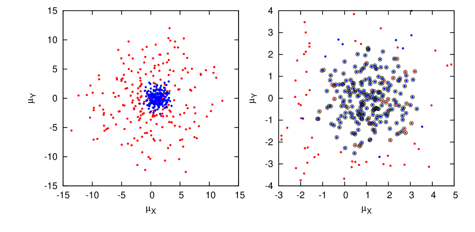
Figure 1: Proper motion for the stars of a random simulation with $N_{c,max}=N_{f,cri}=200$, $\delta=2$, and $R_{s}/R_{c}=1.1$ (see text for details of the meaning of each of these quantities). Left panel shows the distribution for all the 442 simulated stars. Red circles are the field stars centered at $(0,0)$ with $\sigma_{f}=5$ and blue circles are the $200$ cluster stars centered at $(1,0)$ with $\sigma_{c}=1$. Right panel is a magnification of the central region in which we have marked with circles the stars whose resulting cluster membership probabilities are higher than $0.5$ according to the algorithm used.

can see an example of a simulation of a cluster of $200$ stars that it has been adequately sampled with $R_{s}=1.1R_{c}$ The right panel clearly shows the occasional but inevitable “failures” of the method. First, cluster stars falling in the tails of their own distribution may not be recognized as members. Second, field stars falling by chance below the cluster distribution may be selected as probable members.

What would happen if we select a larger field? In order to address this point we have calculated membership probabilities as a function of the sampling radius. Here we are considering as cluster members those stars having membership probabilities $\geq 0.5$ in a Bayesian sense. We have done several tests by using different selection criteria and, as expected, the number of assigned members depends on it, but the main results and trends presented here remained unchanged. Figure 2 shows

Figure 2: Calculated number of field and cluster stars as a function of the sampling radius in units of the cluster radius, $R_{s}/R_{c}$, for simulations with the same set of parameters as Figure 1. (a) Simulation with peaked density profile ($\delta=0.5$), assigned members are indicated by squares connected by lines. (b) Simulation with flat density profile ($\delta=2$), members are indicated by circles connected by lines. Assigned field stars are indicated by vertical bars connected by lines, the length of the bars indicating one standard deviation. The real numbers of simulated stars are shown by dashed lines (cluster) and dotted lines (field).

the number of stars classified as members (we will denote it by $N_{c}$) or non-members ($N_{f}$) by the algorithm as a function of the sampling radius. For these particular simulations the number of assigned members $N_{c}$ is always higher than the real number of cluster stars. Most of the cluster stars are well identified but, as mentioned before, field stars falling below the cluster distribution are also considered as members. For the same reason the number of field stars is always smaller than its expected value. For $R_{s}<R_{c}$ (subsampled cluster), $N_{c}$ increases with $R_{s}$ because obviously the number of cluster stars in the sample increases as $R_{s}$ increases. The rate at which this occurs depends on the cluster density profile, that for the simulations with $\delta=2$ in Figure 2 is exacly the same as for the field (homogeneous distribution). For $R_{s}\geq R_{c}$ we observe a change in the behavior of $N_{c}$. In this case we do not include new cluster stars in the sample as $R_{s}$ increases, and $N_{c}$ increases slightly because of the new field stars that erroneously are classified as possible members. On the other hand, field stars always increase at a rate roughly proportional to $R_{s}^{2}$. It is easy to see that, in general, the fraction of cluster stars (shown in Figure 3) should

Figure 3: Calculated fraction of cluster stars as a function of the sampling radius for the same simulations as in Figure 2. The real (simulated) values are shown by dashed lines.

be a decreasing function of $R_{s}$ for any cluster with $\delta<2$. Only for the extreme case of homogeneous clusters the fraction of cluster stars remains constant with $R_{s}$ for $R_{s}<R_{c}$.

Figures 2 and 3 show the number of stars classified as members, but we do not know whether this classification is actually well done. In order to quantify the correctness of the result we define the matching fraction of the cluster $M_{c}$ as the net proportion of cluster stars that are well classified. If $N_{ok}$ is the total number of cluster stars correctly classified as members minus the number of cluster stars incorrectly classified as non-members, then $M_{c}=N_{ok}/N_{c,max}$. $M_{c}$ can be a negative number if the number of misclassifications is higher than the number of correct classifications and $M_{c}$ is exactly $1$ only when the algorithm classifies correctly all the stars of the cluster. In Figure 4 we

Figure 4: Matching fraction of the cluster (see text) as a function of the sampling radius for the same simulations as in Figure 2. The error bars are of the order of the symbol sizes but they are not shown for clarity.

see that the highest $M_{c}$ value occurs precisely when the sampling radius equals the cluster radius. At smaller sampling radii the matching fraction of the cluster obviously decreases because the cluster is being subsampled. Interestingly, the matching fraction is also smaller at $R_{s}>R_{c}$, but the reason in this case is that more field stars are being erroneously assigned to the cluster as $R_{s}$ increases. The best classification is obtained when the sampling radius is very close to the cluster radius although, as expected, even in this case the matching fraction does not reach its maximum value $M_{c}=1$. However, the matching fraction is relatively high ($M_{c}=0.83$) at $R_{s}=R_{c}$ and decreases slowly to $0.71$ at $R_{s}=1.5R_{c}$. Moreover, the behaviors of $N_{c}$ and $N_{f}$ with $R_{s}$ are very similar to the expected ones (Figures 2 and 3). This is because both cluster and field stars were simulated following perfect normal distributions and, therefore, both populations can be well detected by the algorithm since it assumes the same kind of underlying distribution. When using real data the situation becomes more complex, as discussed in the next section.

4 Results using real data

We use the CdC-SF Catalogue (Vicente et al., 2009), an astrometric catalogue with a mean precision in the proper motions of 2.0 mas/yr (1.2 mas/yr for well measured stars, typically $V<14$). Given the position of a known open cluster, we extract circular fields of varying radius centred on it and then we calculate membership probabilities by using the same algorithm as in Section 3. Here we analyze two open clusters that are included in the area covered by this catalogue: NGC 2323 (M 50) and NGC 2311. In order to minimize even more the influence of possible outliers on our results we further restrict the sample to $|\mu|\leq 20$ mas/yr. The number of probable members $N_{c}$, i.e. stars having membership probabilities higher than 0.5, is shown in Figure 5 as

Figure 5: Number of cluster stars $N_{c}$ as a function of the sampling radius $R_{s}$ in arcmin for the open clusters NGC 2323 (squares connected by lines) and NGC 2311 (circles connected by lines).

a function of the sampling radius. In general, $N_{c}$ always increases with increasing $R_{s}$ and there are no relatively flat regions analogous to those observed in Figure 2 for $R_{s}>R_{c}$. Without a previous knowledge of the approximate value of the cluster radius, how can we determine which is the most reliable result? This is not a trivial question given the large uncertainties involved in the estimation or definition of the cluster radius (see discussion in Section 4.2). For example, the radius of the total extent of NGC 2323 estimated by different authors has been varying over the last years: $10$ arcmin (Claria et al., 1998), $16.7$ arcmin (Nilakshi et al., 2002), $15$ arcmin (Kalirai et al., 2003), $22.2$ arcmin (Kharchenko et al., 2005), $17$ arcmin (Sharma et al., 2006, using their own optical data) or $22$ arcmin (Sharma et al., 2006, using 2MASS data). Our calculations yield $N_{c}=198$ probable members in a field of radius $R_{s}=17$ arcmin, but this number increases to $N_{c}=336$ for $R_{s}=22$ arcmin. This means that there could be more than $100$ undetected members if we use $R_{s}=17$ arcmin and the cluster radius is actually $R_{c}=22$ arcmin or, on the contrary, more than $100$ spurious members if we use $R_{s}=22$ arcmin and $R_{c}=17$ arcmin. The fraction of cluster members is shown in Figure 6.

Figure 6: Fraction of cluster stars as a function of the sampling radius for NGC 2323 (squares connected by lines) and NGC 2311 (circles connected by lines). Vertical arrows indicate the optimal sampling radii (see text).

The trend in which $N_{c}/(N_{c}+N_{f})$ decreases with $R_{s}$ is qualitatively consistent with the expected behavior (Figure 3). However, there is a $R_{s}$ value from which the fraction of members increases as $R_{s}$ increases and, as mentioned in the previous section, this behavior is possible only if $N_{c}$ increases faster than $N_{f}$ does (i.e. at a rate higher than $\sim R_{s}^{2}$). The only way this could happen is if the algorithm is introducing many spurious members as $R_{s}$ increases. In other words, there is a critical $R_{s}$ value above which a significant number of spurious members are erroneously included as part of the cluster (see also Piatti et al., 2009). Here we call this critical value the optimal sampling radius, $R_{s,opt}$, and obviously it is not recommended to use a sampling radius larger than this value. From Figure 6 we get $R_{s,opt}\simeq 14$ arcmin for NGC 2323 and $R_{s,opt}\simeq 13$ arcmin for NGC 2311, but we have to point out that these values are valid for the data we are using and, in principle, they cannot be extrapolated to other data sets.

The main reason behind the behavior observed in Figure 6 lies in the disagreement between the assumed and the “true” underlying distributions of proper motion of field stars. A circular normal bivariate function is a good representation of the cluster probability density function (PDF), the standard deviation being the result of observational errors that prevent the intrinsic velocity dispersion of the cluster from being completely resolved. However, it is known that an elliptical normal bivariate function is not always the best model for the field PDF (see discussions on this subject in Cabrera-Caño & Alfaro, 1990; Uribe & Brieva, 1994; Balaguer-Núñez et al., 2004; Sánchez & Alfaro, 2009; Griv et al., 2009). The combination of several factors, such as galactic differential rotation or peculiar motions, may affect the field star distribution which usually tends to exhibit non-gaussian tails. Non-parametric models, which make no a priori assumptions about the cluster or field star distributions, have been introduced and used to overcome this problem (cf. Cabrera-Caño & Alfaro, 1990; Chen et al., 1997). It is interesting to note that both the classical parametric and non-parametric methods agree reasonably well with each other only for the cases of nearly gaussian field distributions (see Figure 5 in Sánchez & Alfaro, 2009). When the number of field stars increases and the algorithm tries to fit a gaussian function to the PDF, the fit tends to produce a wider and flatter function. As a consequence, the membership probabilities (defined as the ratio of the cluster to the total proper motion distribution function) increases and therefore the number of assigned members also increases. This effect is magnified when the cluster distribution becomes “contaminated” by many field stars, because then the standard deviation of the cluster tends to increases with the consequent increasing of number of spurious members. The standard deviations estimated for the two clusters under consideration are shown in Figure 7.

Figure 7: Estimated standard deviations as a function of the sampling radius for the clusters NGC 2323 (squares connected by lines) and NGC 2311 (circles connected by lines). The bars indicate the uncertainties obtained from bootstrapping.

The error bars were estimated using bootstrap techniques: the calculation is repeated on a series of 100 random resamplings of the data and the standard deviation of the obtained set of values is taken as the associated uncertainty. The standard deviations remain nearly constant ($\sigma_{c}\simeq 1.4-1.6$ for NGC 2311 and $\sigma_{c}\simeq 0.9-1.0$ for NGC 2323) in the region in which $R_{s}\lesssim R_{s,opt}$ (see also Figure 6). This is the expected behavior because, in principle, $\sigma_{c}$ should not depend on the sample size. However, above the optimal sampling radius we can see a gradual increase in $\sigma_{c}$ due to the effect mentioned previously.

4.1 Effectiveness of membership determination

It is not possible in practice to quantify the degree of correlation between identified and true cluster members, such as the matching fraction in Figure 4. Instead, we can use the concept of effectiveness of membership determination which is set as (Tian et al., 1998; Wu et al., 2002)

$$E=1-\frac{N\sum_{i=1}^{N}\{p(i)\left[1-p(i)\right]\}}{\sum_{i=1}^{N}p(i)\sum_{i=1}^{N}\left[1-p(i)\right]}\ \ ,$$ (8)

where $p(i)$ is the membership probability of the $i$-th star and $N$ is the sample size. This index measures how effective the membership determination is in the sense of measuring the separation between field and cluster populations in the probability histogram. The higher the index $E$, the more effective the membership determination. The maximum $E$ value is obtained when there are two perfectly separated populations of $N_{c}$ stars with membership probabilities $p(i)=1$ and $N_{f}$ stars with $p(i)=0$. Figure 8

Figure 8: Effectiveness of membership determination (see Equation 8) as a function of the sampling radius for the open cluster NGC 2323 (open squares connected by solid lines) and for simulations using parameter values corresponding to those obtained for NGC 2323 (dashed lines).

shows $E$ for the open cluster NGC 2323 as a function of the sampling radius. For the sake of comparison we also show the result for simulations using the same parameters as those for NGC 2323. Our most reliable estimation for this cluster ($R_{s}=R_{s,opt}=14$ arcmin) yielded the following values for the proper motions (in mas/yr): $\mu_{x,c}=1.09$, $\mu_{y,c}=1.13$, $\sigma_{x,c}=\sigma_{y,c}=1.01$, $\mu_{x,f}=+0.77$, $\mu_{y,f}=-2.54$, $\sigma_{x,f}=6.41$, and $\sigma_{y,f}=5.84$. According to the result shown in Figure 9 (next section), we assume $R_{c}=20$ arcmin and $\delta=1.7$ for the cluster. Additionally, we choose $N_{c,max}=250$ and $N_{f,cri}=500$ in order to get the measured values $N_{c}=147$ and $N_{f}=231$ at $R_{s}=14$ arcmin. The superimposed dashed lines in Figure 8 are the average values (and their standard deviations) for these simulations. The simulated $E$ value remains fairly constant (within the uncertainties) as $R_{s}$ increases until the value $R_{s}\simeq R_{c}=20$ arcmin, beyond which it decreases at a relatively high rate. For NGC 2323 we see that $E$ begins to decrease more rapidly as $R_{s}$ increases just beyond $R_{s}\simeq R_{s,opt}=14$ arcmin. The best separations between cluster and field stars and the agreement with the simulations are achieved in the range $10\lesssim R_{s}\lesssim 14$ arcmin.

4.2 Cluster radius and optimal sampling radius

Basically what we are saying is that, at least when using only kinematical criteria, the sample size can substantially alter the results obtained (the memberships and the rest of the properties derived from there). Thus, the strategy of choosing a field large enough to be sure of covering more than the whole cluster has to be taken with extreme caution, especially in dense star fields. According to our simulations (Section 3), the best membership estimation is achieved when $R_{s}\simeq R_{c}$. This would seem an obvious result, given that for $R_{s}<R_{c}$ the cluster is subsampled whereas for $R_{s}>R_{c}$ the probability of contamination by field stars is increased. The important point here is: how well can we know the cluster radius before estimating memberships? It is difficult to determine precisely the radius of a cluster because the definition of radius is ambiguous itself, since star clusters have no well defined natural boundaries. In this work we have used the usual definition of $R_{c}$ as the radius of the circle containing all the cluster members. Most of the “geometric” definitions tend to overestimate the actual size, especially for irregularly shaped clusters (Schmeja & Klessen, 2006). But this is not the main problem. The problem is that the independent estimations of cluster radii available in the literature usually exhibit significant differences and uncertainties. Angular sizes listed in catalogues as Webda were compiled from older references (e.g. Lynga, 1987) in which most of the apparent diameters were estimated from visual inspection. According to Webda $R_{c}=7$ arcmin for NGC 2323, but in the last years this value has been triplicated (Sharma et al., 2006). As mentioned above, it is an usual practice to choose a field larger than the apparent area covered by the cluster (taken from the literature) for estimating membership probabilities. But, at least when applying the Sanders’ method, assigned members will spread throughout the whole selected area because of the contamination by field stars. It is probably not coincidental that this is the case, for example, for the probable members in the Dias catalogue (Dias et al., 2002). How reliable are all the memberships that have been derived from proper motions? It depends on the “real” $R_{c}$ values. Thus, again, the ideal situation would be some kind of robust estimation of the radius.

A commonly used procedure to determine (or define) the cluster radius is based on the analysis of the projected radial density profile. Usually, some particular analytical function (for example, a King-like model) is fitted to the density profile and the cluster radius is extracted from this fit. The last study dealing with a systematic determination of cluster sizes based on objective and uniform estimations of radial density profiles was done by Kharchenko et al. (2004). One limitation of this method is the sensitivity of the fit to small variations in the distribution of stars, especially for poorly populated open cluster. The most reliable fits are obtained using only the cluster members, but then we are confronting again the problem of membership determination. As an example, let us consider Figure 9 which

Figure 9: Radial density profiles for the cluster NGC 2323 calculated for the cases $R_{s}=14$ arcmin (solid circles) and $R_{s}=25$ arcmin (open circles). Lines show the best fits for functions of the form $\sim r^{\delta-2}$ (see Equation 6). The solid line is for the case $R_{s}=14$ arcmin for which $\delta\simeq 1.7$, and the dashed line corresponds to $R_{s}=25$ arcmin for which $\delta\simeq 1.2$.

compares the density profiles obtained for the open cluster NGC 2323 for two different sampling radii: $R_{s}=R_{s,opt}=14$ arcmin and $R_{s}=25$ arcmin. According to our results (section 4) our most reliable estimation is achieved when $R_{s}=R_{s,opt}$. For this case, the best least squares fit to a power law function suggests a cluster radius in the range $\sim 20-25$ arcmin. However, if we take a sample of size $R_{s}=25$ arcmin the contamination by field stars tends to produce an overestimation of the star density and both the index of the power law and the estimated cluster radius change notoriously (see Figure 9). But the main drawback of this method is that simple analytical fits are not always a good representation for the stars distribution in open clusters (Sánchez & Alfaro, 2009). The radius defined through a fit to a density profile may be useful in analyzing and comparing the properties of several clusters systematically, but great care must be taken when using these model-dependent definition to estimate the “true” cluster radius. In fact, the point where the fitted star density equals the background (or drops to zero) does not even necessarily agree with the outer boundary of an open cluster. In principle, new-born stars in a young cluster spread out through the region able to collapse gravitationally to form them. At certain distance from the high density peak in the molecular cloud the required conditions are not fulfilled anymore and the star formation efficiency may decrease abruptly. So, a radial star density distribution which decays smoothly to $R_{c}$ may not be always suitable, especially for compact and/or very young star clusters. Moreover, if the clusters exhibit some degree of substructure this kind of procedure yields totally unrealistic results (Sánchez & Alfaro, 2009). Young embedded clusters often show hierarchical structure (Elmegreen, 2009), so that these methods cannot in principle be applied to embedded clusters but only to centrally concentrated open clusters.

Obviously, any reliable estimation of the cluster radius ultimately depends on the membership determination. Field star contamination may affect the determination of $R_{c}$, and what we are showing in this work is that this contamination can become a severe problem if it is not taken into consideration. Furthermore, even though cluster and field populations were well separated, the estimated radius would depend on the limit magnitude if, for instance, there was mass segregation. This kind of problems is particularly relevant for the development of automated techniques in which it is necessary to establish objective criteria to decide the size of the sample to be processed. What we are proposing here is to apply any suggested method to several sample sizes $R_{s}$ and analyse the behavior obtained. It is difficult to give simple rules for evaluating this behavior because the results will depend directly on both the membership determination algorithm and the input data. However, for the method considered in this work, based on two underlying gaussian populations, the basic procedure can be outlined as follows.

1. An upper limit for $R_{s}$ can be previously estimated by fitting the spatial star density to, for example, a King profile. The estimated tidal radius (or, in order to be confident, twice its value) may be considered an upper limit of the optimal sampling radius and would define the range of $R_{s}$ values to be scanned.

2. For each $R_{s}$ value, cluster memberships and all the relevant quantities (numbers of cluster stars and field stars, centroids with their standard deviations, effectiveness of membership determination) have to be estimated.

3. The next step is to plot the number of cluster members $N_{c}$ as a function of the sampling radius $R_{s}$. If the membership determination works reasonably well, meaning that it presents little contamination by field stars, then we would observe a behavior as that seen in Figure 2: $N_{c}$ increasing as $R_{s}$ increases until some point (just when $R_{s}=R_{c}$) and then $N_{c}$ remaining approximately constant for higher $R_{s}$ values (or increasing at a much slower rate). In this way, we have a method to estimate the cluster size directly from the data and the membership criteria without making any additional assumptions. The optimal sampling radius at which we get the best membership estimation is precisely $R_{s,opt}=R_{c}$ (Fig. 4)

4. If the parametric model does not adequately describe the real data and/or if the internal noise has not a simple structure, then the behavior of the estimated parameters with $R_{s}$ would be different from the expected one. If this were the case we should plot the fraction of members $N_{c}/(N_{c}+N_{f})$ versus $R_{s}$, where we should be able to identify the optimal sampling radius $R_{s,opt}$ as the minimum in this plot (Fig 6). In absence of more accurate information, this value would correspond to the radius for which the membership classification is the most reliable (with such a method in a given astrometric catalogue).

5. Our experience indicates that the properties derived from the Sanders’ method tend to exhibit some noise and it is not always easy to identify the exact position of specific features (as the minimum in the $N_{c}/(N_{c}+N_{f})$ versus $R_{s}$ plot). Some complementary strategies may be useful in identifying or confirming the optimal sampling radius. First, one can deal with the variation of the proper motion standard deviation with radius. The dispersion of the cluster proper motions should display a change of slope at radius close to its optimal value (Fig. 7). Second, the maximum of the effectiveness of membership determination should also be around $R_{s,opt}$ (Fig.8).

The strategy proposed in this work, i.e. to estimate and analyse cluster memberships as a function of $R_{s}$, should in principle allow for the identification of the optimal sampling radius. However, we would like to emphasize that it may not always be possible (or at least not always unambiguous) to determine $R_{s,opt}$ in the way described above. For instance, for very peaked cluster density profiles the change in $N_{c}$ at $R_{s}=R_{c}$ may be not pronounced enough for being easily detected (e.g., Fig. 2a). In spite of this, it still seems appropriate and useful to perform this kind of tests before any further analysis.

5 Conclusions

We have evaluated the performance of the commonly used Sanders’ method (Vasilevskis et al., 1958; Sanders, 1971; Cabrera-Caño & Alfaro, 1985) in the determination of star cluster memberships. In general, the results depend on the radius of the field containing the sampled cluster (the sampling radius, $R_{s}$). The main reason for this dependence lies in the differences between the assumed gaussian and the true underlying proper motion distributions. The contamination of cluster members by field stars increases as the sampling radius increases. The rate at which this effect occurs depends on the intrinsic characteristics of the data set. There is a threshold value of $R_{s}$ above which the identified cluster members are highly contaminated by field stars and the effectiveness of membership determination is relatively small. Thus, care must be taken when applying the Sanders’ method (just by itself or as part of a more extensive procedure) especially when we do not have reliable information about the real cluster radius and/or when the sampling radius is larger the cluster radius. If this type of effects is not taken into consideration in automated data analysis then significant biases may arise in the derived cluster parameters. The optimal sampling radius can be estimated by plotting the number of cluster members and/or the fraction of members as a function of the sampling radius. Moreover, this type of analysis can also be used as an objective procedure that can be applied systematically to determine cluster radii.