A Classical Background for the Wave Function Prediction in the Infinite System Density Matrix Renormalization Group Method

Abstract

We report a physical background of the wave function prediction in the infinite system density matrix renormalization group (DMRG) method, from the view point of two-dimensional vertex model, a typical lattice model in statistical mechanics. Singular value decomposition applied to rectangular corner transfer matrices naturally draws matrix product representation for the maximal eigenvector of the row-to-row transfer matrix. The wave function prediction can be expressed as the insertion of an approximate half-column transfer matrix. This insertion process is in accordance with the scheme proposed by McCulloch recently.

1 Introduction

The density matrix renormalization group (DMRG) method is one of the efficient numerical method, which has been applied extensively to one-dimensional (1D) quantum systems and two-dimensional (2D) classical systems. [1, 2, 3, 4] The method is variational in the sense that it assumes a trial state, the matrix product state (MPS), which is written as a product of local tensors. [5, 6, 7, 8, 9, 10, 11, 12, 13, 14, 15] Orthogonality of each matrix ensures the numerical stability.

One of the bottleneck in the computation of the DMRG method is the diagonalization of super block Hamiltonian. The construction of a good initial vector for this diagonalization is very important. For the finite-system DMRG method, the so-called wave function renormalization scheme provides the answer. [16, 17] For the infinite-system DMRG method, Baxter’s method of corner transfer matrix (CTM), [18, 19, 20] which can be reinterpreted from the view point of the DMRG method, [21, 22] essentially solves the problem of initial vector. Based on Baxter’s CTM method, the product wave function renormalization group (PWFRG) method was proposed, [23, 24, 25] and has been applied to the study of 1D spin chains. [26, 27, 28, 29, 30, 31, 32, 33, 34, 35, 36, 37, 38, 39, 40]

Recently McCulloch proposed a way of precise wave function prediction, which works better than the PWFRG method especially when the system size is small compared with the correlation length. [41] In this paper we present a physical background for McCulloch’s scheme from the view point of 2D vertex model, one of the typical lattice model in statistical mechanics. [20] Although we employ classical lattice model, most of the obtained results can be applicable for 1D quantum systems through the quantum-classical correspondence.

Structure of the paper is as follows. In the next section we explain the symmetric vertex model, and express the maximal eigenstate of the row-to-row transfer matrix by use of CTMs. In §3 we consider the area extension of CTMs, introducing an approximate half-column transfer matrix. We show the connection between MPS and CTM formulation in §4, where the system size extension scheme by McCulloch is obtained naturally. We summarize the obtained result in the last section, and discuss the remaining problem on the MPS obtained by the finite-system DMRG method.

2 Eigenstate of row-to-row Transfer Matrix Approximated by Corner Transfer Matrices

Figure 1: A finite size vertex model of width $N=8$. Cross marks show boundary spins and open circles show row spins, which are the variables of $\Psi_{8}^{~{}}$ in Eq. (2.1). The system consists of its left-half and the right half, where the vertical stitch corresponds to the half-column spin $\sigma_{1}^{~{}},\sigma_{2}^{~{}},\sigma_{3}^{~{}},\ldots$ between them.

Throughout this article we consider a square-lattice symmetric vertex model, [20] as an example of 2D classical lattice models. There is a $d$-state spin variable on each bond, which connects neighboring lattice points. Four spins around a lattice point determine the local Boltzmann weight $W$, which is called as the vertex weight. We assume that the vertex weight is position independent, and therefore the system is uniform. We also assume that each vertex weight is invariant under exchange of left and right spin variables, and those of up and down spin variables. In other words, we consider the symmetric vertex model in order to simplify the following formulation.

As shown on the left side of Fig. 1, we treat a finite size system that has a rectangular shape. This system corresponds to the stack of row-to-row transfer matrices $T_{N}^{~{}}$, whose width is $N$, multiplied by an initial vector $V_{N}^{~{}}$. We choose $V_{N}^{~{}}$ so that it corresponds to the boundary condition at the bottom of the system, where there is a row of boundary spins shown by the cross marks. Those cross marks aligned vertically also represent boundary spins, that are located at the both ends of $T_{N}^{~{}}$. The row of open circles represents spins on top of the rectangular system. We consider a $d^{N}_{~{}}$-dimensional vector

$$\Psi_{N}^{~{}}=T_{N}^{~{}}T_{N}^{~{}}T_{N}^{~{}}\ldots T_{N}^{~{}}V_{N}^{~{}}\,,$$ (1)

where the number of the row-to-row transfer matrix $T_{N}^{~{}}$ is sufficiently large. Under this assumption we can expect that $\Psi_{N}^{~{}}$ is a good approximation of the maximal eigenvector of $T_{N}^{~{}}$ if $V_{N}^{~{}}$ is not orthogonal to that.

For a while let us consider the case $N=8$; generalization to arbitrary $N$ is straightforward. We label the top spins as $q_{1}^{~{}},\,q_{2}^{~{}},\,q_{3}^{~{}},\,q_{4}^{~{}},\,p_{4}^{~{}},\,p_{3}^{~{}},\,p_{2}^{~{}}$, and $p_{1}^{~{}}$ from left to right. The vector elements of $\Psi_{8}^{~{}}$ are then written as $\Psi_{8}^{~{}}(q_{1}^{~{}},\,q_{2}^{~{}},\,q_{3}^{~{}},\,q_{4}^{~{}},\,p_{4}^{~{}},\,p_{3}^{~{}},\,p_{2}^{~{}},\,p_{1}^{~{}})$. Since we have assumed the left-right symmetry for the vertex weight, it is convenient to divide the row-spin into the left half $q_{1}^{~{}},\,q_{2}^{~{}},\,q_{3}^{~{}},\,q_{4}^{~{}}$, where we have counted them from left to right, and the right half $p_{1}^{~{}},\,p_{2}^{~{}},\,p_{3}^{~{}},\,p_{4}^{~{}}$, where we have counted them from right to left. (See right bottom of Fig. 1.) According to this division, we can interpret $\Psi_{8}^{~{}}$ as a $d^{4}_{~{}}$-dimensional real symmetric matrix, whose elements can be expressed as $\Psi_{8}^{~{}}(q_{1}^{~{}}\,q_{2}^{~{}}\,q_{3}^{~{}}\,q_{4}^{~{}}|p_{1}^{~{}}\,p_{2}^{~{}}\,p_{3}^{~{}}\,p_{4}^{~{}})$. We have used the vertical bar “$|$” to separate the left and the right indices, and dropped the commas between the spin variables for the book keeping. If necessary, we further abbreviate the matrix notation as $\Psi_{8}^{~{}}(q|p)$.

We express the left half of the rectangular system by use of the CTM, whose elements are written as $C_{4}^{~{}}(q_{1}^{~{}}\,q_{2}^{~{}}\,q_{3}^{~{}}\,q_{4}^{~{}}|\sigma_{1}^{~{}}\,\sigma_{2}^{~{}}\,\sigma_{3}^{~{}}\,\ldots)$, where $\sigma_{1}^{~{}}\,\sigma_{2}^{~{}}\,\sigma_{3}^{~{}}\,\ldots$ represent the half-column spins at the center of the system. In the same manner we can express the right half by the transpose of $C_{4}^{~{}}$, i.e., $C_{4}^{~{}T}$. Joining process of these halves by stitching $C_{4}^{~{}}$ and $C_{4}^{~{}T}$ via the contraction of the half-column spins can be expressed simply by the product of matrices $\Psi_{8}^{~{}}=C_{4}^{~{}}\,C_{4}^{~{}T}$. More precisely, there is a relation

$$\Psi_{8}^{~{}}(q|p)=\sum_{\sigma}^{~{}}C_{4}^{~{}}(q|\sigma)\,C_{4}^{~{}}(p|\sigma)\,,$$ (2)

where we have used the abbreviations $q=q_{1}^{~{}}\,q_{2}^{~{}}\,q_{3}^{~{}}\,q_{4}^{~{}}$, $\,p=p_{1}^{~{}}\,p_{2}^{~{}}\,p_{3}^{~{}}\,p_{4}^{~{}}$, and $\sigma=\sigma_{1}^{~{}}\sigma_{2}^{~{}}\sigma_{3}^{~{}}\ldots\,\,\,$. Since we have assumed that the number of $T_{8}^{~{}}$ in Eq. (2.1) is sufficiently large, the same for the number of column-spin $\sigma$. Although we treat $\sigma$, we do not think of them as spins directly treated in numerical calculations, unlike $q$ and $p$.

Figure 2: The singular value decomposition applied to $C_{4}^{~{}}$. The black square and circle corresponds to the block spin $\xi$ and the singular values $\Omega_{4}^{~{}}(\xi)$, respectively. The left and the right triangles represent $A_{4}^{~{}}$ and $U_{4}^{~{}}$, respectively.

One of the fundamental mathematical tool in the DMRG method is the singular value decomposition (SVD). [1, 2] Let us apply it to the CTM

$$C_{4}^{~{}}(q|p)=\sum_{\xi}^{~{}}A_{4}^{~{}}(q|\xi)\,\Omega_{4}^{~{}}(\xi)\,U_{4}^{~{}}(\sigma|\xi)\,,$$ (3)

where $\xi$ is a $d^{4}_{~{}}$-state block-spin (or an auxiliary) variable, and $\Omega_{4}^{~{}}(\xi)$ represents the singular values. The matrix $A_{4}^{~{}}$ is $d^{4}_{~{}}$-dimensional, and it satisfies the orthogonal relations

$$\sum_{\xi}^{~{}}A_{4}^{~{}}(q^{\prime}|\xi)\,A_{4}^{~{}}(q|\xi)\!\!\! = \!\!\!\delta(q^{\prime}|q)\,,$$

$$\sum_{q}^{~{}}A_{4}^{~{}}(q|\xi^{\prime})\,A_{4}^{~{}}(q|\xi)\!\!\! = \!\!\!\delta(\xi^{\prime}|\xi)\,,$$ (4)

where $\delta(\xi^{\prime}|\xi)$ is Kronecker’s delta, and where $\delta(q^{\prime}|q)$ is defined as

$$\delta(q^{\prime}|q)=\prod_{i=1}^{4}\delta(q^{\prime}_{i}|q_{i}^{~{}})\,.$$ (5)

The above orthogonal relation can be written shortly as $A_{4}^{~{}}A_{4}^{~{}T}=A_{4}^{~{}T}A_{4}^{~{}}=I_{4}^{~{}}$. Column vectors of the rectangular matrix $U_{4}^{~{}}$ are also orthogonal with each other,

$$\sum_{\sigma}^{~{}}U_{4}^{~{}}(\sigma|\xi^{\prime})\,U_{4}^{~{}}(\sigma|\xi)=\delta(\xi^{\prime}|\xi)\,,$$ (6)

but the row vectors are not

$$\sum_{\xi}^{~{}}U_{4}^{~{}}(\sigma^{\prime}|\xi)\,U_{4}^{~{}}(\sigma|\xi)\neq\delta(\sigma^{\prime}|\sigma)\,.$$ (7)

This is because the degree of freedom of $\sigma$ is far larger than that of $q$ or $\xi$. Figure 2 is the pictorial representation of SVD applied to $C_{4}^{~{}}$.

We often regard the singular values $\Omega_{4}^{~{}}$ as the diagonal matrix $\Omega_{4}^{~{}}(\xi^{\prime}|\xi)=\Omega_{4}^{~{}}(\xi)\,\delta(\xi^{\prime}|\xi)$, and write Eq. (2.3) shortly as $C_{4}^{~{}}=A_{4}^{~{}}\,\Omega_{4}^{~{}}\,U_{4}^{~{}T}$. For the latter convenience, let us introduce the generalized inverse of the CTM

$$C_{4}^{-1}=U_{4}^{~{}}\,\Omega_{4}^{-1}A_{4}^{~{}T}\,,$$ (8)

which satisfies the relation

$$C_{4}^{~{}}\,C_{4}^{-1}\!\!\! = \!\!\!A_{4}^{~{}}\,\Omega_{4}^{~{}}\,U_{4}^{~{}T}U_{4}^{~{}}\,\Omega_{4}^{-1}A_{4}^{~{}T}$$ (9)

$$= \!\!\!A_{4}^{~{}}\,A_{4}^{~{}T}=I_{4}^{~{}}\,.$$

It should be noted that $C_{4}^{-1}C_{4}^{~{}}$ is a projection operator

$$U_{4}^{~{}}\,\Omega_{4}^{-1}A_{4}^{~{}T}A_{4}^{~{}}\,\Omega_{4}^{~{}}\,U_{4}^{~{}T}=U_{4}^{~{}}\,U_{4}^{~{}T}$$ (10)

in the left hand side of Eq. (2.7), where $(C_{4}^{-1}C_{4}^{~{}})^{2}_{~{}}=C_{4}^{-1}C_{4}^{~{}}$ holds.

In the context of the DMRG method, small singular values are neglected when it is impossible to store matrix elements during the numerical calculation. This truncation is a kind of decimation in the renormalization group (RG) theory. Under the truncation, the matrices $A_{4}^{~{}}$ work as the RG transformation that controls numerical precision. In the next section we do not truncate singular values, in order to avoid complications in notations, and the introduction of truncation is straightforward.

3 Half Column Transfer Matrix and Matrix Product State

Figure 3: The pictorial representation of $P_{4}^{~{}}=C_{3}^{-1}\!\cdot C_{4}^{~{}}$ in Eq. (3.1). The circle with the cross mark shows $\Omega_{3}^{-1}$. Since $P_{4}^{~{}}$ has a function of extending the area of CTM, it can be regarded as an approximation for the half-column transfer matrix.

We introduce a new notation between matrices, the dot product, which contract variables according to Einstein rule. As an example, let us consider

$$P_{4}^{~{}}=C_{3}^{-1}\!\cdot C_{4}^{~{}}\,,$$ (11)

where $q_{1}^{~{}}$, $q_{2}^{~{}}$, and $q_{3}^{~{}}$ are contracted but $q_{4}^{~{}}$ is not, since the first three spins are shared by $C_{3}^{-1}$ and $C_{4}^{~{}}$. Figure 3 shows this rule graphically. Substituting Eq. (2.3) and (2.8) to $C_{3}^{-1}\!\cdot C_{4}^{~{}}$, we obtain

$$P_{4}^{~{}} = (U_{3}^{~{}}\,\Omega_{3}^{-1}A_{3}^{~{}T})\cdot(A_{4}^{~{}}\,\Omega_{4}^{~{}}\,U_{4}^{~{}T})$$ (12)

$$= U_{3}^{~{}}\,\Omega_{3}^{-1}\!\cdot(A_{3}^{~{}T}\!\cdot A_{4}^{~{}})\,\Omega_{4}^{~{}}\,U_{4}^{~{}T}$$

$$= U_{3}^{~{}}\,\Omega_{3}^{-1}\!\cdot{\tilde{A}}_{4}^{~{}}\,\Omega_{4}^{~{}}\,U_{4}^{~{}T}\,.$$

To avoid any confusion, let us write down element of $P_{4}^{~{}}$

$$P_{4}^{~{}}(\sigma^{\prime}|q_{4}^{~{}}|\sigma)$$ (13)

$$=\sum_{\xi\zeta}^{~{}}U_{3}^{~{}}(\sigma^{\prime}|\xi)\,\Omega_{3}^{-1}(\xi)\,{\tilde{A}}_{4}^{~{}}(\xi\,q_{4}^{~{}}|\zeta)\,\Omega_{4}^{~{}}(\zeta)\,U_{4}^{~{}}(\sigma|\zeta)\,,$$

where the new matrix ${\tilde{A}}_{4}^{~{}}=A_{3}^{~{}T}\!\cdot A_{4}^{~{}}$ is the renormalized orthogonal matrix

$${\tilde{A}}_{4}^{~{}}(\xi\,q_{4}^{~{}}|\zeta)=\sum_{q_{1}^{~{}}\,q_{2}^{~{}}\,q_{3}^{~{}}}^{~{}}A_{3}^{~{}}(q_{1}^{~{}}\,q_{2}^{~{}}\,q_{3}^{~{}}|\xi)\,A_{4}^{~{}}(q_{1}^{~{}}\,q_{2}^{~{}}\,q_{3}^{~{}}\,q_{4}^{~{}}|\zeta)\,,$$ (14)

which satisfies the relation

$$\sum_{\xi q_{4}}^{~{}}{\tilde{A}}_{4}^{~{}}(\xi\,q_{4}^{~{}}|\zeta^{\prime})\,{\tilde{A}}_{4}^{~{}}(\xi\,q_{4}^{~{}}|\zeta)=\delta(\zeta^{\prime}|\zeta)\,.$$ (15)

In Eq. (3.4) the group of spins $q_{1}^{~{}}$, $q_{2}^{~{}}$, and $q_{3}^{~{}}$ are mapped onto the block spin $\xi$ by the RG transformation $A_{3}^{~{}}$. The obtained ${\tilde{A}}_{4}^{~{}}$ corresponds to the matrix that constructs MPS, which is constructed by the infinite system DMRG method, as shown later.

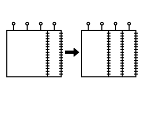
Figure 4: The area of CTM can be extended by applying the approximate half-column transfer matrices.

The $P_{4}$ thus obtained has a function of half-column transfer matrix (HCTM), since it extends the width of $C_{3}^{~{}}$ by one by way of the dot product

$$C_{3}^{~{}}\cdot P_{4}^{~{}}=C_{3}^{~{}}\cdot(C_{3}^{-1}\!\cdot C_{4}^{~{}})=(C_{3}^{~{}}\,C_{3}^{-1})\cdot C_{4}^{~{}}=C_{4}^{~{}}$$ (16)

as shown in the left side of Fig. 4. Applying SVD to $C_{3}^{~{}}$ and substituting Eq. (3.2), $C_{3}^{~{}}\cdot P_{4}^{~{}}$ is calculated as

$$(A_{3}^{~{}}\,\Omega_{3}^{~{}}\,U_{3}^{~{}T})\cdot(U_{3}^{~{}}\,\Omega_{3}^{-1}\!\cdot{\tilde{A}}_{4}^{~{}}\,\Omega_{4}^{~{}}\,U_{4}^{~{}T})=A_{3}^{~{}}\cdot{\tilde{A}}_{4}^{~{}}\,\Omega_{4}^{~{}}\,U_{4}^{~{}T}\,.$$ (17)

Since $C_{3}^{~{}}$ is again constructed from $C_{2}^{~{}}$ and $P_{3}^{~{}}$, as shown in the right side of Fig. 4, we can further decompose $C_{4}^{~{}}$ as

$$C_{4}^{~{}}=C_{2}^{~{}}\!\cdot\!P_{3}^{~{}}\!\cdot\!P_{4}^{~{}}=A_{2}^{~{}}\!\cdot\!{\tilde{A}}_{3}^{~{}}\!\cdot\!{\tilde{A}}_{4}^{~{}}\,\Omega_{4}^{~{}}\,U_{4}^{~{}T}\,.$$ (18)

The contraction process by the dot products are shown in the right side of Fig. 5. It should be noted that $C_{2}^{~{}}\cdot P_{4}^{~{}}$ is not $C_{3}^{~{}}$, since $U_{2}^{~{}T}$ contained in $C_{2}^{~{}}$ and $U_{3}^{~{}}$ contained in $P_{4}^{~{}}$ do not matches to give an identity. In this sense, $P_{4}^{~{}}$ is an approximation for the half column transfer matrix, optimized for the area extension of $C_{3}^{~{}}$ only.

Figure 5: Pictorial representation of Eq. (3.8).

Using the decomposition of $C_{4}^{~{}}$ in Eq. (3.8), we obtain the matrix product representation of $\Psi_{8}^{~{}}=C_{4}^{~{}}C_{4}^{~{}T}$. We have

$$\Psi_{8}^{~{}} = A_{2}^{~{}}\!\cdot\!{\tilde{A}}_{3}^{~{}}\!\cdot\!{\tilde{A}}_{4}^{~{}}\,(\Omega_{4}^{~{}})^{2}_{~{}}{\tilde{A}}_{4}^{~{}T}\!\!\cdot\!{\tilde{A}}_{3}^{~{}T}\!\!\cdot\!A_{2}^{~{}T}$$ (19)

$$= A_{2}^{~{}}\!\cdot\!{\tilde{A}}_{3}^{~{}}\!\cdot\!{\tilde{A}}_{4}^{~{}}\,\Lambda_{4}^{~{}}\,{\tilde{A}}_{4}^{~{}T}\!\!\cdot\!{\tilde{A}}_{3}^{~{}T}\!\!\cdot\!A_{2}^{~{}T}\,,$$

where $\Lambda_{4}^{~{}}=(\Omega_{4}^{~{}})^{2}_{~{}}$ is the singular value of $\Psi_{8}^{~{}}$. (See Fig. 6.) Such a construction of $\Psi_{8}^{~{}}$ is equivalent to the MPS considered in the context of the infinite system DMRG method.

Figure 6: Matrix product expression of $\Psi_{8}^{~{}}$ in Eq. (3.9). Double circle represent $\Lambda_{4}^{~{}}=(\Omega_{4}^{~{}})^{2}_{~{}}$.

4 Approximate Area Extension

Figure 7: Approximate area extension process $C_{5}^{App.}=C_{4}^{~{}}\cdot{\bar{P}}_{4}^{~{}}$.

Let us consider a problem of obtaining an approximation of $C_{5}^{~{}}=C_{4}^{~{}}\cdot P_{5}^{~{}}$ without using $P_{5}^{~{}}$. This attempt is equivalent to construct an approximation for $C_{5}^{~{}}$ using $C_{2}^{~{}}$, $C_{3}^{~{}}$, or $C_{4}^{~{}}$. One might think that $P_{4}^{~{}}=C_{3}^{-1}\cdot C_{4}^{~{}}=U_{3}^{~{}}\,\Omega_{3}^{-1}\!\cdot{\tilde{A}}_{4}^{~{}}\,\Omega_{4}^{~{}}\,U_{4}^{~{}T}$ can be of use as an approximation for $P_{5}^{~{}}$. But this idea should be rejected since $U_{4}^{~{}T}U_{3}^{~{}}$, which appears in the calculation of $C_{4}^{~{}}\cdot P_{4}^{~{}}$, is not an identity. A way to avoid this mismatching is to introduce a spatial reflection of $P_{4}^{~{}}$, which is defined as

$${\bar{P}}_{4}^{~{}}=U_{4}^{~{}}\,\Omega_{4}^{~{}}\,{\tilde{A}}_{4}^{~{}T}\!\cdot\Omega_{3}^{-1}U_{3}^{~{}T}\,,$$ (20)

and use it as an approximation for $P_{5}^{~{}}$. Leaving the validity of the approximation scheme by the latter discussion, let us calculate the approximate extension $C_{5}^{App.}=C_{4}^{~{}}\cdot{\bar{P}}_{4}^{~{}}$ and write it into the matrix product representation. (See Fig. 7.) We obtain

$$C_{5}^{App.} = A_{2}^{~{}}\!\cdot\!{\tilde{A}}_{3}^{~{}}\!\cdot\!{\tilde{A}}_{4}^{~{}}\,\Omega_{4}^{~{}}\,U_{4}^{~{}T}\,\,\,U_{4}^{~{}}\,\Omega_{4}^{~{}}\,{\tilde{A}}_{4}^{~{}T}\!\cdot\Omega_{3}^{-1}U_{3}^{~{}T}$$ (21)

$$= A_{2}^{~{}}\!\cdot\!{\tilde{A}}_{3}^{~{}}\!\cdot\!{\tilde{A}}_{4}^{~{}}\,(\Omega_{4}^{~{}})^{2}_{~{}}{\tilde{A}}_{4}^{~{}T}\!\cdot\Omega_{3}^{-1}U_{3}^{~{}T}$$

$$= A_{2}^{~{}}\!\cdot\!{\tilde{A}}_{3}^{~{}}\!\cdot\!{\tilde{A}}_{4}^{~{}}\,\Lambda_{4}^{~{}}\,{\tilde{A}}_{4}^{~{}T}\!\cdot\Omega_{3}^{-1}U_{3}^{~{}T}\,,$$

and from this approximation we can construct

$$\Psi_{10}^{App.} = C_{5}^{App.}(C_{5}^{App.})^{T}_{~{}}$$

$$= A_{2}^{~{}}\!\cdot\!{\tilde{A}}_{3}^{~{}}\!\cdot\!{\tilde{A}}_{4}^{~{}}\,\Lambda_{4}^{~{}}\,{\tilde{A}}_{4}^{~{}T}\!\cdot\Lambda_{3}^{-1}\!\cdot\!{\tilde{A}}_{4}^{~{}}\,\Lambda_{4}^{~{}}\,{\tilde{A}}_{4}^{~{}T}\!\cdot\!{\tilde{A}}_{3}^{~{}T}\!\cdot\!A_{2}^{~{}T}\,,$$

which may approximate $\Psi_{10}^{~{}}$. Applying Schmidt orthogonalization for $\Lambda_{4}^{~{}}{\tilde{A}}_{4}^{~{}T}$ from the left side

$$\Lambda_{4}^{~{}}\,{\tilde{A}}_{4}^{~{}T}={\tilde{B}}\,\Lambda$$ (23)

we obtain the new orthogonal matrix ${\tilde{B}}$ and the right triangular matrix $\Lambda$. (See Fig. 8.) Substituting Eq. (4.4) into Eq. (4.3), we get the matrix product expression

$$\Psi_{10}^{App.}=A_{2}^{~{}}\!\cdot\!{\tilde{A}}_{3}^{~{}}\!\cdot\!{\tilde{A}}_{4}^{~{}}\!\cdot\!{\tilde{B}}\,\Lambda\,\Lambda_{3}^{-1}\Lambda_{~{}}^{\,T}\,{\tilde{B}}_{~{}}^{\,T}\!\cdot\!{\tilde{A}}_{4}^{~{}T}\!\cdot\!{\tilde{A}}_{3}^{~{}T}\!\cdot\!A_{2}^{~{}T}\,.$$ (24)

The extension from $\Psi_{8}^{~{}}$ to $\Psi_{10}^{App.}$ is the same as the wave function extension scheme proposed by McCulloch, [41] where the approximation for the renormalized wave function is given by

$${\tilde{\Psi}}_{10}^{App.}={\tilde{B}}\,\Lambda\,\Lambda_{3}^{-1}\Lambda_{~{}}^{\,T}\,{\tilde{B}}_{~{}}^{\,T}\,.$$ (25)

Figure 8: Reorthogonalization process in Eq. (4.3). The rectangular in the lower diagram corresponds to $\Lambda$ in Eq. (4.4).

We have thus obtained a natural explanations for McCulloch’s extension scheme from the view point of 2D vertex model. Up to now we have not considered the effect of basis truncation, which is used in numerical calculation of the infinite system DMRG method. First of all, the extension in Eqs. (4.4) and (4.5) is still efficient under the truncation, as it was shown numerically. [41] We then consider the extension from $\Psi_{N}^{~{}}$ to ${\tilde{\Psi}}_{N+2}^{~{}}$ in the large system size limit $N\rightarrow\infty$. For simplicity, let us assume that the MPS in this limit is uniform, and the system is away from criticality. In this limit we can drop the site index from Eq. (4.1), and can express the approximate transfer matrix as

$$P=U\,\Omega_{~{}}^{-1}\!\cdot{\tilde{A}}\,\Omega\,U_{~{}}^{\,T}=U\!\cdot\!{\tilde{S}}\,U_{~{}}^{\,T}\,,$$ (26)

where ${\tilde{S}}=\Omega_{~{}}^{-1}\!\cdot{\tilde{A}}\,\Omega$. From the assumed symmetry of the vertex model, both $P$ and ${\tilde{S}}$ are symmetric

$$P(\sigma^{\prime}|\,q\,|\sigma) = P(\sigma|\,q\,|\sigma^{\prime})$$

$${\tilde{S}}(\sigma^{\prime}|\,q\,|\sigma) = {\tilde{S}}(\sigma|\,q\,|\sigma^{\prime})\,.$$ (27)

This symmetry is also expressed in short form as ${\bar{P}}=P$ and ${\bar{\tilde{S}}}={\tilde{S}}$. Thus at least when the system size $N=2i$ is large enough, typically several times larger than the correlation length, one can justify the usage of $C_{i}^{~{}}\cdot{\bar{P}}_{i}^{~{}}$ as the approximation for $C_{i}^{~{}}\cdot P_{i+1}^{~{}}$.

Before closing this section, we consider the MPS expression for $\Psi_{N}^{~{}}$ that is optimized by way of the sweeping process in the finite system DMRG method. The matrix product structure

$$\Psi_{N}^{~{}}=A_{2}^{~{}}\!\cdot\!{\tilde{A}}_{3}^{~{}}\!\cdots\!{\tilde{A}}_{\frac{N}{2}}^{~{}}\,\Lambda_{\frac{N}{2}}^{~{}}\,{\tilde{A}}_{\frac{N}{2}}^{~{}T}\!\!\cdots\!{\tilde{A}}_{3}^{~{}T}\!\!\cdot\!A_{2}^{~{}T}$$ (28)

is similar to that obtained by the infinite system DMRG method, but in this case the matrices satisfies the additional relation

$${\tilde{A}}_{i}^{~{}}\Lambda_{i}^{~{}}=\Lambda_{i-1}^{~{}}{\tilde{A}}_{i}^{~{}T}\,,$$ (29)

where both ${\tilde{A}}_{i}^{~{}}$ and $\Lambda_{i}^{~{}}$ differ from those obtained by the infinite system DMRG method. Taking the square root of $\Lambda_{i}^{~{}}$, we formally obtain a diagonal matrix $\Omega_{i}^{~{}}=\sqrt{\Lambda_{i}^{~{}}}$. It should be noted that this $\Omega_{i}^{~{}}$ is different from that obtained from the SVD applied to $C_{i}^{~{}}$. Defining

$${\tilde{S}}_{i}^{~{}}=\Omega_{i-1}^{-1}\!\cdot\!{\tilde{A}}_{i}^{~{}}\,\Omega_{i}^{~{}}=\Omega_{i-1}^{~{}}{\tilde{A}}_{i}^{~{}T}\!\cdot\Omega_{i}^{-1}$$ (30)

and substituting it to Eq. (4.9), we obtain a new standard form for MPS

$$\Psi_{N}^{~{}}=\Omega_{1}^{~{}}\,S_{2}^{~{}}\!\cdot\!{\tilde{S}}_{3}^{~{}}\!\cdots\!{\tilde{S}}_{\frac{N}{2}}^{~{}}\,{\tilde{S}}_{\frac{N}{2}}^{~{}T}\!\!\cdots\!{\tilde{S}}_{3}^{~{}T}\!\!\cdot\!S_{2}^{~{}T}\,\Omega_{1}^{~{}}\,,$$ (31)

where $\Omega_{1}^{~{}}$ is just a constant and is not essential. It is then straightforward to obtain the approximation $\Psi_{N+2}^{App.}$ just by putting ${\bar{\tilde{S}}}_{\frac{N}{2}}^{~{}}\,{\bar{\tilde{S}}}_{\frac{N}{2}}^{~{}T}$ at the center of the above MPS, where this insertion is a variant of Eq. (4.5). In the thermodynamic limit $N\rightarrow\infty$ the matrix ${\tilde{S}}_{i}^{~{}}$ in Eq. (4.11) is independent on the site index $i$, and therefore it coincides with ${\tilde{S}}$ in Eq. (4.8). This symmetric representation of uniform MPS is often of use.

Figure 9: Graphical representation of Eq. (4$\cdot$14).

5 Conclusions and Discussions

We have considered the wave function prediction in the infinite system DMRG method, when it is applied to the 2D vertex model. Through the singular value decomposition of CTM $C_{i}^{~{}}$, we obtained the approximate half-column transfer matrix $P_{i}^{~{}}$. The insertion of ${\bar{P}}_{i}^{~{}}$ naturally explains the wave function prediction proposed by McCulloch, [41] which works better than the product wave function renormalization group (PWFRG) method, [23, 24, 25] especially when the system size is small. The difference between these two prediction methods can be explained by the shape of finite size system. The PWFRG method treats growing triangular cluster, [24] whereas McCulloch’s scheme always treat half-infinite stripe.

The relation between CTM and MPS in the finite-system DMRG method is not so clear. For example, $\Psi_{8}^{~{}}$ can be expressed as $C_{3}^{~{}}\,C_{5}^{~{}T}$, but the MPS representation of the optimized $\Psi_{8}^{~{}}$ by the finite system DMRG cannot be obtained from the SVD applied to $C_{3}^{~{}}$ and $C_{5}^{~{}}$ independently. This puzzle is something to do with the targeting scheme for asymmetric vertex model, and also with the determination of optimal RG transformation in the real-time DMRG method, where the density matrix is time dependent.

References

[1] S. R. White: Phys. Rev. Lett. 69 (1992) 2863;
Phys. Rev. B 48 (1993) 10345.
[2]Density-Matrix Renormalization
- A New Numerical Method in Physics -, eds.
I. Peschel, X. Wang, M. Kaulke, and K. Hallberg (Springer, Berlin, 1999)
and references therein.
[3] T. Nishino, T. Hikihara, K. Okunishi, and Y. Hieida: Int. J. Mod.
Phys. B 13 (1999) 1.
[4] U. Schollwöck: Rev. Mod. Phys. 77 (2005) 259.
[5] I. Affleck, T. Kennedy, E. H. Lieb, and H. Tasaki: Phys.
Rev. Lett. 59 (1987) 799.
[6] M. Fannes, B. Nachtergale, and R. F. Werner: Europhys. Lett.
10 (1989) 633.
[7] M. Fannes, B. Nachtergale, and R. F. Werner: Commun. Math.
Phys. 144 (1992) 443.
[8] M. Fannes, B. Nachtergale, and R. F. Werner: Commun. Math. Phys. 174 (1995) 477.
[9] A. Klümper, A. Schadschneider, and J. Zittartz:
Z. Phys. B 87 (1992) 281.
[10] H. Niggemann, A. Klümper, and J. Zittartz:
Z. Phys. B 104 (1997) 103.
[11] S. Östlund and S. Rommer: Phys. Rev. Lett 75 (1995) 3537.
[12] S. Rommer and S. Östlund: Phys. Rev. B 55 (1997) 2164.
[13] M. Andersson, M. Boman, and S. Östlund: Phys. Rev. B 59 (1999) 10493.
[14] H. Takasaki, T. Hikihara, and T. Nishino: J. Phys. Soc. Jpn. 68 (1999) 1537.
[15] J. Dukelsky, M. A. Martín-Delgado, T. Nishino, and G. Sierra:
Europhys. Lett. 43 (1998) 457.
[16] S. R. White and I. Affleck: Phys. Rev. B 54 (1996) 9862.
[17] S. R. White: Phys Rev Lett. 77 (1996) 3633.
[18] R. J. Baxter: J. Math. Phys 9 (1968) 650.
[19] R. J. Baxter: J. Stat. Phys. 19 (1978) 461.
[20] R. J. Baxter: Exactly Solved Models in Statistical
Mechanics (Academic Press, London, 1982).
[21] T. Nishino and K. Okunishi: J. Phys. Soc. Jpn. 65 (1996) 891.
[22] T. Nishino and K. Okunishi: J. Phys. Soc. Jpn. 66 (1997) 3040.
[23] T. Nishino and K. Okunishi: J. Phys. Soc. Jpn. 64 (1995) 4084.
[24] K. Ueda, T. Nishino, K Okunishi, Y. Hieida, R. Derian, and A. Gendiar:
J. Phys. Soc. Jpn. 75 (2006) 014003.
[25] H. Ueda, T. Nishino, K. Kusakabe:
J. Phys. Soc. Jpn. 77 (2008) 114002.
[26] N. Akutsu and Y. Akutsu: Phys. Rev. B 57 (1998) R4233.
[27]
N. Akutsu and Y. Akutsu: Prog. Theor. Phys. 105 (2001) 123.
[28]
N. Akutsu, Y. Akutsu, and T. Yamamoto: Prog. Theor. Phys. 105 (2001) 361.
[29]
N. Akutsu, Y. Akutsu, and T. Yamamoto: Phys. Rev. B 64 (2001) 085415.
[30]
N. Akutsu, Y. Akutsu, and T. Yamamoto: J. of Cryst. Growth 237-239 (2002) 14.
[31]
N. Akutsu, Y. Akutsu, and T. Yamamoto: Phys. Rev. B 67 (2003) 125407.
[32] Y. Hieida, K. Okunishi, and Y. Akutsu:
Phys. Lett. A 233 (1997) 464.
[33]
M. Hagiwara, Y. Narumi, K. Kindo, M. Kohno, H. Nakano, R. Sato, and M. Takahashi:
Phys. Rev. Lett. 80 (1998) 1312.
[34] K. Okunishi, Y. Hieida, and Y. Akutsu: Phys. Rev. B 59
(1999) 6806.
[35]
K. Okunishi, Y. Hieida, and Y. Akutsu
Phys. Rev. E 59 (1999) R6227.
[36]
Y. Hieida, K. Okunishi, and Y. Akutsu:
New J. of Phys. 1 (1999) 7.1.
[37]
K. Okunishi, Y. Hieida, and Y. Akutsu:
Phys. Rev. B 60 (1999) R6953.
[38]
Y. Hieida, K. Okunishi, and Y. Akutsu:
Phys. Rev. B 64 (2001) 224422.
[39] Y. Narumi, K. Kindo, M. Hagiwara, H. Nakano, A. Kawaguchi,
K. Okunishi, and M. Kohno:
Phys. Rev. B 69 (2004) 174405.
[40] S. Yoshikawa, K. Okunishi, M. Senda, and S. Miyashita:
J. Phys. Soc. Jpn. 73 (2004) 1798.