Approximating Partition Functions of Two-State Spin Systems

Abstract

Two-state spin systems is a classical topic in statistical physics. We consider the problem of computing the partition function of the systems on a bounded degree graph. Based on the self-avoiding tree, we prove the systems exhibits strong correlation decay under the condition that the absolute value of “inverse temperature” is small. Due to strong correlation decay property, an FPTAS for the partition function is presented under the same condition. This condition is sharp for Ising model.


Keywords: Strong correlation decay; Self-avoiding tree; Ising model; FPTAS; Partition function


1. Introduction

Spin model with $p$ states is a classical mathematical model in statistical physics. Such models describe and explain the behavior of ferromagnets, lattice gas and certain other phenomena of statistical physics. In this paper, we focus on the case of two spins. This case encompasses models of physical interest, such as the classical Ising model (ferromagnetic or antiferromagnetic, with or without an applied magnetic field).

In statistical mechanics, the partition function is an important quantity that encodes the statistical properties of a system in thermodynamic equilibrium. However, partition functions are normally hard to compute, even for the two-state spin systems [5]. Markov Chain Monte Carlo methods [6, 11] are the existing powerful approach.

Exploiting the structure property of Gibbs measure, Weitz [15] and Bandyopadhyay, Gamarnik [1] introduce new deterministic algorithm for counting the number of independent sets and colorings. The key point of this method is to establish the $strong$ $spatial$ $mixing$ property, which is also known as $strong$ $correlation$ $decay$, on certain defined rooted trees. It follows that the marginal probability of the root is asymptotically independent of the configuration on the leaves far below. In [15], Weitz proves the strong correlation decay for hard-core model on bounded degree trees and pushes the result to general graph using the $self$-$avoiding$ $tree$ technique. The proof employs the recursive formula for computing the marginal probability of a vertex on the tree. This approach is well known for some kinds of statistical systems, such as Ising model [12] and coloring model [7].

It is natural to ask whether the more general two-state spin systems exhibits strong correlation decay. We present a positive answer based on the recursive formula on bounded trees in this paper. We show that, for arbitrary external field, the Gibbs measure exhibits strong correlation decay on a bounded degree tree when the absolute value of the inverse temperature is smaller than $J_{d}$, where $J_{d}$ is critical point for uniqueness of Gibbs measures of (anti)ferromagnetic Ising model on an infinite $d$ regular tree[4, 14]. This generalizes the recent result by Mossel and Sly[11]. They prove the strong correlation decay for ferromagnetic Ising model. By the strong correlation decay, we prove that there exists an unique Gibbs measure of two-state spin systems on an infinite bounded degree graph. This generalizes the Dobrushion’s condition, $d\tanh(J)<1$ to $(d-1)\tanh(J)<1$, for the uniqueness of Gibbs measure of antiferromagnetic and ferromagnetic Ising models [3, 4, 14]. Since an infinite $d$ regular tree is a special infinite bounded degree graph, the condition is sharp for Ising model.

A fully polynomial time approximation schemes (FPTAS) for partition functions of two-state spin systems on a bounded degree graph is presented, which is natural and reasonable when the strong correlation decay holds. Jerrum and Sinclair [6] provided an FPRAS to ferromagnetic Ising model for graphs with any uniform positive inverse temperature and identical external field for all the vertices. Their results do not include the case where different vertices have different external field, and are not applied to antiferromagnetic Ising model either. Very recently Dembo and Montanari propose an explicit formula for partition function of ferromagnetic Ising model with any external field on locally tree-like graphs, which still does not include the antiferromagnetic case[2].

The remainder of the paper has the following structure. In Section 2, we present some preliminary definitions . We go on to prove the main theorem in Section 3. Section 4 is devoted to propose an FPTAS for the partition functions under our conditions. Further work and conclusion are given in Section 5.

2. Notations and Definitions

Let $G=(V,E)$ be a finite graph with vertex set $V=\{1,2,\cdots,n\}$ and edge set $E$. Let $d(u,v)$ denote the distance between $u$ and $v$, for any $u$,$v\in V$. A path $v_{1}\rightarrow v_{2}\rightarrow\cdots$ is called a self-avoiding path if $v_{i}\neq v_{j}$ for all $i\neq j$. The distance between a vertex $v\in V$ and a subset $\Lambda\subset V$ is defined by

$$d(v,\Lambda)=\min\{d(v,u):u\in\Lambda\}.$$

The set of vertices with distance $l$ to the vertex $v$ is denoted by

$$S(G,v,l)=\{u:d(v,u)=l\}.$$

The set of vertices which are no more than $l$ away from $v$ is denoted by

$$V(G,v,l)=\{u:d(v,u)\leq l\}.$$

Let $\delta_{v}$ denote the degree of $v$ in $G$ and $\Delta(G)=\max\{\delta_{v}:v\in V\}$. Let all the vertices in graph $G=(V,E)$ be numbered, where $V$ and $E$ are vertex set and edge set of $G$ respectively. We define the partial order on $E$, where $(i,j)>(k,l)$ if and only if $(i,j)$ and $(k,l)$ share a common vertex and $i+j>k+l$. In two-state spin systems on $G$, each vertex $i\in V$ is associated with a random variable $X_{i}$ on $\Omega=\{\pm 1\}$ ($\pm$ in brief).

Definition 1. The Gibbs measure of two-state spin systems on $G$ is defined by the joint distribution of $X=\{X_{1},X_{2},\cdots,X_{n}\}$

$$P_{G}(X=\sigma)=\frac{1}{Z(G)}\exp(\sum\limits_{(i,j)\in E}\beta_{ij}(\sigma_{i},\sigma_{j})+\sum\limits_{i\in V}h_{i}(\sigma_{i})).$$

where $h_{i}$ is a map $\Omega\rightarrow R$ and $\beta_{ij}$ is a map $\Omega^{2}\rightarrow R$. $Z(G)$ is called the partition function of the system.

Note that the Gibbs measure would satisfy $\sum_{\sigma\in\Omega^{n}}P_{G}(X=\sigma)=1$. We use notation $\beta_{ij}(a,b)=\beta_{ji}(b,a)$. For any $\Lambda\subseteq V$, $\sigma_{\Lambda}$ denotes the set $\{\sigma_{i},i\in\Lambda\}$. With a little abuse of notation, $\sigma_{\Lambda}$ also denotes the condition or configuration $\sigma_{i}$ with fixed $i$ for any $i\in\Lambda$. Let $Z(G,\Phi)$ denote the partition function under the condition $\Phi$, e.g. $Z(G,X_{1}=+)$ represents the partition function under the condition the vertex $1$ is fixed $+$.

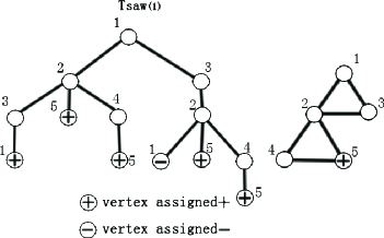
Figure 1: The graph with one vertex assigned + (Right) and its corresponding self-avoiding tree $T_{saw(1)}$ (Left)

A self-avoiding walk (SAW) is a sequence of moves (on a graph) which does not visit the same point more than once. The following gives an important tool in proving our results. It is introduced in[15].

Definition 2. (Self-Avoiding Tree) The self-avoiding tree $T_{saw(v)}(G)$ (for simplicity denoted by $T_{saw(v)}$) corresponding to the vertex $v$ of $G$ is the tree with root $v$ and generated through the self-avoiding walks originating at $v$. A vertex closing a cycle is included as a leaf of the tree and is assigned to be $+$, if the edge ending the cycle is larger than the edge starting the cycle, and $-$ otherwise.

Remark: Given any configuration $\sigma_{\Lambda}$ of $G$, $\Lambda\subset V$, the self-avoiding tree is constructed in the same way as the above procedure except that the vertex, which is a copy of the vertex $i$ in $\Lambda$, is fixed to the same spin $\sigma_{i}$ as $i$ and the subtree below it is not constructed due to the Markov property, see Figure 1 for example, where vertex $5$ is fixed $+$ in $G$.

Definition 3. (Strong Correlation Decay) The Gibbs distribution of two-state spin systems on $G$ exhibits strong correlation decay if and only if for any vertex $v\in V$, subset $\Lambda\subset V$, any two configurations $\sigma_{\Lambda}$ and $\eta_{\Lambda}$ on $\Lambda$, denote $t=d(v,\Theta)$, where $\Theta=\{v\in\Lambda:\sigma_{v}\neq\eta_{v}\}$, there exits positive numbers $a$, $b$ independent of $n$ such that

$$|\log P_{G}(X_{v}=+|\sigma_{\Lambda})-\log P_{G}(X_{v}=+|\eta_{\Lambda})|\leq f(t),$$

where decay function $f(t)=a\exp(-bt)$.

Definition 4. (FPTAS) An approximation algorithm is called a fully polynomial time approximation scheme (FPTAS) if and only if for any $\epsilon>0$, it takes a polynomial time of input and $\epsilon^{-1}$ to output a value $\bar{M}$ satisfying

$$e^{-\epsilon}\leq\frac{\bar{M}}{M}\leq e^{\epsilon},$$

where $M$ is the real value.

3. Strong Correlation Decay

In two-state spin systems, when $\beta_{ij}(\sigma_{i},\sigma_{j})=J_{ij}\sigma_{i}\sigma_{j}$, $h_{i}=B_{i}\sigma_{i}$ for all the edge $(i,j)\in E$ and vertex $i\in V$, and $J_{ij}$ is uniformly negative$/$positive for all $(i,j)\in E$, the system is called antiferromagnetic/ferromagnetic Ising model. Let

$$J_{ij}=\frac{\beta_{ij}(+,+)+\beta_{ij}(-,-)-\beta_{ij}(-,+)-\beta_{ij}(+,-)}{4},$$

and $B_{i}=\frac{h_{i}(+)-h_{i}(-)}{2}$ for all edges and vertices. We call $J_{ij}$ and $B_{i}$ ‘inverse temperature’ and ‘external field’ of two-state spin systems. Let $J=\max_{(i,j)\in E}|J_{ij}|$. The main theorem in this section is summarized as follows

Theorem 1. Let $G=(V,E)$ be a graph with vertex set $V=\{1,2,\cdots,n\}$ and edge set $E$. There exists a numbers $d>0$ such that $\Delta(G)\leq d$. Suppose

$$(d-1)\tanh{J}<1,$$

that is equivalent to $J<J_{d}=\frac{1}{2}\log(\frac{d}{d-2})$, then the Gibbs distribution of the two-state spin systems on $G$ exhibits strong correlation decay for arbitrary external field. Specifically, decay function is

$$f(t)=4Jd((d-1)\tanh J)^{t-1}.$$

In order to prove Theorem 1, four technical lemmas are given first. The inequality in Lemma 1 is inspired by a similar result in [10].

Lemma 1. Let $a$, $b$, $c$, $d$, $x$, $y$ be positive numbers, $g(x)=\frac{ax+b}{cx+d}$ and $t=|\frac{\sqrt{ad}-\sqrt{bc}}{\sqrt{ad}+\sqrt{bc}}|$, then

$$\max(\frac{g(x)}{g(y)},\frac{g(y)}{g(x)})\leq(\max(\frac{x}{y},\frac{y}{x}))^{t}.$$

Proof. We separate the proof into two cases.

Case 1. $ad\geq bc$. Consider a function

$$g(x)=\frac{ax+b}{cx+d}=\frac{a}{c}-\frac{ad-bc}{c(cx+d)}.$$

It is clearly an increasing function. Without loss of the generality, suppose $x\geq y$ and let $x=zy$, where $z\geq 1$, then

$$\begin{split}\log(\frac{g(x)}{g(y)})&=\int^{z}_{1}\frac{d(\log(\frac{g(\alpha y)}{g(y)}))}{d\alpha}d\alpha=\int^{z}_{1}(\frac{ay}{a\alpha y+b}-\frac{cy}{c\alpha y+d})d\alpha\\ &=\int^{z}_{1}\frac{(ad-bc)y}{(a\alpha y+b)(c\alpha y+d)}d\alpha\\ &=\int^{z}_{1}\frac{(ad-bc)y}{(\sqrt{ac}\alpha y-\sqrt{bd})^{2}+(\sqrt{bc}+\sqrt{ad})^{2}\alpha y}d\alpha\\ &\leq\int^{z}_{1}\frac{(ad-bc)y}{(\sqrt{bc}+\sqrt{ad})^{2}\alpha y}d\alpha=\frac{\sqrt{ad}-\sqrt{bc}}{\sqrt{ad}+\sqrt{bc}}\log z.\end{split}$$

Hence

$$\max(\frac{g(x)}{g(y)},\frac{g(y)}{g(x)})=\frac{g(x)}{g(y)}\leq(\frac{x}{y})^{t}=(\max(\frac{x}{y},\frac{y}{x}))^{t},$$

where $t=\frac{\sqrt{ad}-\sqrt{bc}}{\sqrt{ad}+\sqrt{bc}}$.
Case 2. $ad\leq bc$. Now $g(x)$ is a decreasing function. Let $h(x)=1/g(x)$, then $h(x)$ is an increasing function. Suppose $x\geq y$, it is easy to be obtained that

$$\frac{h(x)}{h(y)}\leq(\frac{x}{y})^{\frac{\sqrt{bc}-\sqrt{ad}}{\sqrt{ad}+\sqrt{bc}}}.$$

Hence

$$\max(\frac{g(x)}{g(y)},\frac{g(y)}{g(x)})=\frac{g(y)}{g(x)}=\frac{h(x)}{h(y)}\leq(\frac{x}{y})^{t}=(\max(\frac{x}{y},\frac{y}{x}))^{t},$$

where $t=\frac{\sqrt{bc}-\sqrt{ad}}{\sqrt{ad}+\sqrt{bc}}$.    $\Box$

Lemma 2. Let $T=T(V,E)$ be a rooted tree with vertex set $V=\{0,1,2,\cdots,n\}$ and edge set $E$. The root is vertex $0$. Suppose some vertices are fixed(assigned to certain spins) on $T$. Removing an edge $(k,l)$, where $d(k,0)<d(l,0)$, let $T_{k}$ and $T_{l}$ be two resulting subtrees of $T$ including vertex $k$ and $l$ respectively. The fixed vertices remain fixed on $T_{k}$ and $T_{l}$. Then the probability $P(X_{0}=+\ on\ T)$ equals the probability $P(X_{0}=+\ on\ the\ subtree\ T_{k})$ except changing the ‘external field’ $h_{k}$ to certain value $h^{{}^{\prime}}_{k}$ on $T_{k}$.

Proof. Let $\Omega_{T_{l}}$ denote the configuration space on $T_{l}$. $E_{l}$ and $V_{l}$ denote the edge set and vertex set on $T_{l}$. The following equality implies the result of the lemma.

$$\begin{split}h^{{}^{\prime}}_{k}(\sigma_{k})&=h_{k}(\sigma_{k})+\log(\sum\limits_{\tau\in\Omega_{T_{l}}}e^{\beta_{kl}(\sigma_{k},\tau_{l})+\sum\limits_{(i,j)\in E_{l}}\beta_{ij}(\tau_{i},\tau_{j})+\sum\limits_{i\in V_{l}}h_{i}(\tau_{i})}).\ \ \ \ \ \ \ \Box\end{split}$$

With Lemma 1 and Lemma 2, strong correlation decay property on trees will be proved.

Lemma 3. Let $T=T(V,E)$ be a rooted tree with vertex set $V=\{0,1,2,\cdots,n\}$ and edge set $E$. The root is vertex $0$. Consider the two-state spin systems on it. Let $\Lambda\subset V$ , $\zeta_{\Lambda}$ and $\eta_{\Lambda}$ be any two configurations on $\Lambda$. Let $\Theta=\{i:\zeta_{i}\neq\eta_{i},i\in\Lambda\}$, $t=d(0,\Theta)$ and $s=|S(T,0,t)|=|\{i:d(0,i)=t,i\in T\}|$. Then

$$\begin{split}\max(\frac{P_{T}(X_{0}=+|\zeta_{\Lambda})}{P_{T}(X_{0}=+|\eta_{\Lambda})},\frac{P_{T}(X_{0}=+|\eta_{\Lambda})}{P_{T}(X_{0}=+|\zeta_{\Lambda})})\leq e^{4Js(\tanh{J})^{t-1}}.\end{split}$$

Proof. For any $i\in V$, let $T_{i}$ denote the subtree with $i$ as its root and $Z(i)$ be the two-state spin systems induced on $T_{i}$ by $T$. Note that $T_{0}$ is equal to $T$. To prove the theorem, it’s convenient to deal with the ratio $\frac{P_{T}(X_{0}=+|\zeta_{\Lambda})}{P_{T}(X_{0}=-|\zeta_{\Lambda})}$ rather than $P_{T}(X_{0}=+|\zeta_{\Lambda})$ itself. Denote $R^{\zeta_{\Lambda}}_{i}\equiv\frac{P_{T_{i}}(X_{i}=+|\zeta_{\Lambda_{i}})}{P_{T_{i}}(X_{i}=-|\zeta_{\Lambda_{i}})}$, where $\zeta_{\Lambda_{i}}$ is the condition by imposing the configuration $\zeta_{\Lambda}$ on $T_{i}$. When $x_{1},x_{2}\in(0,1)$, $\frac{x_{1}}{x_{2}}\geq 1$ if and only if $\frac{x_{1}}{1-x_{1}}\geq\frac{x_{2}}{1-x_{2}}$. Then

$$\max\{\frac{x_{1}}{x_{2}},\frac{x_{2}}{x_{1}}\}\leq\max\{\frac{x_{1}/(1-x_{1})}{x_{2}/(1-x_{2})},\frac{x_{2}/(1-x_{2})}{x_{1}/(1-x_{1})}\}.$$

Replace $x_{1}$ and $x_{2}$ by $P_{T}(X_{0}=+|\zeta_{\Lambda})$ and $P_{T}(X_{0}=+|\eta_{\Lambda})$. Then lemma 2 follows by

$$\max(\frac{P_{T}(X_{0}=+|\zeta_{\Lambda})}{P_{T}(X_{0}=+|\eta_{\Lambda})},\frac{P_{T}(X_{0}=+|\eta_{\Lambda})}{P_{T}(X_{0}=+|\zeta_{\Lambda})})\leq\max(\frac{R^{\zeta_{\Lambda}}_{0}}{R^{\eta_{\Lambda}}_{0}},\frac{R^{\eta_{\Lambda}}_{0}}{R^{\zeta_{\Lambda}}_{0}}).$$

Hence what is needed to be proved becomes

$$\max(\frac{R^{\zeta_{\Lambda}}_{0}}{R^{\eta_{\Lambda}}_{0}},\frac{R^{\eta_{\Lambda}}_{0}}{R^{\zeta_{\Lambda}}_{0}})\leq\exp(4Js(\tanh{J})^{t-1}).$$ (1)

The inequality (1) is proved by induction on $t$. Before doing it, some trivial cases need to be clarified. We are interested in the case $t\geq 1$ and $0$ is unfixed. Let $\Gamma_{kl}$ denote the unique self-avoiding path from $k$ to $l$ on $T$. If $i$ is a leaf on $T$ and $d(0,i)<t$, where $t=d(0,\Theta)$, define $U_{i}=\{j\in V:j\in\Gamma_{0i},\exists k\in S(T,0,t),s.t.j\in\Gamma_{0k}\}$. $U_{i}\neq\emptyset$ because of $0\in U_{i}$. Let $j_{i}\in U_{i}$ such that $d(i,j_{i})=d(i,U_{i})$. By lemma 2, we can remove the subtree bellow $j_{i}$ and change external field from $h_{j_{i}}$ to $h^{{}^{\prime}}_{j_{i}}$ at $j_{i}$ without changing the probability $P(X_{0}=+)$. It is noted that this procedure removes at least one leaf with the hight $<t$, and does not remove any vertex with the hight $\geq t$. We can suppose that $T$ is a tree rooted at $0$ and the height of every leaf on the tree is no less than $t$. Let $0_{1},0_{2},\cdots,0_{q}$ be the neighbors connecting with $0$. The recursive formula can be presented. Let $\Omega_{T_{i}}$ denote the configuration space in $T_{i}$ under the condition $\zeta_{\Lambda}$, $i=1,2,\cdots,q$ and $\Omega_{0}$ denote the configuration space of $T_{0}$ under the condition $\zeta_{\Lambda}\cup\{\sigma_{0}\}$. We have

$$\begin{split}&R^{\zeta_{\Lambda}}_{0}=\frac{Z(T_{0},X_{0}=+,\zeta_{\Lambda})}{Z(T_{0},X_{0}=-,\zeta_{\Lambda})}\\ &=\frac{e^{h_{0}(+)}\sum\limits_{\sigma\in\Omega_{0}}e^{\sum\limits_{i=1}^{q}(\beta_{00_{i}}(+,\sigma_{0_{i}})+\sum\limits_{(k,l)\in T_{i}}\beta_{kl}(\sigma_{k},\sigma_{l})+\sum\limits_{k\in T_{i}}h_{k}(\sigma_{k}))}}{e^{h_{0}(-)}\sum\limits_{\sigma\in\Omega_{0}}e^{\sum\limits_{i=1}^{q}(\beta_{00_{i}}(-,\sigma_{0_{i}})+\sum\limits_{(k,l)\in T_{i}}\beta_{kl}(\sigma_{k},\sigma_{l})+\sum\limits_{k\in T_{i}}h_{k}(\sigma_{k}))}}\\ &=e^{2B_{0}}\prod\limits^{q}_{i=1}\frac{\sum\limits_{\sigma\in\Omega_{T_{i}}}e^{\beta_{00_{i}}(+,\sigma_{0_{i}})+\sum\limits_{(k,l)\in T_{i}}\beta_{kl}(\sigma_{k},\sigma_{l})+\sum\limits_{k\in T_{i}}h_{k}(\sigma_{k})}}{\sum\limits_{\sigma\in\Omega_{T_{i}}}e^{\beta_{00_{i}}(-,\sigma_{0_{i}})+\sum\limits_{(k,l)\in T_{i}}\beta_{kl}(\sigma_{k},\sigma_{l})+\sum\limits_{k\in T_{i}}h_{k}(\sigma_{k})}}\\ \end{split}$$

$$\begin{split}&=e^{2B_{0}}\prod\limits^{q}_{i=1}\frac{a_{i}Z(T_{0_{i}},X_{i}=+,\zeta_{\Lambda_{i}})+b_{i}Z(T_{0_{i}},X_{i}=-,\zeta_{\Lambda_{i}})}{c_{i}Z(T_{0_{i}},X_{i}=+,\zeta_{\Lambda_{i}})+d_{i}Z(T_{0_{i}},X_{i}=-,\zeta_{\Lambda_{i}})}\\ &=e^{2B_{0}}\prod\limits^{q}_{i=1}\frac{a_{i}R^{\zeta_{\Lambda}}_{0_{i}}+b_{i}}{c_{i}R^{\zeta_{\Lambda}}_{0_{i}}+d_{i}},\end{split}$$ (2)

where $B_{0}=\frac{h_{0}(+)-h_{0}(-)}{2}$, $a_{i}=e^{\beta_{00_{i}}(+,+)}$, $b_{i}=e^{\beta_{00_{i}}(+,-)}$, $c_{i}=e^{\beta_{00_{i}}(-,+)}$, $d_{i}=e^{\beta_{00_{i}}(-,-)}$ . Now checking the base case $t=1$ where $R^{\zeta_{\Lambda}}_{0_{i}},R^{\eta_{\Lambda}}_{0_{i}}\in[0,+\infty]$, by the monotonicity of $\frac{a_{i}R^{\zeta_{\Lambda}}_{0_{i}}+b_{i}}{c_{i}R^{\zeta_{\Lambda}}_{0_{i}}+d_{i}}$ and $\frac{a_{i}R^{\eta_{\Lambda}}_{0_{i}}+b_{i}}{c_{i}R^{\eta_{\Lambda}}_{0_{i}}+d_{i}}$,

$$\begin{split}\max(\frac{R^{\zeta_{\Lambda}}_{0}}{R^{\eta_{\Lambda}}_{0}},\frac{R^{\eta_{\Lambda}}_{0}}{R^{\zeta_{\Lambda}}_{0}})&\leq\prod\limits^{q}_{i=1}\max(\frac{a_{i}d_{i}}{b_{i}c_{i}},\frac{b_{i}c_{i}}{a_{i}d_{i}})\leq e^{4qJ}.\end{split}$$

Hence, (1) holds when $t=1$. By induction, assume that (1) holds for $t-1$, we will show that it holds for $t$. Let $s_{i}=|S(T_{0_{i}},0_{i},t-1)|$, $i=1,2,\cdots,q$, repeating above recursive procedure, then

$$\begin{split}\max(\frac{R^{\zeta_{\Lambda}}_{0}}{R^{\eta_{\Lambda}}_{0}},\frac{R^{\eta_{\Lambda}}_{0}}{R^{\zeta_{\Lambda}}_{0}})&\leq\prod\limits^{q}_{i=1}\max(\frac{\frac{a_{i}R^{\zeta_{\Lambda}}_{0_{i}}+b_{i}}{c_{i}R^{\zeta_{\Lambda}}_{0_{i}}+d_{i}}}{\frac{a_{i}R^{\eta_{\Lambda}}_{0_{i}}+b_{i}}{c_{i}R^{\eta_{\Lambda}}_{0_{i}}+d_{i}}},\frac{\frac{a_{i}R^{\eta_{\Lambda}}_{0_{i}}+b_{i}}{c_{i}R^{\eta_{\Lambda}}_{0_{i}}+d_{i}}}{\frac{a_{i}R^{\zeta_{\Lambda}}_{0_{i}}+b_{i}}{c_{i}R^{\zeta_{\Lambda}}_{0_{i}}+d_{i}}})\\ &\leq\prod\limits^{q}_{i=1}\max(\frac{R^{\zeta_{\Lambda}}_{0_{i}}}{R^{\eta_{\Lambda}}_{0_{i}}},\frac{R^{\eta_{\Lambda}}_{0_{i}}}{R^{\zeta_{\Lambda}}_{0_{i}}})^{|\frac{\sqrt{a_{i}d_{i}}-\sqrt{b_{i}c_{i}}}{\sqrt{a_{i}d_{i}}+\sqrt{b_{i}c_{i}}}|}\\ &\leq\prod\limits^{q}_{i=1}\max(\frac{R^{\zeta_{\Lambda}}_{0_{i}}}{R^{\eta_{\Lambda}}_{0_{i}}},\frac{R^{\eta_{\Lambda}}_{0_{i}}}{R^{\zeta_{\Lambda}}_{0_{i}}})^{\tanh J},\end{split}$$

where the second inequality comes from Lemma 1. According to the hypothesis of induction $\max(\frac{R^{\zeta_{\Lambda}}_{0_{i}}}{R^{\eta_{\Lambda}}_{0_{i}}},\frac{R^{\eta_{\Lambda}}_{0_{i}}}{R^{\zeta_{\Lambda}}_{0_{i}}})\leq\exp(4Js_{i}(\tanh{J})^{t-2})$, it’s sufficient to show

$$\begin{split}\max(\frac{R^{\zeta_{\Lambda}}_{0}}{R^{\eta_{\Lambda}}_{0}},\frac{R^{\eta_{\Lambda}}_{0}}{R^{\zeta_{\Lambda}}_{0}})&\leq\prod\limits^{q}_{i=1}\exp(4Js_{i}(\tanh{J})^{t-1})\\ &=\exp(4Js(\tanh{J})^{t-1}),\end{split}$$

where the last equation follows by $\sum_{i=1}^{q}s_{i}=s$. This completes the proof.    $\Box$

To generalize the strong correlation decay property on trees to the general graphs, we need to utilize the remarkable property of the self-avoiding tree, which is implicitly stated in [15] and explicitly stated in [8].
Lemma 4 ([8]). For two-state spin systems on $G=(V,E)$, for any configuration $\sigma_{\Lambda}$, $\Lambda\subset V$ and any vertex $v\in V$, then

$$P_{G}(X_{v}=+|\sigma_{\Lambda})=P_{T_{saw(v)}}(X_{v}=+|\sigma_{\Lambda}).$$

With Lemma 3 and 4, it is enough to prove Theorem 1.

Proof of Theorem 1. Since the maximum degree of $T_{saw(i)}$ is also bounded by $d$, obviously, $s=|S(T_{saw(i)},i,t)|\leq d(d-1)^{t-1}$. According to Lemma 3 and 4, Theorem 1 is proved.     $\Box$

Remark: From the proof of Theorem 1, by a similar argument, we can get

$$|\log P_{G}(X_{v}=-|\sigma_{\Lambda})-\log P_{G}(X_{v}=-|\eta_{\Lambda})|\leq f(t),$$

where $f(t)=4Jd((d-1)\tanh J)^{t-1}$.

As one of the corollaries of strong correlation decay property, we prove there is unique Gibbs measure on an infinite bounded degree graph (an infinite graph with maximum degree over all the degree of its vertices $\leq d$). This generalizes original Dobrushion’s condition

$$d\tanh J<1\ to\ (d-1)\tanh J<1$$

for uniqueness of Gibbs measure of Ising models[4].

Theorem 2. Let $\mathbf{G}$ be an infinite graph and $\Delta(\mathbf{G})=\sup\limits_{i\in\mathbf{G}}\{\delta_{i}\}$. Assume there exists a constant $d$ such that $\Delta(\mathbf{G})\leq d$. There is a two-state spin systems on each sub finite graph $G$ of $\mathbf{G}$ which is defined by Definition 1. If $(d-1)\tanh J<1$, then the Gibbs measure on $\mathbf{G}$ corresponding to the two-state spin systems on sub finite graphs is unique.

Proof. For any given finite sub graph $G=(V,E)$ of $\mathbf{G}$, let $\partial G=\{i:(i,j)\in\mathbf{G},i\notin G,j\in G\}$ and $G=G_{0}$. Suppose there is a sequence of finite sub graphs $G_{n-1}\subset G_{n}$ of $\mathbf{G}$, $n=1,2,\cdots,\infty$ such that $d_{n}=d(G,\partial G_{n})$ goes to infinity as $n\rightarrow\infty$. Let $G^{\prime}_{n}=G_{n}\cup\partial G_{n}$ and denote $\zeta_{n}$, $\eta_{n}$ any two configurations on $\partial G_{n}$, for $n=1,2,\cdots,\infty$. Let $\sigma_{\Lambda}$ be any configuration on $\Lambda$, $\Lambda\subset V$. By Proposition 2.2 in [14], the Gibbs measure is unique on $\mathbf{G}$ if

$$\lim\limits_{n\rightarrow\infty}\sup\limits_{\zeta_{n},\eta_{n}}\max\limits_{\Lambda\subset V,\sigma_{\Lambda}}|P_{G^{\prime}_{n}}(X_{\Lambda}=\sigma_{\Lambda}|\zeta_{n})-P_{G^{\prime}_{n}}(X_{\Lambda}=\sigma_{\Lambda}|\eta_{n})|=0$$

holds. Let $\Lambda=\{1,2,\cdots,m\}$, where $m=|\Lambda|$. Set $\alpha_{n}(1)=P_{G^{\prime}_{n}}(X_{1}=\sigma_{1}|\zeta_{n})$ and $\beta_{n}(1)=P_{G^{\prime}_{n}}(X_{1}=\sigma_{1}|\eta_{n})$. Let $\alpha_{n}(i)=P_{G^{\prime}_{n}}(X_{i}=\sigma_{i}|\zeta_{n},\sigma_{j},1\leq j\leq i-1)$ and $\beta_{n}(i)=P_{G^{\prime}_{n}}(X_{i}=\sigma_{i}|\eta_{n},\sigma_{j},1\leq j\leq i-1)$, $i=2,3,\cdots,n$. The telescoping trick gives

$$P_{G^{\prime}_{n}}(X_{\Lambda}=\sigma_{\Lambda}|\zeta_{n})=\prod\limits^{m}_{i=1}\alpha_{n}(i)$$

and $P_{G^{\prime}_{n}}(X_{\Lambda}=\sigma_{\Lambda}|\eta_{n})=\prod\limits^{m}_{i=1}\beta_{n}(i)$. By Theorem 1 and above remark, we know, for each $i\in\Lambda$,

$$|\log(\frac{\alpha(i)}{\beta(i)})|\leq f(d_{n}),$$

where $f(t)$ is the decay function $f(t)=4Jd((d-1)\tanh J)^{t-1}$. Then

$$\log(\prod\limits^{m}_{i=1}\frac{\alpha(i)}{\beta(i)})\leq mf(d_{n}),$$

where $m=|\Lambda|$. Hence

$$\sup\limits_{\zeta_{n},\eta_{n}}\max\limits_{\Lambda\subset V,\sigma_{\Lambda}}\log(\frac{P_{G^{\prime}_{n}}(X_{\Lambda}=\sigma_{\Lambda}|\zeta_{n})}{P_{G^{\prime}_{n}}(X_{\Lambda}=\sigma_{\Lambda}|\eta_{n})})\leq|V|f(d_{n}).$$

Therefore, if $(d-1)\tanh J<1$, then

$$\lim_{n\rightarrow\infty}\sup\limits_{\zeta_{n},\eta_{n}}\max\limits_{\Lambda\subset V,\sigma_{\Lambda}}\log(\frac{P_{G^{\prime}_{n}}(X_{\Lambda}=\sigma_{\Lambda}|\zeta_{n})}{P_{G^{\prime}_{n}}(X_{\Lambda}=\sigma_{\Lambda}|\eta_{n})})=0.\$$

This completes the proof.    $\Box$

4. Approximating the Partition Function

In the proof of Lemma 3, the calculation of the marginal probability of the root yields a local recursive procedure. If the tree is truncated at height $t$, and using the recursive formula (2) to compute the marginal probability at the root, it is easy to see that the complexity of this procedure is linear with the number of vertices of the truncated tree. Let $\Phi_{1}$ denote the whole state space, which means $P_{G}(X_{1}=+|\Phi_{1})=P_{G}(X_{1}=+)$, and $\Phi_{j}=\{X_{i}=+,1\leq i\leq j-1\}$, $2\leq j\leq n+1$. Let $\widehat{p_{j}}$ an estimator of conditional marginal probability $p_{j}=P_{G}(X_{j}=+|\Phi_{j})$, $j=1,2,\cdots,n$. The algorithm to compute the partition function is proposed as follows.

Algorithm for Partition Function $Z(G$)
Input: $G$, a graph with vertices $\{1,\cdots,n\}$, the two-state spin systems on $G$, $\epsilon>0$, precision;
Output: $\widehat{Z(G)}$, the estimator of partition function $Z(G)$.
begin

For $j$ from $1$ to $n$ do

step 1. Set $t_{j}=\frac{\log(4nJd\epsilon^{-1})}{\log((d-1)tanhJ)^{-1}}+1$,

step 2. Take the vertex $j$ as root and generate the truncated subtree $T^{\prime}_{saw(j)}$ with height $t_{j}$

under the condition $\Phi_{j}$,

step 3. Set initial values be $0^{\prime}s$ for all the vertices of $T^{\prime}_{saw(j)}$ at height $t_{j}$ ,

step 4. Computing $\widehat{p_{j}}$ through $T^{\prime}_{saw(j)}$ by recursive formula (2).

End For

Compute $\widehat{Z(G)}=Z(G,\Phi_{n+1})\prod\limits^{n}_{i=1}\widehat{p_{i}}^{-1}$.
end

Theorem 3. Let $G=(V,E)$ be a graph with vertex set $V=\{1,2,\cdots,n\}$ and edge set $E$. There exists a positive number $d>0$ such that $\Delta(G)\leq d$. If $J<J_{d}$, then the above algorithm provides an FPTAS for partition function of the two-state spin systems on $G$.

Proof. According to the results of Theorem 1, there is a function $f(t_{j})\leq\frac{\epsilon}{n}$, such that

$$e^{-\frac{\epsilon}{n}}\leq\frac{p_{j}}{\widehat{p_{j}}}\leq e^{\frac{\epsilon}{n}},$$

under the condition that

$$t_{j}=\frac{\log(4nJd\epsilon^{-1})}{\log((d-1)tanhJ)^{-1}}+1=O(\log n+\log(\epsilon^{-1})).$$

Since $p_{j}=\frac{Z(G,\Phi_{j+1})}{Z(G,\Phi_{j})}$, $Z(G)$ can be expressed as the product $Z(G)=Z(G,\Phi_{n+1})\prod\limits^{n}_{i=1}p_{i}^{-1}$. Hence,

$$e^{-\epsilon}\leq e^{(-\frac{\epsilon}{n})n}\leq\prod\limits^{n}_{i=1}\frac{\widehat{p_{i}}^{-1}}{p_{i}^{-1}}=\frac{\widehat{Z(G)}}{Z(G)}\leq e^{(\frac{\epsilon}{n})n}\leq e^{\epsilon}.$$

The complexity of the algorithm for each $j$ in the loop is

$$O(|V(T_{saw(j)},j,t_{j})|)=O((d-1)^{t_{j}}).$$

Thus, the total complexity of the algorithm is

$$\sum\limits_{j}O((d-1)^{O(\log n+\log(\epsilon^{-1}))})=nO((d-1)^{O(\log n+\log(\epsilon^{-1}))})=O(n^{O(1)}+n(\epsilon^{-1})^{O(1)}),$$

which completes the proof.     $\Box$

5. Conclusions and Discussions

We show that the Gibbs distribution of two-state spin systems on a bounded degree graph $G=(V,E)$ with maximum degree $d$ exhibits strong correlation decay when $J<J_{d}$. By the strong correlation decay property and the self-avoiding tree technique, we prove the uniqueness of Gibbs measure on an infinite bounded degree graph, which generalizes original Dobrushion’s condition $d\tanh(J)<1$ to $(d-1)\tanh(J)<1$ for uniqueness of Gibbs measure of (anti)ferromagnetic Ising models. Since $J_{d}$ is the critical point for uniqueness of Gibbs measure on an infinite $d$ regular tree of Ising model. This implies that the condition for inverse temperature is tight when restricting it on Ising model.

It is not difficult to apply our results to the sparse on average graphs [11] and Erd$\ddot{o}$s-R$\dot{e}$nyi random graph $G(n,d/n)$, where each edge is chosen independently with probability $d/n$ [11]. We also present an FPTAS for partition functions of two-state spin systems on the bounded degree graphs. An interesting investigation could be whether the condition is sharp for the general two-state spin systems.

References

• [1] A. Bandyopadhyay and D. Gamarnik, Counting without sampling: New algorithms for enumeration problems using statistical physics, Proceedings of 17th ACM-SIAM Symposium on Discrete Algorithms (SODA) (2006), 890-899.
• [2] A. Dembo and A. Montanari, Ising models on locally tree-like graphs, Preprint on http://arXiv:0804.4726v2
• [3] R.L. Dobrushin, Prescibing a system of random variables by the help of conditional distributions, Theory Probability and its Application 15(1970), 469-497.
• [4] H. O. Georgii, Gibbs measures and phase transitions, volume 9 of de Gruyter Studies in Mathematics. Walter de Gruyter $\&$ Co., Berlin, (1988).
• [5] L. A. Goldberg, M.Jerrum and M. Paterson, The Computational Complexity of Two-State Spin Systems, Random Structures and Algorithms 23 (2003), 133-154.
• [6] M. Jerrum and A. Sinclair, Polynomial-time approximation algorithms for Ising model, SIAM J. Comput. Vol22, No. 5, (1993), 1087-1116.
• [7] J. Jonasson, Uniqueness of uniform random colorings of regular trees, Statistics and Probability Letters 57 (2002), 243-248.
• [8] K. Jung and D. Shah, Inference in Binary Pair-wise Markov Random Field through Self-Avoiding Walk, Preprint on http://arxiv.org/abs/cs.AI/0610111v2.
• [9] M. Jerrum, L. Valiant, and V. Vazirani, Random generation of combinatorial structures from a uniform distribution, Theoret. Comput. Sci. 43. (1986), 169-188.
• [10] R. Lyons, The Ising model and percolation on trees and treelike graphs, Comm. Math. Phys., 125(2), (1989), 337-353.
• [11] E. Mossel and A. Sly, Rapid mixing of gibbs sampling on graphs that are sparse on average, Proceedings of 19th ACM-SIAM Symposium on Discrete Algorithms (SODA), (2008), 238-247.
• [12] R. Pemantle and Y. Peres, The critical Ising model on trees, concave recursions and nonlinear capacity, http://arxiv.org/PS_cache/math/pdf/0503/0503137v2.
• [13] L. G. Valiant, The complexity of computing the permanent, Theoretical Computer Science 8 (1979), 189-201.
• [14] D. Weitz, combinatorial cirteria for uniqueness of Gibbs measures, Random Structures and Algorithms 27, (2005), 445-475.
• [15] D. Weitz, Counting indpendent sets up to the tree threshold, Proceedings of the 38th annual ACM symposium on Theory of computing(STOC), (2006), 140-149.