Sparse Empirical Bayes Analysis (SEBA)

Abstract

We consider a joint processing of $n$ independent sparse regression problems. Each is based on a sample $(y_{i1},x_{i1})\dots,(y_{im},x_{im})$ of $m$ i.i.d. observations from $y_{i1}=x_{i1}^{\scriptstyle{\mathsf{T}}}\beta_{i}+\varepsilon_{i1}$, $y_{i1}\in{\mathbb{R}}$, $x_{i1}\in{\mathbb{R}}^{p}$, $i=1,\dots,n$, and $\varepsilon_{i1}\sim N(0,\sigma^{2})$, say. $p$ is large enough so that the empirical risk minimizer is not consistent. We consider three possible extensions of the lasso estimator to deal with this problem, the lassoes, the group lasso and the RING lasso, each utilizing a different assumption how these problems are related. For each estimator we give a Bayesian interpretation, and we present both persistency analysis and non-asymptotic error bounds based on restricted eigenvalue - type assumptions.

“…and only a star or two set sparsedly in the vault of heaven; and you will find a sight as stimulating as the hoariest summit of the Alps.” R. L. Stevenson

1 Introduction

We consider the model

$$\begin{split}\allowdisplaybreaks Y_{i}=X_{i}^{\scriptstyle{\mathsf{T}}}\beta_{i}+\varepsilon_{i},\quad i=1,\dots,n,\end{split}$$ (1)

or more explicitly

$$y_{ij}=x_{ij}^{\scriptstyle{\mathsf{T}}}\beta_{i}+\varepsilon_{ij},\quad i=1,\dots,n,\;j=1,\dots,m$$

where $\beta_{i}\in{\mathbb{R}}^{p}$, $X_{i}\in{\mathbb{R}}^{m\times p}$ is either deterministic fixed design matrix, or a sample of $m$ independent ${\mathbb{R}}^{p}$ random vectors. Generally, we think of $j$ indexing replicates (of similar items within the group) and $i$ indexing groups (of replicates). Finally, $\varepsilon_{ij}$, $i=1,\dots,n,\;j=1,\dots,m$ are (at least uncorrelated with the $x$s), but typically assumed to be i.i.d. sub-Gaussian random variables, independent of the regressors $x_{ij}$. We can consider this as $n$ partially related regression models, with $m$ i.i.d. observations on the each model. For simplicity, we assume that all variables have expectation 0. The fact that the number of observations does not dependent on $i$ is arbitrary and is assumed only for the sake of notational simplicity.

The standard FDA (functional data analysis) is of this form, when the functions are approximated by their projections on some basis. Here we have $n$ i.i.d. random functions, and each group can be considered as $m$ noisy observations, each one is on the value of these functions at a given value of the argument. Thus,

$$\begin{split}\allowdisplaybreaks y_{ij}=g_{i}(z_{ij})+\varepsilon_{ij},\end{split}$$ (2)

where $z_{ij}\in[0,1]$. The model fits the regression setup of 1, if $g(z)=\sum_{\ell=1}^{p}\beta_{\ell}h_{\ell}(p)$ where $h_{1},\dots,h_{p}$ are in $L_{2}(0,1)$, and $x_{ij\ell}=h_{\ell}(z_{ij})$.

This approach is in the spirit of the empirical Bayes approach (or compound decision theory, note however that the term “empirical Bayes” has a few other meanings in the literature), cf, [11, 12, 8]. The empirical Bayes to sparsity was considered before, e.g., [15, 3, 7, 6]. However, in these discussions the compound decision problem was within a single vector, while we consider the compound decision to be between the vectors, where the vectors are the basic units. The beauty of the concept of compound decision, is that we do not have to assume that in reality the units are related. They are considered as related only because our loss function is additive.

One of the standard tools for finding sparse solutions in a large $p$ small $m$ situation is the lasso (Tibshirani [13]), and the methods we consider are its extensions.

We will make use of the following notation. Introduce $l_{p,q}$ norm of a set of vectors $z_{1},\dots,z_{n}$, not necessarily of the same length, $z_{ij}$, $i=1,\dots,n$, $j=1,\dots,J_{i}$:

Definition 1.1

$||z||_{p,q}=\left[\sum_{i=1}^{n}\left(\sum_{j\in J_{i}}|z_{ij}|^{p}\right)^{q/p}\right]^{1/q}.$

These norms will serve as a penalty on the size of the matrix ${\mathcal{B}}=(\beta_{1},\dots,\beta_{n})$. Different norms imply different estimators, each appropriate under different assumptions.

Within the framework of the compound decision theory, we can have different scenarios, and we consider three of them. In Section 2 we investigate the situation when there is no direct relationship between the groups, and the only way the data are combined together is via the selection of the common penalty. In this case the sparsity pattern of the solution for each group are unrelated. We argue that the alternative formulation of the lasso procedure in terms of $\ell_{2,1}$ (or, more generally, $\ell_{\alpha,1}$) norm which we refer to as “lassoes” can be more natural than the simple lasso, and this is argued from different points of view.

The motivation is as follows. The lasso method can be described in two related ways. Consider the one group version, $y_{j}=x_{j}^{\scriptstyle{\mathsf{T}}}\beta+\varepsilon_{j}$. The lasso estimator can be defined by

$$\text{Minimize }\sum_{j=1}^{m}(y_{j}-x_{j}^{\scriptstyle{\mathsf{T}}}\beta)^{2}\quad\text{s.t.}\quad\|\beta\|_{1}<A.$$

An equivalent definition, using Lagrange multiplier is given by

$$\text{Minimize}\sum_{j=1}^{m}(y_{j}-x_{j}^{\scriptstyle{\mathsf{T}}}\beta)^{2}+\lambda\|\beta\|_{1}^{\alpha},$$

where $\alpha$ can be any arbitrarily chosen positive number. In the literature one can find almost only $\alpha=1$. One exception is Greenshtein and Ritov [5] where $\alpha=2$ was found more natural, also it was just a matter of aesthetics. We would argue that $\alpha>2$ may be more intuitive. Our first algorithm generalizes this representation of the lasso directly to deal with compound model 1.

In the framework of the compound decision problem it is possible to consider the $n$ groups as repeated similar models for $p$ variables, and to choose the variables that are useful for all models. We consider this in Section 3. The relevant variation of the lasso procedure in this case is group lasso introduced by Yuan and Lin [14]:

$$\begin{split}\allowdisplaybreaks\text{Minimize}\sum_{i=1}^{n}\sum_{j=1}^{m}(y_{ij}-x_{ij}^{\scriptstyle{\mathsf{T}}}\beta_{i})^{2}+\lambda\|\beta\|_{2,1}.\end{split}$$ (3)

The authors also showed that in this case the sparsity pattern of variables is the same (with probability 1). Non-asymptotic inequalities under restricted eigenvalue type condition for group lasso are given by Lounici et al. [10].

Now, the standard notion of sparsity, as captured by the $L_{0}$ norm, or by the standard lasso and group lasso, is basis dependent. Consider the model of 2. If, for example, $g(z)=\mbox{\Large$\mathbf{1}$}(a<z\leq b)$, then this example is sparse when $h_{\ell}(z)=\mbox{\Large$\mathbf{1}$}(z>\ell/p)$. It is not sparse if $h_{\ell}(z)=(z-\ell/p)^{+}$. On the other hand, a function $g$ which has a piece-wise constant slope is sparse in the latter basis, but not in the former, even though, each function can be represented equally well in both bases.

Suppose that there is a sparse representation in some unknown basis, but assumed common to the $n$ groups. The question arises, can we recover the basis corresponding to the sparsest representation? We will argue that this penalty, also known as trace norm or Schatten norm with $p=1$, aims in finding the rotation that gives the best sparse representation of all vectors instantaneously (Section 4). We refer to this method as the rotation-invariant lasso, or shortly as the RING lasso. This is not surprising as under some conditions, this penalty also solves the minimum rank problem (see Candes and Recht [4] for the noiselss case, and Bach [1] for some asymptotic results). By analogy with the lassoes argument, a higher power of the trace norm as a penalty may be more intuitive to a Bayesian.

For both procedures considered here, the lassoes and the RING lasso, we present the bounds on their persistency as well as non-asymptotic inequalities under restricted eigenvalues type condition. All the proofs are given in the Appendix.

2 The lassoes procedure

The minimal structural relationship we may assume is that the $\beta^{\prime}s$ are not related, except that we believe that there is a bound on the average sparsity of the $\beta$’s. One possible approach would be to consider the problem as a standard sparse regression problem with $nm$ observations, a single vector of coefficients $\beta=(\beta_{1}^{\scriptstyle{\mathsf{T}}},\dots,\beta_{n}^{\scriptstyle{\mathsf{T}}})^{\scriptstyle{\mathsf{T}}}$, and a block diagonal design matrix $X$. This solution imposes very little on the similarity among $\beta_{1},\dots,\beta_{n}$. The lassoes procedure discussed in this section assume that these vectors are similar, at least in their level of sparsity.

2.1 Prediction error minimization

In this paper we adopt an oracle point of view. Our estimator is the empirical minimizer of the risk penalized by the complexity of the solution (i.e., by its $\ell_{1}$ norm). We compare this estimator to the solution of an “oracle” who does the same, but optimizing over the true, unknown to simple human beings, population distribution.

We assume that each vector of $\beta_{i}$, $i=1,\dots,n$, solves a different problem, and these problems are related only through the joint loss function, which is the sum of the individual losses. To be clearer, we assume that for each $i=1,\dots,n$, $z_{ij}=(y_{ij},x_{ij}^{\scriptstyle{\mathsf{T}}})^{\scriptstyle{\mathsf{T}}}$, $j=1,\dots,m$ are i.i.d., sub-Gaussian random variables, drawn from a distribution $Q_{i}$. Let $z_{i}=(y_{i},x_{i}^{\scriptstyle{\mathsf{T}}})^{\scriptstyle{\mathsf{T}}}$ be an independent sample from $Q_{i}$. For any vector $a$, let $\tilde{a}=(-1,a^{\scriptstyle{\mathsf{T}}})^{\scriptstyle{\mathsf{T}}}$, and let $\tilde{}\Sigma_{i}$ be the covariance matrix of $z_{i}$ and $\mathfrak{S}=(\tilde{}\Sigma_{1},\dots,\tilde{}\Sigma_{n})$. The goal is to find the matrix $\hat{}{\mathcal{B}}=(\hat{}\beta_{1},\dots,\hat{}\beta_{n})$ that minimizes the mean prediction error:

$$\begin{split}\allowdisplaybreaks L({\mathcal{B}},\mathfrak{S})&=\sum_{i=1}^{n}{\rm E}\mathop{\!}\nolimits_{Q_{i}}(y_{i}-x_{i}^{\scriptstyle{\mathsf{T}}}\beta_{i})^{2}=\sum_{i=1}^{n}\tilde{}\beta_{i}^{\scriptstyle{\mathsf{T}}}\tilde{}\Sigma_{i}\tilde{}\beta_{i}.\end{split}$$ (4)

For $p$ small, the natural approach is empirical risk minimization, that is replacing $\tilde{}\Sigma_{i}$ in 4 by $\tilde{S}_{i}$, the empirical covariance matrix of $z_{i}$. However, generally speaking, if $p$ is large, empirical risk minimization results in overfitting the data. Greenshtein and Ritov [5] suggested (for the standard $n=1$) minimization over a restricted set of possible $\beta$’s, in particular, to either $L_{1}$ or $L_{0}$ balls. In fact, their argument is based on the following simple observations

$$\begin{split}\allowdisplaybreaks\bigl{|}\tilde{}\beta^{\scriptstyle{\mathsf{T}}}(\tilde{}\Sigma_{i}-\tilde{S}_{i})\tilde{}\beta\bigr{|}&\leq\|\tilde{}\Sigma_{i}-\tilde{S}_{i}\|_{\infty}\|\tilde{}\beta\|_{1}^{2}\\ &\text{and}\\ \|\tilde{}\Sigma_{i}-\tilde{S}_{i}\|_{\infty}&=\mathcal{O}_{p}(m^{-1/2}\log p)\end{split}$$ (5)

(see Lemma A.1 in the Appendix for the formal argument.)

This leads to the natural extension of the single vector lasso to the compound decision problem set up, where we penalize by the sum of the squared $L_{1}$ norms of vectors $\tilde{}\beta_{1},\dots,\tilde{}\beta_{n}$, and obtain the estimator defined by:

$$\begin{split}\allowdisplaybreaks(\beta{\tilde{\hat{\vbox to6.94444pt{}}}}\hskip 1.69688pt_{i},\dots,\beta{\tilde{\hat{\vbox to6.94444pt{}}}}\hskip 1.69688pt_{n})&=\mathop{\mathrm{arg\,min}}_{\tilde{}\beta_{1},\dots,\tilde{}\beta_{n}}\Bigl{\{}m\sum_{i=1}^{n}\tilde{}\beta_{i}^{\scriptstyle{\mathsf{T}}}\tilde{S}_{i}\tilde{}\beta_{i}+\lambda_{n}\sum_{i=1}^{n}\|\tilde{}\beta_{i}\|_{1}^{2}\Bigr{\}}\\ &=\mathop{\mathrm{arg\,min}}_{\tilde{}\beta_{1},\dots,\tilde{}\beta_{n}}\sum_{i=1}^{n}\Bigl{\{}\sum_{j=1}^{m}(y_{ij}-x_{ij}^{\scriptstyle{\mathsf{T}}}\beta_{i})^{2}+\lambda_{n}\|\tilde{}\beta_{i}\|_{1}^{2}\Bigr{\}}.\end{split}$$ (6)

The prediction error of the lassoes estimator can be bounded in the following way. In the statement of the theorem, $c_{n}$ is the minimal achievable risk, while $C_{n}$ is the risk achieved by a particular sparse solution.

Theorem 2.1

Let $\beta_{i0}$, $i=1,\dots,n$ be $n$ arbitrary vectors and let $C_{n}=n^{-1}\sum_{i=1}^{n}\tilde{}\beta_{i0}^{\scriptstyle{\mathsf{T}}}\tilde{}\Sigma_{i}\tilde{}\beta_{i0}$. Let $c_{n}=n^{-1}\sum_{i=1}^{n}\min_{\beta}\tilde{}\beta^{\scriptstyle{\mathsf{T}}}\tilde{}\Sigma_{i}\tilde{}\beta$. Then

$$\sum_{i=1}^{n}\beta{\tilde{\hat{\vbox to6.94444pt{}}}}\hskip 1.69688pt_{i}^{\scriptstyle{\mathsf{T}}}\tilde{}\Sigma_{i}\beta{\tilde{\hat{\vbox to6.94444pt{}}}}\hskip 1.69688pt_{i}\leq\sum_{i=1}^{n}\tilde{}\beta_{i0}^{\scriptstyle{\mathsf{T}}}\tilde{}\Sigma_{i}\tilde{}\beta_{i0}+(\frac{\lambda_{n}}{m}+\delta_{n})\sum_{i=1}^{n}\|\tilde{}\beta_{i0}\|_{1}^{2}-(\frac{\lambda_{n}}{m}-\delta_{n})\sum_{i=1}^{n}\|\beta{\tilde{\hat{\vbox to6.94444pt{}}}}\hskip 1.69688pt_{i}\|_{1}^{2},$$

where $\delta_{n}=\max_{i}\|\tilde{S}_{i}-\it\Sigma_{i}\|_{\infty}$. If also $\lambda_{n}/m\to 0$ and $\lambda_{n}/(m^{1/2}\log(np))\to\infty$, then

$$\begin{split}\allowdisplaybreaks\sum_{i=1}^{n}\|\beta{\tilde{\hat{\vbox to6.94444pt{}}}}\hskip 1.69688pt_{i}\|_{1}^{2}=\mathcal{O}_{p}\bigl{(}mn\frac{C_{n}-c_{n}}{\lambda_{n}}\bigr{)}+\bigl{(}1+\mathcal{O}(\frac{m^{1/2}}{\lambda_{n}}\log(np))\bigr{)}\sum_{i=1}^{n}\|\tilde{}\beta_{i0}\|_{1}^{2}\end{split}$$ (7)

and

$$\sum_{i=1}^{n}\beta{\tilde{\hat{\vbox to6.94444pt{}}}}\hskip 1.69688pt_{i}^{\scriptstyle{\mathsf{T}}}\tilde{}\Sigma_{i}\beta{\tilde{\hat{\vbox to6.94444pt{}}}}\hskip 1.69688pt_{i}\leq\sum_{i=1}^{n}\tilde{}\beta_{i0}^{\scriptstyle{\mathsf{T}}}\tilde{}\Sigma_{i}\tilde{}\beta_{i0}+\bigl{(}1+\text{$\mathcal{O}$}_{p}(1)\bigr{)}\frac{\lambda_{n}}{m}\sum_{i=1}^{n}\|\tilde{}\beta_{i0}\|_{1}^{2}.$$

The result is meaningful, although not as strong as may be wished, as long as $C_{n}-c_{n}\to 0$, while $n^{-1}\sum_{i=1}^{n}\|\tilde{}\beta_{i0}\|_{1}^{2}=\text{$\mathcal{O}$}_{p}(m^{1/2})$. That is, when there is a relatively sparse approximations to the best regression functions. Here sparse means only that the $L_{1}$ norms of vectors is strictly smaller, on the average, than $\sqrt{m}$. Of course, if the minimizer of $\tilde{}\beta^{\scriptstyle{\mathsf{T}}}\tilde{}\Sigma_{i}\tilde{}\beta$ itself is sparse, then by 7 $\beta{\tilde{\hat{\vbox to6.94444pt{}}}}\hskip 1.69688pt_{1},\dots,\beta{\tilde{\hat{\vbox to6.94444pt{}}}}\hskip 1.69688pt_{n}$ are as sparse as the true minimizers .

Also note, that the prescription that the theorem gives for selecting $\lambda_{n}$, is sharp: choose $\lambda_{n}$ as close as possible to $m\delta_{n}$, or slightly larger than $\sqrt{m}$.

2.2 A Bayesian perspective

The estimators $\beta{\tilde{\hat{\vbox to6.94444pt{}}}}\hskip 1.69688pt_{1},\dots,\beta{\tilde{\hat{\vbox to6.94444pt{}}}}\hskip 1.69688pt_{m}$ look as if they are the mode of the a-posteriori distribution of the $\beta_{i}$’s when $y_{ij}|\beta_{i}\sim N(x_{ij}^{\scriptstyle{\mathsf{T}}}\beta_{i},\sigma^{2})$, the $\beta_{1},\dots,\beta_{n}$ are a priori independent, and $\beta_{i}$ has a prior density proportional to $\exp(-\lambda_{n}\|\tilde{}\beta_{i}\|_{1}^{2}/\sigma^{2})$. This distribution can be constructed as follows. Suppose $T_{i}\sim N(0,\lambda_{n}^{-1}\sigma^{2})$. Given $T_{i}$, let $u_{i1},\dots,u_{ip}$ be distributed uniformly on the simplex $\{u_{i\ell}\geq 0,\sum_{\ell=1}^{n}u_{i\ell}=|T_{i}|\}$. Let $s_{i1},\dots,s_{ip}$ be i.i.d. Rademacher random variables (taking values $\pm 1$ with probabilities $0.5$), independent of $T_{i},u_{i1},\dots,u_{ip}$. Finally let $\beta_{i\ell}=u_{i\ell}s_{i\ell}$, $\ell=1,\dots,p$.

However, this Bayesian point of view is not consistent with the conditions of Theorem 2.1. An appropriate prior should express the beliefs on the unknown parameter which are by definition conceptually independent of the amount data to be collected. However, the permitted range of $\lambda_{n}$ does not depend on the assumed range of $\|\tilde{}\beta_{i}\|$, but quite artificially should be in order between $m^{1/2}$ and $m$. That is, the penalty should be increased with the number of observations on $\beta_{i}$, although in a slower rate than $m$. In fact, even if we relax what we mean by “prior”, the value of $\lambda_{n}$ goes in the ‘wrong’ direction. As $m\to\infty$, one may wish to use weaker a-priori assumptions, and permits $T$ to have a-priori second moment going to infinity, not to 0, as entailed by $\lambda_{n}\to 0$.

We would like to consider a more general penalty of the form $\sum_{i=1}^{n}\|\beta_{i}\|_{1}^{\alpha}$. A power $\alpha\neq 1$ of $\ell_{1}$ norm of $\beta$ as a penalty introduces a priori dependence between the variables which is not the case for the regular lasso penalty with $\alpha=1$, where all $\beta_{ij}$ are a priori independent. As $\alpha$ increases, the sparsity of the different vectors tends to be the same. Note that given the value of $\lambda_{n}$, the $n$ problems are treated independently. The compound decision problem is reduced to picking a common level of penalty. When this choice is data based, the different vectors become dependent. This is the main benefit of this approach—the selection of the regularization is based on all the $mn$ observations.

For a proper Bayesian perspective, we need to consider a prior with much smaller tails than the normal. Suppose for simplicity that $c_{n}=C_{n}$ (that is, the “true” regressors are sparse), and $\max_{i}\|\beta_{i0}\|_{1}<\infty$.

Theorem 2.2

Let $\beta_{i0}$ be the minimizer of $\tilde{}\beta^{\scriptstyle{\mathsf{T}}}\Sigma_{i}\tilde{}\beta$. Suppose $\max_{i}\|\beta_{i0}\|_{1}<\infty$. Consider the estimators:

$$(\beta{\tilde{\hat{\vbox to6.94444pt{}}}}\hskip 1.69688pt_{i},\dots,\beta{\tilde{\hat{\vbox to6.94444pt{}}}}\hskip 1.69688pt_{n}) =\mathop{\mathrm{arg\,min}}_{\tilde{}\beta_{1},\dots,\tilde{}\beta_{n}}\Bigl{\{}m\sum_{i=1}^{n}\tilde{}\beta_{i}^{\scriptstyle{\mathsf{T}}}\tilde{S}_{i}\tilde{}\beta_{i}+\lambda_{n}\sum_{i=1}^{n}\|\tilde{}\beta_{i}\|_{1}^{\alpha}\Bigr{\}}$$

for some $\alpha>2$. Assume that $\lambda_{n}=\mathcal{O}(m\delta_{m})=\mathcal{O}(m^{1/2}\log p)$. Then

$$n^{-1}\sum_{i=1}^{n}\|\beta{\tilde{\hat{\vbox to6.94444pt{}}}}\hskip 1.69688pt_{i}\|_{1}^{2} =\mathcal{O}((m\delta_{n}/\lambda_{n})^{2/(\alpha-2)}),$$

and

$$\sum_{i=1}^{n}\beta{\tilde{\hat{\vbox to6.94444pt{}}}}\hskip 1.69688pt_{i}^{\scriptstyle{\mathsf{T}}}\tilde{}\Sigma_{i}\beta{\tilde{\hat{\vbox to6.94444pt{}}}}\hskip 1.69688pt_{i} \leq\sum_{i=1}^{n}\tilde{}\beta_{i0}^{\scriptstyle{\mathsf{T}}}\tilde{}\Sigma_{i}\tilde{}\beta_{i0}+\mathcal{O}_{p}(n(m/\lambda_{n})^{2/(\alpha-2)}\delta_{n}^{\alpha/(\alpha-2)}).$$

Remark 2.1

If the assumption $\lambda_{n}=\mathcal{O}(m\delta_{m})$ does not hold, i.e. if $m\delta_{m}/\lambda_{n}=\text{$\mathcal{O}$}(1)$, then the error term dominates the penalty and we get similar rates as in Theorem 2.1, i.e.

$$n^{-1}\sum_{i=1}^{n}\|\beta{\tilde{\hat{\vbox to6.94444pt{}}}}\hskip 1.69688pt_{i}\|_{1}^{2} =\mathcal{O}(1),$$

and

$$\sum_{i=1}^{n}\beta{\tilde{\hat{\vbox to6.94444pt{}}}}\hskip 1.69688pt_{i}^{\scriptstyle{\mathsf{T}}}\tilde{}\Sigma_{i}\beta{\tilde{\hat{\vbox to6.94444pt{}}}}\hskip 1.69688pt_{i} \leq\sum_{i=1}^{n}\tilde{}\beta_{i0}^{\scriptstyle{\mathsf{T}}}\tilde{}\Sigma_{i}\tilde{}\beta_{i0}+\mathcal{O}_{p}\left(n\lambda_{n}/m\right).$$

Note that we can take in fact $\lambda_{n}\to 0$, to accommodate an increasing value of the $\beta{\tilde{\hat{\vbox to6.94444pt{}}}}\hskip 1.69688pt_{i}$’s.

The theorem suggests a simple way to select $\lambda_{n}$ based on the data. Note that $n^{-1}\sum_{i=1}^{n}\|\beta{\tilde{\hat{\vbox to6.94444pt{}}}}\hskip 1.69688pt_{i}\|_{1}^{2}$ is a decreasing function of $\lambda$. Hence, we can start with a very large value of $\lambda$ and decrease it until $n^{-1}\sum_{i=1}^{n}\|\beta{\tilde{\hat{\vbox to6.94444pt{}}}}\hskip 1.69688pt_{i}\|_{1}^{2}\approx\lambda^{-2/\alpha}$.

2.3 Restricted eigenvalues conditions and non-asymptotic inequalities

Before stating the conditions and the inequalities for the lassoes procedure, we introduce some notation and definitions.

For a vector $\beta$, let ${\mathcal{M}}(\beta)$ be the cardinality of its support: ${\mathcal{M}}(\beta)=\sum_{i}\mbox{\Large$\mathbf{1}$}(\beta_{i}\neq 0)$. Given a matrix $\Delta\in\mathbb{R}^{n\times p}$ and given a set $J=\{J_{i}\}$, $J_{i}\subset\{1,\dots,p\}$, we denote $\Delta_{J}=\{\Delta_{i,j},\,i=1,\dots,n,\,j\in J_{i}\}$. By the complement $J^{c}$ of $J$ we denote the set $\{J_{1}^{c},\dots,J_{n}^{c}\}$, i.e. the set of complements of $J_{i}$’s. Below, $X$ is $np\times m$ block diagonal design matrix, $X=\mathop{\rm diag}\nolimits(X_{1},X_{2},\dots,X_{n})$, and with some abuse of notation, a matrix $\Delta=(\Delta_{1},\dots,\Delta_{n})$ may be considered as the vector $(\Delta_{1}^{\scriptstyle{\mathsf{T}}},\dots,\Delta_{n}^{\scriptstyle{\mathsf{T}}})^{\scriptstyle{\mathsf{T}}}$. Finally, recall the notation ${\mathcal{B}}=(\beta_{1},\dots,\beta_{n})$

The restricted eigenvalue assumption of Bickel et al. [2] (and Lounici et al. [10]) can be generalized to incorporate unequal subsets $J_{i}$s. In the assumption below, the restriction is given in terms of $\ell_{q,1}$ norm, $q\geqslant 1$.

Assumption RE${}_{q}(s,c_{0},\kappa)$.

$$\kappa=\min\left\{\frac{||X^{\scriptstyle{\mathsf{T}}}\Delta||_{2}}{\sqrt{m}||\Delta_{J}||_{2}}:\,\max_{i}|J_{i}|\leqslant s,\,\Delta\in\mathbb{R}^{n\times p}\setminus\{0\},\,||\Delta_{J^{c}}||_{q,1}\leqslant c_{0}||\Delta_{J}||_{q,1}\right\}>0.$$

We apply it with $q=1$, and in Lounici et al. [10] it was used for $q=2$. We call it a restricted eigenvalue assumption to be consistent with the literature. In fact, as stated it is a definition of $\kappa$ as the maximal value that satisfies the condition, and the only real assumption is that $\kappa$ is positive. However, the larger $\kappa$ is, the more useful the “assumption” is. Discussion of the normalisation by $\sqrt{m}$ can be found in Lounici et al. [10].

For penalty $\lambda\sum_{i}||\beta_{i}||_{1}^{\alpha}$, we have the following inequalities.

Theorem 2.3

Assume $y_{ij}\sim{\mathcal{N}}(x_{ij}^{\scriptstyle{\mathsf{T}}}\beta_{i},\sigma^{2})$, and let $\hat{}\beta$ be a minimizer of 6, with

$$\lambda\geqslant\frac{4A\sigma\sqrt{m\log(np)}}{\alpha\max(B^{\alpha-1},\hat{B}^{\alpha-1})},$$

where $\alpha\geqslant 1$ and $A>\sqrt{2}$, $B\geqslant\max_{i}||\beta_{i}||_{1}$ and $\hat{B}\geqslant\max_{i}||\hat{}\beta_{i}||_{1}$, $\max(B,\hat{B})>0$ ($B$ may depend on $n,m,p$, and so can $\hat{B}$). Suppose that generalized assumption RE${}_{1}(s,3,\kappa)$ defined above holds, $\sum_{j=1}^{m}x_{ij\ell}^{2}=m$ for all $i,\ell$, and ${\mathcal{M}}(\beta_{i})\leqslant s$ for all $i$.

Then, with probability at least $1-(np)^{1-A^{2}/2}$,

1. The root means squared prediction error is bounded by:

   $$\frac{1}{\sqrt{nm}}||X^{\scriptstyle{\mathsf{T}}}(\hat{}{\mathcal{B}}-{\mathcal{B}})||_{2}\leqslant\frac{\sqrt{s}}{\kappa\sqrt{m}}\left[\frac{3\alpha\lambda}{2\sqrt{m}}\max(B^{\alpha-1},\hat{B}^{\alpha-1})+2A\sigma\sqrt{\log(np)}\right],$$

2. The mean estimation absolute error is bounded by:

   $$\frac{1}{n}||{\mathcal{B}}-\hat{}{\mathcal{B}}||_{1}\leqslant\frac{4s}{m\kappa^{2}}\left[\frac{3\alpha\lambda}{2}\max(B^{\alpha-1},\hat{B}^{\alpha-1})+2A\sigma\sqrt{m\log(np)}\right],$$

3. If   $|||\hat{}\beta_{i}||_{1}^{\alpha-1}-b^{\alpha-1}/2)|\geqslant 4\delta/b^{\alpha-1}$ for some $\delta>0$,

   $${\mathcal{M}}(\hat{}\beta_{i})\leq\|X_{i}(\beta_{i}-\hat{}\beta_{i})\|_{2}^{2}\frac{m\phi_{i,\,\max}}{\left(\lambda\alpha||\hat{}\beta_{i}||_{1}^{\alpha-1}/2-A\sigma\sqrt{m\log(np)}\right)^{2}},$$

   where $\phi_{i,\max}$ is the maximal eigenvalue of $X_{i}^{\scriptstyle{\mathsf{T}}}X_{i}/m$.

Note that for $\alpha=1$, if we take $\lambda=2A\sigma\sqrt{m\log(np)}$, the bounds are of the same order as for the lasso with $np$-dimensional $\beta$ ( up to a constant of 2, cf. Theorem 7.2 in Bickel et al. [2]). For $\alpha>1$, we have dependence of the bounds on the $\ell_{1}$ norm of $\beta$ and $\hat{}\beta$.

We can use bounds on the norm of $\hat{}\beta$ given in Theorem 2.2 to obtain the following results.

Theorem 2.4

Assume $y_{ij}\sim{\mathcal{N}}(x_{ij}^{\scriptstyle{\mathsf{T}}}\beta_{i},\sigma^{2})$, with $\max_{i}\|\beta_{i}\|_{1}\leqslant b$ where $b>0$ can depend on $n,m,p$. Take some $\eta\in(0,1)$. Let $\hat{}\beta$ be a minimizer of 6, with

$$\lambda=\frac{4A\sigma}{\alpha\,b^{\alpha-1}}\sqrt{m\log(np)},$$

$A>\sqrt{2}$, such that $b>c\eta^{1/(2(\alpha-1))}$ for some constant $c>0$. Also, assume that $C_{n}-c_{n}=\mathcal{O}(m\delta_{n})$, as defined in Theorem 2.1.

Suppose that generalized assumption RE${}_{1}(s,3,\kappa)$ defined above holds, $\sum_{j=1}^{m}x_{ij\ell}^{2}=m$ for all $i,\,\ell$, and ${\mathcal{M}}(\beta_{i})\leqslant s$ for all $i$.

Then, for some constant $C>0$, with probability at least $1-\left(\eta+(np)^{1-A^{2}/2}\right)$,

1. The prediction error can be bounded by:

   $$||X^{\scriptstyle{\mathsf{T}}}(\hat{}{\mathcal{B}}-{\mathcal{B}})||_{2}^{2}\leqslant\frac{4A^{2}\sigma^{2}sn\log(np)}{\kappa^{2}}\left[1+3C\left(\frac{b}{\sqrt{\eta}}\right)^{(\alpha-1)/(\alpha-2)}\right]^{2},$$

2. The estimation absolute error is bounded by:

   $$||{\mathcal{B}}-\hat{}{\mathcal{B}}||_{1}\leqslant\frac{2A\sigma sn\sqrt{\log(np)}}{\kappa^{2}\sqrt{m}}\left[1+3C\left(\frac{b}{\sqrt{\eta}}\right)^{(\alpha-1)/(\alpha-2)}\right].$$

3. Average sparsity of $\hat{}\beta_{i}$:

   $$\frac{1}{n}\sum_{i=1}^{n}{\mathcal{M}}(\hat{}\beta_{i})\leqslant\,s\,\frac{4\phi_{\max}}{\kappa^{2}\delta^{2}}\left[1+3C\left(\frac{b}{\sqrt{\eta}}\right)^{1+1/(\alpha-2)}\right]^{2},$$

   where $\phi_{\,\max}$ is the largest eigenvalue of $X^{\scriptstyle{\mathsf{T}}}X/m$.

This theorem also tells us how large $\ell_{1}$ norm of $\beta$ can be to ensure good bounds on the prediction and estimation errors.

Note that under the Gaussian model and fixed design matrix, assumption $C_{n}-c_{n}=\mathcal{O}(m\delta_{n})$ is equivalent to $||{\mathcal{B}}||_{2}^{2}\leqslant Cm\delta_{n}$.

3 Group LASSO: Bayesian perspective

Group LASSO is defined (see Yuan and Lin [14]) by

$$\begin{split}\allowdisplaybreaks(\hat{}\beta_{1},\dots,\hat{}\beta_{n})&=\mathop{\mathrm{arg\,min}}\Biggl{[}\sum_{i=1}^{n}\sum_{j=1}^{m}(y_{ij}-x_{ij}^{\scriptstyle{\mathsf{T}}}\,\beta_{i})^{2}+\lambda\sum_{\ell=1}^{p}\Bigl{\{}\sum_{i=1}^{n}\beta_{i\ell}^{2}\Bigr{\}}^{1/2}\Biggr{]}\end{split}$$ (8)

Note that $(\hat{}\beta_{1},\dots,\hat{}\beta_{n})$ are defined as the minimum point of a strictly convex function, and hence they can be found by equating the gradient of this function to 0.

Recall the notation ${\mathcal{B}}=(\beta_{1},\dots,\beta_{n})=(\mathfrak{b}_{1}^{\scriptstyle{\mathsf{T}}},\dots,\mathfrak{b}_{p}^{\scriptstyle{\mathsf{T}}})^{\scriptstyle{\mathsf{T}}}$. Note that 8 is equivalent to the mode of the a-posteriori distribution when given ${\mathcal{B}}$, $Y_{ij}$, $i=1,\dots,n$, $j=1,\dots,m$, are all independent, $y_{ij}\;\big{|}\;{\mathcal{B}}\sim\mathcal{N}(x_{ij}^{\scriptstyle{\mathsf{T}}}\,\beta_{i},\sigma^{2})$, and a-priori, $\mathfrak{b}_{1},\dots,\mathfrak{b}_{p}$, are i.i.d.,

$$f_{\mathfrak{b}}(\mathfrak{b}_{\ell})\propto\exp\bigl{\{}-\tilde{\lambda}\|\mathfrak{b}_{\ell}\|_{2}\bigr{\}},\quad\ell=1,\dots,p,$$

where $\tilde{}\lambda={\lambda}/(2\sigma^{2})$. We consider now some property of this prior. For each $\ell$, $b_{\ell}$ have a spherically symmetric distribution. In particular they are uncorrelated and have mean 0. However, they are not independent. Change of variables to a polar system where

$$R_{\ell} =\|\mathfrak{b}_{\ell}\|_{2}$$

$$\beta_{\ell i} =Rw_{\ell i},\qquad w_{\ell}\in{\mathbb{S}}^{n-1},$$

where ${\mathbb{S}}^{n-1}$ is the sphere in ${\mathbb{R}}^{n}$. Then, clearly,

$$\begin{split}\allowdisplaybreaks f(R_{\ell},w_{\ell})&=C_{n,\lambda}R_{\ell}^{n-1}e^{-\tilde{}\lambda R_{\ell}},\qquad R_{\ell}>0,\end{split}$$ (9)

where $C_{n,\,\lambda}={\tilde{}\lambda^{n}\Gamma(n/2)}/{2\Gamma(n)\pi^{n/2}}$. Thus, $R_{\ell},w_{\ell}$ are independent $R_{\ell}\sim\Gamma(n,\tilde{\lambda})$, and $w_{\ell}$ is uniform over the unit sphere.

The conditional distribution of one of the coordinates of $\mathfrak{b}_{\ell}$, say the first, given the rest has the form

$$f(\mathfrak{b}_{\ell 1}|\mathfrak{b}_{\ell 2},\dots,\mathfrak{b}_{\ell n},\sum_{i=2}^{n}\mathfrak{b}_{\ell i}^{2}=\rho^{2}) \propto e^{-\tilde{}\lambda\rho\sqrt{1+\mathfrak{b}_{\ell 1}^{2}/\rho^{2}}}$$

which for small $\mathfrak{b}_{\ell 1}/\rho$ looks like the normal density with mean 0 and variance $\rho/\tilde{}\lambda$, while for large $\mathfrak{b}_{\ell 1}/\rho$ behaves like the exponential distribution with mean $\tilde{}\lambda^{-1}$.

The sparsity property of the prior comes from the linear component of log-density of $R$. If $\tilde{}\lambda$ is large and the $Y$s are small, this component dominates the log-a-posteriori distribution and hence the maximum will be at 0.

Fix now $\ell\in\{1,\dots,p\}$, and consider the estimating equation for $\mathfrak{b}_{\ell}$ — the $\ell$ components of the $\beta$’s. Fix the rest of the parameters and let $\tilde{Y}_{ij\ell}^{\mathcal{B}}=y_{ij}-\sum_{k\neq\ell}\beta_{ik}x_{ijk}$. Then $\hat{\mathfrak{b}}_{\ell i}$, $i=1,\dots,n$, satisfy

$$0 =-\sum_{j=1}^{m}x_{ij\ell}(\tilde{Y}^{\mathcal{B}}_{ij\ell}-\hat{\mathfrak{b}}_{\ell i}x_{ij\ell})+\frac{\lambda\hat{\mathfrak{b}}_{\ell i}}{\sqrt{\sum_{k}\hat{\mathfrak{b}}_{\ell k}^{2}}},\qquad i=1,\dots,n$$

$$=-\sum_{j=1}^{m}x_{ij\ell}(\tilde{Y}^{\mathcal{B}}_{ij\ell}-\hat{\mathfrak{b}}_{\ell i}x_{ij\ell})+\lambda^{*}_{\ell}\hat{\mathfrak{b}}_{\ell i},\qquad\text{say}.$$

Hence

$$\begin{split}\allowdisplaybreaks\hat{\mathfrak{b}}_{\ell i}&=\frac{\sum_{j=1}^{m}x_{ij\ell}\tilde{Y}^{{\mathcal{B}}}_{ij\ell}}{\lambda^{*}_{\ell}+\sum_{j=1}^{m}x_{ij\ell}^{2}}.\end{split}$$ (10)

The estimator has an intuitive appeal. It is the least square estimator of $\mathfrak{b}_{\ell i}$, $\sum_{j=1}^{m}x_{ij\ell}\tilde{Y}^{{\mathcal{B}}}_{ij\ell}/\sum_{j=1}^{m}x_{ij\ell}^{2}$, pulled to 0. It is pulled less to zero as the variance of $\mathfrak{b}_{\ell 1},\dots,\mathfrak{b}_{\ell n}$ increases (and $\lambda^{*}_{\ell}$ is getting smaller), and as the variance of the LS estimator is lower (i.e., when $\sum_{j=1}^{m}x_{ij\ell}^{2}$ is larger).

If the design is well balanced, $\sum_{j=1}^{m}x_{ij\ell}^{2}\equiv m$, then we can characterize the solution as follows. For a fixed $\ell$, $\hat{\mathfrak{b}}_{\ell 1},\cdot,\hat{\mathfrak{b}}_{\ell n}$ are the least square solution shrunk toward 0 by the same amount, which depends only on the estimated variance of $\hat{\mathfrak{b}}_{\ell 1},\dots,\hat{\mathfrak{b}}_{\ell n}$. In the extreme case, $\hat{\mathfrak{b}}_{\ell 1}=\dots=\hat{\mathfrak{b}}_{\ell n}=0$, otherwise (assuming the error distribution is continuous) they are shrunken toward 0, but are different from 0.

We can use 10 to solve for $\lambda^{*}_{\ell}$

$$\Bigl{(}\frac{\lambda}{\lambda^{*}_{\ell}}\Bigr{)}^{2} =\|\hat{\mathfrak{b}}_{\ell}\|_{2}^{2}=\sum_{i=1}^{n}\Biggl{(}\frac{\sum_{j=1}^{m}x_{ij\ell}\tilde{Y}^{{\mathcal{B}}}_{ij\ell}}{\lambda^{*}_{\ell}+\sum_{j=1}^{m}x_{ij\ell}^{2}}\Biggr{)}^{2}.$$

Hence $\lambda^{*}_{\ell}$ is the solution of

$$\begin{split}\allowdisplaybreaks\lambda^{2}&=\sum_{i=1}^{n}\Biggl{(}\frac{\lambda^{*}_{\ell}\sum_{j=1}^{m}x_{ij\ell}\tilde{Y}^{{\mathcal{B}}}_{ij\ell}}{\lambda^{*}_{\ell}+\sum_{j=1}^{m}x_{ij\ell}^{2}}\Biggr{)}^{2}.\end{split}$$ (11)

Note that the RHS is monotone increasing, so 11 has at most a unique solution. It has no solution if at the limit $\lambda^{*}_{\ell}\to\infty$, the RHS is still less than $\lambda^{2}$. That is if

$$\lambda^{2} >\sum_{i=1}^{n}\Bigl{(}\sum_{j=1}^{m}x_{ij\ell}\tilde{Y}^{{\mathcal{B}}}_{ij\ell}\Bigr{)}^{2}$$

then $\hat{\mathfrak{b}}_{\ell}=0$. In particular if

$$\lambda^{2} >\sum_{i=1}^{n}\Bigl{(}\sum_{j=1}^{m}x_{ij\ell}Y_{ij\ell}\Bigr{)}^{2},\qquad\ell=1,\dots,p$$

Then all the random effect vectors are 0. In the balanced case the RHS is $\mathcal{O}_{p}(mn\log(p))$. By 9, this means that if we want that the estimator will be 0 if the underlined true parameters are 0, then the prior should prescribe that $\mathfrak{b}_{\ell}$ has norm which is $\text{$\mathcal{O}$}(m^{-1})$. This conclusion is supported by the recommended value of $\lambda$ given, e.g. in [10].

Non-asymptotic inequalities and prediction properties of the group lasso estimators under restricted eigenvalues conditions are given in [10].

4 The RING lasso

The rotation invariant group (RING) lasso is suggested as a natural extension of the group lasso to the situation where the proper sparse description of the regression function within a given basis is not known in advance. For example, when we prefer to leave it a-priori open whether the function should be described in terms of the standard Haar wavelet basis, a collection of interval indicators, or a collection of step functions. All these three span the same linear space, but the true functions may be sparse in only one of them.

4.1 Definition

Let $A=\sum c_{i}x_{i}x_{i}^{\scriptstyle{\mathsf{T}}}$, be a positive semi-definite matrix, where $x_{1},x_{2},\dots$ is an orthonormal basis of eigenvectors. Then, we define $A^{\gamma}=\sum c_{i}^{\gamma}x_{i}x_{i}^{\scriptstyle{\mathsf{T}}}$. We consider now as penalty the function

$$|||{\mathcal{B}}|||_{1}=\mathop{\rm trace}\nolimits\Bigl{\{}\bigl{(}\sum_{i=1}^{n}\beta_{i}\beta_{i}^{\scriptstyle{\mathsf{T}}}\bigr{)}^{1/2}\Bigr{\}},$$

where ${\mathcal{B}}=(\beta_{1},\dots,\beta_{n})=(\mathfrak{b}_{1}^{\scriptstyle{\mathsf{T}}},\dots,\mathfrak{b}_{p}^{\scriptstyle{\mathsf{T}}})^{\scriptstyle{\mathsf{T}}}$. This is also known as trace norm or Schatten norm with $p=1$. Note that $|||{\mathcal{B}}|||_{1}=\sum c_{i}^{1/2}$ where $c_{1},\dots,c_{p}$ are the eigenvalues of ${\mathcal{B}}{\mathcal{B}}^{\scriptstyle{\mathsf{T}}}=\sum_{i=1}^{n}\beta_{i}\beta_{i}^{\scriptstyle{\mathsf{T}}}$ (including multiplicities), i.e. this is the $\ell_{1}$ norm on the singular values of ${\mathcal{B}}$. $|||{\mathcal{B}}|||_{1}$ is a convex function of ${\mathcal{B}}$.

In this section we study the estimator defined by

$$\begin{split}\allowdisplaybreaks\hat{}{\mathcal{B}}&=\mathop{\mathrm{arg\,min}}_{{\mathcal{B}}\in{\mathbb{R}}^{p\times n}}\{\sum_{i=1}^{n}(y_{ij}-x_{ij}^{\scriptstyle{\mathsf{T}}}\beta_{i})^{2}+\lambda|||{\mathcal{B}}|||_{1}.\}\end{split}$$ (12)

We refer to this problem as RING (Rotation INvariant Group) lasso.

The lassoes penalty considered primary the columns of ${\mathcal{B}}$. The main focus of the group lasso was the rows. Penalty $|||{\mathcal{B}}|||_{1}$ is symmetric in its treatment of the rows and columns since $\mathfrak{S}{\mathcal{B}}=\mathfrak{S}{\mathcal{B}}^{\scriptstyle{\mathsf{T}}}$, where $\mathfrak{S}A$ denotes the spectrum of $A$. Moreover, the penalty is invariant to the rotation of the matrix ${\mathcal{B}}$. In fact, $|||{\mathcal{B}}|||_{1}=|||T{\mathcal{B}}U|||_{1}$, where $T$ and $U$ are $n\times n$ and $p\times p$ rotation matrices:

$$(T{\mathcal{B}}U)^{\scriptstyle{\mathsf{T}}}(T{\mathcal{B}}U) =U^{\scriptstyle{\mathsf{T}}}{\mathcal{B}}^{\scriptstyle{\mathsf{T}}}{\mathcal{B}}U$$

and the RHS have the same eigenvalues as ${\mathcal{B}}^{\scriptstyle{\mathsf{T}}}{\mathcal{B}}=\sum\beta_{i}\beta_{i}^{\scriptstyle{\mathsf{T}}}$.

The rotation-invariant penalty aims at finding a basis in which $\beta_{1},\dots,\beta_{n}$ have the same pattern of sparsity. This is meaningless if $n$ is small — any function is well approximated by the span of the basis is sparse in under the right rotation. However, we will argue that this can be done when $n$ is large.

The following lemma describes a relationship between group lasso and RING lasso.

Lemma 4.1

1. $\|{\mathcal{B}}\|_{2,1}\geq\inf_{U\in{\mathcal{U}}}\|U{\mathcal{B}}\|_{2,1}=|||{\mathcal{B}}|||_{1}$, where ${\mathcal{U}}$ is the set of all unitary matrices.

2. There is a unitary matrix $U$, which may depend on the data, such that if $X_{1},\dots,X_{n}$ are rotated by $U^{\scriptstyle{\mathsf{T}}}$, then the solution of the RING lasso 12 is the solution of the group lasso in this basis.

4.2 The estimator

Let ${\mathcal{B}}=\sum_{\xi=1}^{p\wedge n}\alpha_{\xi}\beta_{\xi}^{*}{\mathfrak{b}_{\xi}^{*}}^{\scriptstyle{\mathsf{T}}}$ be the singular value decomposition, or the PCA, of ${\mathcal{B}}$: $\beta_{1}^{*},\dots,\beta_{p}^{*}$ and $\mathfrak{b}_{1}^{*},\dots,\mathfrak{b}_{n}^{*}$ are orthonormal sub-bases of ${\mathbb{R}}^{p}$ and ${\mathbb{R}}^{n}$ respectively, $\alpha_{1}\geq\alpha_{2}\geq\dots$, and ${\mathcal{B}}{\mathcal{B}}^{\scriptstyle{\mathsf{T}}}\beta_{\xi}^{*}=\alpha_{\xi}^{2}\beta_{\xi}^{*}$, ${\mathcal{B}}^{\scriptstyle{\mathsf{T}}}{\mathcal{B}}\mathfrak{b}_{\xi}^{*}=\alpha_{\xi}^{2}\mathfrak{b}_{\xi}^{*}$, $\xi=1,\dots,p\wedge n$. Let $T=\sum_{\xi=1}^{p\wedge n}e_{\xi}{\beta_{\xi}^{*}}^{\scriptstyle{\mathsf{T}}}$ (clearly, $TT^{\scriptstyle{\mathsf{T}}}=I$). Consider the parametrization of the problem in the rotated coordinates, $\tilde{x}_{ij}=Tx_{ij}$ and $\tilde{}\beta_{i}=T\beta_{i}$. Then geometrically the regression problem is invariant: $x_{ij}^{\scriptstyle{\mathsf{T}}}\beta_{i}=\tilde{x}_{ik}^{\scriptstyle{\mathsf{T}}}\tilde{}\beta_{i}$, and $|||{\mathcal{B}}|||_{1}=\|\tilde{}{\mathcal{B}}\|_{2,1}$, up to a modified regression matrix.

The representation $\hat{}{\mathcal{B}}=\sum_{\xi=1}^{s}\alpha_{\xi}\beta_{\xi}^{*}{\mathfrak{b}_{\xi}^{*}}^{\scriptstyle{\mathsf{T}}}$ shows that the difficulty of the problem is the difficulty of estimating $s(n+p)$ parameters with $nm$ observations. Thus it is feasible as long as $s/m\to 0$ and $sp/nm\to 0$.

We have

Theorem 4.2

Suppose $p<n$. Then the solution of the RING lasso is given by $\sum_{\xi=1}^{s}\beta^{*}_{\xi}{\mathfrak{b}_{\xi}^{*}}^{\scriptstyle{\mathsf{T}}}$, $s=s_{\lambda}\leq p$, and $s_{\lambda}\searrow 0$ as $\lambda\to\infty$. If $s=p$ then the gradient of the target function is given in a matrix form by

$$-2R+\lambda(\hat{}{\mathcal{B}}\hat{}{\mathcal{B}}^{\scriptstyle{\mathsf{T}}})^{-1/2}\hat{}{\mathcal{B}}$$

where

$$R=\Bigl{(}X_{1}^{\scriptstyle{\mathsf{T}}}(Y_{1}-X_{1}\hat{}\beta_{1}),\dots,X_{n}^{\scriptstyle{\mathsf{T}}}(Y_{n}-X_{n}\hat{}\beta_{n})\Bigr{)}.$$

And hence

$$\hat{}\beta_{i}=\bigl{(}X_{i}^{\scriptstyle{\mathsf{T}}}X_{i}+\frac{\lambda}{2}(\hat{}{\mathcal{B}}\hat{}{\mathcal{B}}^{\scriptstyle{\mathsf{T}}})^{-1/2}\bigr{)}^{-1}X_{i}^{\scriptstyle{\mathsf{T}}}Y_{i}.$$

That is, the solution of a ridge regression with adaptive weight.

More generally, let $\hat{}{\mathcal{B}}=\sum_{\xi=1}^{s}\alpha_{\xi}\beta_{\xi}^{*}{\mathfrak{b}_{\xi}}^{\scriptstyle{\mathsf{T}}}$, $s<p$, where $\beta_{1}^{*},\dots,\beta_{p}^{*}$ is an orthonormal base of ${\mathbb{R}}^{p}$. Then the solution satisfies

$${\beta_{\xi}^{*}}^{\scriptstyle{\mathsf{T}}}R=\frac{\lambda}{2}{\beta_{\xi}^{*}}^{\scriptstyle{\mathsf{T}}}(\hat{}{\mathcal{B}}\hat{}{\mathcal{B}}^{\scriptstyle{\mathsf{T}}})^{+1/2}\hat{}{\mathcal{B}},\quad\xi\leq s$$

$$|{\beta_{\xi}^{*}}^{\scriptstyle{\mathsf{T}}}R\mathfrak{b}_{\xi}^{*}|\leq\frac{\lambda}{2},\qquad\qquad\qquad s<\xi\leq p.$$

where for any positive semi-definite matrix $A$, $A^{+1/2}$ is the Moore-Penrose generalized inverse of $A^{1/2}$.

Roughly speaking the following can be concluded from the theorem. Suppose the data were generated by a sparse model (in some basis). Consider the problem in the transformed basis, and let $S$ be the set of non-zero coefficients of the true model. Suppose that the design matrix is of full rank within the sparse model: $X_{i}^{\scriptstyle{\mathsf{T}}}X_{i}=\mathcal{O}(m)$, and that $\lambda$ is chosen such that $\lambda\gg\sqrt{nm\log(np)}$. Then the coefficients corresponding to $S$ satisfy

$$\hat{}\beta_{Si} =\bigl{(}X_{i}^{\scriptstyle{\mathsf{T}}}X_{i}+\frac{\lambda}{2}(\hat{}{\mathcal{B}}_{S}\hat{}{\mathcal{B}}_{S}^{\scriptstyle{\mathsf{T}}})^{1/2}\bigr{)}^{-1}X_{i}^{\scriptstyle{\mathsf{T}}}Y_{i}.$$

Since it is expected that $\lambda({\mathcal{B}}_{S}{\mathcal{B}}_{S}^{\scriptstyle{\mathsf{T}}})^{1/2}$ is only slightly larger than $\mathcal{O}(m\log(np))$, it is completely dominated by $X_{i}^{\scriptstyle{\mathsf{T}}}X_{i}$, and the estimator of this part of the model is consistent. On the other hand, the rows of $R$ corresponding to coefficient not in the true model are only due to noise and hence each of them is $\mathcal{O}(\sqrt{nm})$. The factor of $\log(np)$ ensures that their maximal norm will be below $\lambda/2$, and the estimator is consistent.

4.3 Bayesian perspectives

We consider now the penalty for $\beta_{k}$ for a fixed $k$. Let $A=n^{-1}\sum_{k\neq i}\beta_{k}\beta_{k}^{\scriptstyle{\mathsf{T}}}$, and write the spectral value decomposition $n^{-1}\sum_{k=1}^{n}\beta_{k}\beta_{k}^{\scriptstyle{\mathsf{T}}}=\sum c_{j}x_{j}x_{j}^{\scriptstyle{\mathsf{T}}}$ where $\{x_{j}\}$ is an orthonormal basis of eigenvectors. Using Taylor expansion for not too big $\beta_{i}$, we get

$$\mathop{\rm trace}\nolimits\bigl{(}(nA+\beta_{i}\beta_{i}^{\scriptstyle{\mathsf{T}}})^{1/2}\bigr{)} \approx\sqrt{n}\mathop{\rm trace}\nolimits(A^{1/2})+\sum_{j=1}^{p}\frac{x_{j}^{\scriptstyle{\mathsf{T}}}\beta_{i}\beta_{i}^{\scriptstyle{\mathsf{T}}}x_{j}}{2c_{j}^{1/2}}$$

$$=\sqrt{n}\mathop{\rm trace}\nolimits(A^{1/2})+\frac{1}{2}\beta_{i}^{\scriptstyle{\mathsf{T}}}\bigl{(}\sum c_{j}^{-1/2}x_{j}x_{j}^{\scriptstyle{\mathsf{T}}}\bigr{)}\beta_{i}$$

$$=\sqrt{n}\mathop{\rm trace}\nolimits(A^{1/2})+\frac{1}{2}\beta_{i}^{\scriptstyle{\mathsf{T}}}A^{-1/2}\beta_{i}$$

So, this like $\beta_{i}$ has a prior of $\mathcal{N}(0,n\sigma^{2}/\lambda A^{1/2})$. Note that the prior is only related to the estimated variance of $\beta$, and $A$ appears with the power of $1/2$. Now $A$ is not really the estimated variance of $\beta$, only the variance of the estimates, hence it should be inflated, and the square root takes care of that. Finally, note that eventually, if $\beta_{i}$ is very large relative to $nA$, then the penalty become $\|\beta\|$, so the “prior” becomes essentially normal, but with exponential tails.

A better way to look on the penalty from a Bayesian perspective is to consider it as prior on the $n\times p$ matrix ${\mathcal{B}}=(\beta_{1},\dots,\beta_{n})$. Recall that the penalty is invariant to the rotation of the matrix ${\mathcal{B}}$. In fact, $|||{\mathcal{B}}|||_{1}=|||T{\mathcal{B}}U|||_{1}$, where $T$ and $U$ are $n\times n$ and $p\times p$ rotation matrices. Now, this means that if $\mathfrak{b}_{1},\dots,\mathfrak{b}_{p}$ are orthonormal set of eigenvectors of ${\mathcal{B}}^{\scriptstyle{\mathsf{T}}}{\mathcal{B}}$ and $\gamma_{ij}=\mathfrak{b}_{j}^{\scriptstyle{\mathsf{T}}}\beta_{i}$ — the PCA of $\beta_{1},\dots,\beta_{n}$, then $|||{\mathcal{B}}|||_{1}=\sum_{j=1}^{p}\bigl{(}\sum_{i=1}^{n}\gamma_{ij}^{2}\bigr{)}^{1/2}$ — the RING lasso penalty in terms of the principal components. The “prior” is then proportional to $e^{-\lambda\sum_{j=1}^{p}\|\gamma_{\cdot j}\|_{2}}$.  which is as if to obtain a random ${\mathcal{B}}$ from the prior the following procedure should be followed:

1. Sample $r_{1},\dots,r_{p}$ independently from $\Gamma(n,\lambda)$ distribution.

2. For each $j=1,\dots,p$ sample $\gamma_{1j},\dots,\gamma_{nj}$ independently and uniformly on the sphere with radius $r_{j}$.

3. Sample an orthonormal base $\chi_{1},\dots,\chi_{p}$ ”uniformly”.

4. Construct $\beta_{i}=\sum_{j=1}^{p}\gamma_{ik}\chi_{k}$.

4.4 Inequalities under an RE condition

The assumption on the design matrix $X$ needs to be modified to account for the search over rotations, in the following way.

Assumption RE2$(s,c_{0},\kappa)$. For some integer $s$ such that $1\leqslant s\leqslant p$, and a positive number $c_{0}$ the following condition holds:

$$\kappa=\min\{ \frac{||X^{\scriptstyle{\mathsf{T}}}\Delta||_{2}}{\sqrt{m}||P_{V}\Delta||_{2}}:\,V\,\text{is a linear subspace of}\,\,\mathbb{R}^{p},\,\dim(V)\leqslant\,s,\,$$

$$\Delta\in\mathbb{R}^{p\times n}\setminus\{0\},|||(I-P_{V})\Delta|||_{1}\leqslant\,c_{0}|||P_{V}\Delta|||_{1}\}>0,$$

where $P_{V}$ is the projection on linear subspace $V$.

If we restrict the subspaces $V$ to be of the form $V=\bigoplus_{k=1}^{r}\langle e_{i_{k}}\rangle$, $r\leqslant s$ and $\langle e_{i}\rangle$ is the linear subspace generated by the standard basis vector $e_{i}$, and change the Schatten norm to $\ell_{2,1}$ norm, then we obtain the restricted eigen value assumption RE${}_{2}(s,c_{0},\kappa)$ of Lounici et al. [10].

Theorem 4.3

Let $y_{ij}\sim\mathcal{N}(f_{ij},\sigma^{2})$ independent, $f_{ij}=x_{ij}^{\scriptstyle{\mathsf{T}}}\beta_{i}$, $x_{ij}\in{\mathbb{R}}^{p}$, $\beta_{i}\in{\mathbb{R}}^{p}$, $i=1,\dots,n$, $j=1,\dots,m$, $p\geqslant 2$. Assume that $\sum_{j=1}^{m}x_{ij\ell}^{2}=m$ for all $i,\,\ell$. Let assumption RE2$(s,3,\kappa)$ be satisfied for $X=(x_{ijl})$, where $s={\text{rank}}({\mathcal{B}})$. Consider the RING lasso estimator $\hat{f}_{ij}=X_{ij}^{\scriptstyle{\mathsf{T}}}\hat{\beta}_{i}$ where $\hat{{\mathcal{B}}}$ is defined by 12 with

$$\lambda=4\sigma\sqrt{(A+1)mnp},\quad\text{for some}\quad A>1.$$

Then, for large $n$ or $p$, with probability at least $1-e^{-Anp/8}$,

$$\frac{1}{mn}\|X^{\scriptstyle{\mathsf{T}}}({\mathcal{B}}-\hat{{\mathcal{B}}})\|_{2}^{2} \leqslant\frac{64(A+1)\sigma^{2}sp}{\kappa^{2}\,m};$$

$$\frac{1}{n}|||{\mathcal{B}}-\hat{}{\mathcal{B}}|||_{1} \leqslant\frac{32\sigma\sqrt{1+A}\,s\,\sqrt{p}}{\kappa^{2}\sqrt{mn}},$$

$${\text{rank}}(\hat{}{\mathcal{B}}) \leqslant s\,\frac{64\phi_{\max}}{\kappa^{2}},$$

where $\phi_{\max}$ is the maximal eigenvalue of $X^{\scriptstyle{\mathsf{T}}}X/m$.

Thus we have bounds similar to those of group lasso as a function of the threshold $\lambda$, with $s$ being the rank of ${\mathcal{B}}$ rather than its sparsity. However, for RING lasso we need a larger threshold compared to that of the group lasso ($\lambda_{GL}=4\sigma\sqrt{mn}\left(1+\frac{A\log p}{\sqrt{n}}\right)^{1/2}$, Lounici et al. [10]).

4.5 Persistence

We discuss now the persistence of the RING lasso estimators (see Section A.1 for definition and a general result).

We focus on the sets which are related to the trace norm which defines the RING lasso estimator:

$$B_{n,p}=\{{\mathcal{B}}\in\mathbb{R}^{n\times p}:\,|||{\mathcal{B}}|||_{1}\leqslant b(n,p)\}.$$

Theorem 4.4

Assume that $n>1$. For any $F\in{\mathcal{F}}_{n,p}^{m}(V)$, $\beta\in B_{n,p}$ and

$$\hat{\beta}^{(m,n,p)}=\mathop{\mathrm{arg\,min}}_{\beta\in B_{n,p}}L_{\hat{F}}(\beta),$$

we have

$$L_{F}\left(\hat{}\beta\right)-\min_{\beta\in B_{n,p}}L_{F}\left(\beta\right)\leqslant\left(\frac{1}{m}+\frac{pb^{2}}{nm}\right)\left(16eV\frac{\log(np)}{m\,\eta}\right)^{1/2}$$

with probability at least $1-\eta$, for any $\eta\in(0,1)$.

Thus, for $\eta$ sufficiently small, the conditions $\log(np)\leqslant c_{p}m^{3}\eta$ and $b\leqslant c_{b}\sqrt{{nm}/{p}}$, for some $c_{b},c_{p}>0$, imply that with sufficiently high probability, the estimator is persistent. Roughly speaking, $b$ is the number of components in the SVD of ${\mathcal{B}}$ (the rank of ${\mathcal{B}}$, ${\mathcal{M}}(\beta)$ after the proper rotation), and if $m\gg\log n$, then what is needed is that this number will be strictly less $n^{1/2}m^{3/4}p^{-1/2}$. That is, if the true model is sparse, $p$ can be almost as large as $m^{3/2}n^{1/2}$.

4.6 Algorithm and small simulation study

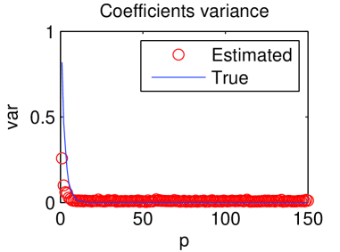
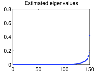
(a) (b)

Figure 1: Component variances and eigenvalues, $m=25$, $n=150$

A simple algorithm is the following:

1. Initiate some small value of $\hat{}\beta_{1},\dots,\hat{}\beta_{n}$. Let $A=\sum_{j=1}^{n}\hat{}\beta_{j}\hat{}\beta_{j}^{\scriptstyle{\mathsf{T}}}$. Fix $\gamma\in(0,1]$, $\varepsilon>0$, $k$, and $c>1$.

2. For $i=1,\dots,n$:

   1. Compute $\delta_{i}=(X_{i}^{\scriptstyle{\mathsf{T}}}X_{i}+\lambda A^{-1/2})^{-1}X_{i}^{\scriptstyle{\mathsf{T}}}(y_{i}-X_{i}\hat{}\beta_{i})$.

   2. Update $A\leftarrow A-\hat{}\beta_{i}\hat{}\beta_{i}$; $\hat{}\beta_{i}\leftarrow\hat{}\beta_{i}+\gamma\delta_{i}$; $A\leftarrow A+\hat{}\beta_{i}\hat{}\beta_{i}$;

3. if $\sum_{j=1}^{p}\mbox{\Large$\mathbf{1}$}\bigl{(}n^{-1}\sum_{i=1}^{n}\hat{}\beta_{ij}^{2}>\varepsilon\bigr{)}>k$ update $\lambda\leftarrow\lambda c$ otherwise $\lambda\leftarrow\lambda/c$.

4. Return to step 2 unless there is no real change of coefficients.

To fasten the computation, the SVD was computed only every 10 values of $i$.

As a simulation we applied the above algorithm to the following simulated data. We generated random $\beta_{1},\dots,\beta_{150}\in{\mathbb{R}}^{150}$ such that all coordinates are independent, and $\beta_{ij}\sim\mathcal{N}(0,e^{-2j/5})$. All $X_{ij\ell}$ are i.i.d. $\mathcal{N}(0,1)$, and $y_{ij}=x_{ij\cdot}^{\scriptstyle{\mathsf{T}}}\beta_{i}+\varepsilon_{ij}$, where $\varepsilon_{ij}$ are all i.i.d. $\mathcal{N}(0,1)$. The true $R^{2}$ obtained was approximately 0.73. The number of replicates per value of $\beta$, $m$, varied between 5 to 300. We consider two measures of estimation error:

$$L_{\rm par} =\frac{\sum_{i=1}^{n}\|\hat{}\beta_{i}-\beta_{i}\|_{\infty}}{\sum_{i=1}^{n}\|\beta_{i}\|_{\infty}}$$

$$L_{\rm pre} =\frac{\sum_{i=1}^{n}\|X_{j}(\hat{}\beta_{i}-\beta_{i})\|_{\infty}}{\sum_{i=1}^{n}\|X_{i}\beta_{i}\|_{\infty}}$$

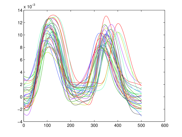
Figure 2: Lower lip position while repeating 32 times ’Say bob again’

The algorithm stopped after 30–50 iterations. Figure is a graphical presentation of a typical result. A summary is given in Table 1. Note that $m$ has a critical impact on the estimation problem. However, with as little as $5$ observations per $R^{150}$ vector of parameter we obtain a significant reduction in the prediction error.

Table 1: The estimation and prediction error as function of the number of observations per vector of parameters Means (and SDK).

$m$	$L_{\rm par}$	$L_{\rm pre}$
5	0.9530 (0.0075)	0.7349 (0.0375)
25	0.7085 (0.0289)	0.7364 (0.0238)
300	0.2470 (0.0080)	0.5207 (0.0179)

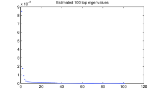
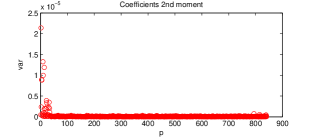
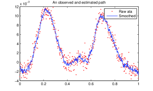
(a) (b) (c)

Figure 3: Eigenvalue, coefficient variance and typical observed and smooth path.

The technique is natural for functional data analysis. We used the data LipPos. The data is described by Ramsay and Silverman and can be found in http://www.stats.ox.ac.uk/ silverma/fdacasebook/lipemg.html. The original data is given in Figure 2. However we added noise to the data as can be seen in Figure 3. The lip position is measured at $m=501$ time points, with $n=32$ repetitions.

As the matrix $X$ we considered the union of 6 cubic spline bases with, respectively, 5, 10, 20, 100, 200, and 500 knots (i.e., $p=841$, and $X_{i}$ does not depend on $i$). A Gaussian noise with $\sigma=0.001$ was added to $Y$. The result of the analysis is given in Figure 3. Figure 4 presents the projection of the mean path on the first eigen-vectors of $\sum_{i=1}^{n}\hat{}\beta_{i}\hat{}\beta_{i}^{\scriptstyle{\mathsf{T}}}$.

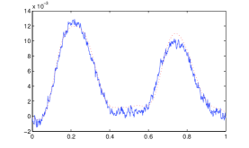
Figure 4: Projection of the estimated mean path on the 2 first eigen-vectors of $\sum_{i=1}^{n}\hat{}\beta_{i}\hat{}\beta_{i}^{\scriptstyle{\mathsf{T}}}$ and the true mean path.

The final example we consider is somewhat arbitrary. The data, taken from StatLib, is of the daily wind speeds for 1961-1978 at 12 synoptic meteorological stations in the Republic of Ireland. As the $Y$ variable we considered one of the stations (station BIR). As explanatory variables we considered the 11 other station of the same day, plus all 12 stations 70 days back (with the constant we have altogether 852 explanatory variables). The analysis was stratified by month. For simplicity, only the first 28 days of the month were taken, and the first year, 1961, served only for explanatory purpose. The last year was served only for testing purpose, so, the training set was for 16 years ($n=12$, $m=448$, and $p=852$ ). In Figure 5 we give the 2nd moments of the coefficients and the scatter plot of predictions vs. true value of the last year.

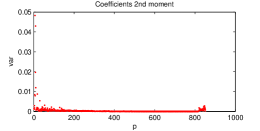
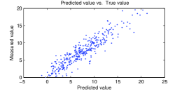
(a) (b)

Figure 5: Coefficient 2nd moment and prediction vs.true value of the test year.

Appendix A Appendix

A.1 General persistence result.

A sequence of estimators $\hat{\beta}^{(m,n,p)}$ is persistent with respect to a set of distributions ${\mathcal{F}}_{n,p}^{m}$ for $\beta\in B_{n,p}$, if for any $F_{m,n,p}\in{\mathcal{F}}_{n,p}^{m}$,

$$L_{F_{m,n,p}}\left(\hat{}\beta^{(m,n,p)}\right)-L_{F_{m,n,p}}\left(\beta^{*}_{F_{m,n,p}}\right)\stackrel{{\scriptstyle P}}{{\rightarrow}}0,$$

where $L_{F}(\beta)=(nm)^{-1}E_{F}\sum_{i=1}^{n}\sum_{j=1}^{m}(Y_{ij}-X_{ij}^{\scriptstyle{\mathsf{T}}}\beta_{i})^{2}$, $F_{m,n,p}$ is the empirical distribution function of $n\times(p+1)$ matrix $Z$, $Z_{i}=(Y_{i},X_{i1},\dots,X_{ip})$, $i=1,\dots,n$, observed $m$ times. Here $\beta^{*}_{F_{m,n,p}}=\mathop{\mathrm{arg\,min}}_{\beta\in B_{n,p}}L_{F_{m,n,p}}(\beta)$, and ${\mathcal{F}}_{n,p}^{m}$ stands for a collection of distributions of $m$ observations of vectors $Z_{i}=(Y_{i},X_{i1},\dots,X_{ip})$, $i=1,\dots,n$.

Assumption F. Under the distributions of random variables $Z$ in ${\mathcal{F}}_{n,p}$, $\xi_{i\ell k}=Z_{i\ell}Z_{ik}$ satisfy $E\left(\max_{i=1,\dots,n}\max_{\ell,k=1,\dots p+1}\xi_{i\ell k}^{2}\right)<V$. Denote this set of distributions by ${\mathcal{F}}_{n,p}(V)$.

This assumption is similar to one of the assumptions of Greenshtein and Ritov (2004). It is satisfied if, for instance, the distribution of $Z_{i\ell}$ has finite support and the variance of $Z_{i\ell}Z_{ik}$ is finite.

Lemma A.1

Let $F\in{\mathcal{F}}_{n,p}(V)$, and denote $\Sigma_{i}=(\sigma_{ijk})$ and $\hat{\Sigma}_{i}=(\hat{\sigma}_{ik\ell})$, with $\sigma_{ijk}=E_{F}Z_{ij}Z_{ik}$ and $\hat{\sigma}_{ik\ell}=m^{-1}\sum_{j=1}^{m}Z_{ik}^{(j)}Z_{i\ell}^{(j)}$, where $Z=(Z_{i\ell}^{(j)})$ is a sample from $F^{m}$, $i=1,\dots,n$, $j=1,\dots,m$, $\ell=1,\dots,p$.

Let $\hat{\beta}$ be the estimator minimising $\sum_{i=1}^{n}\sum_{j=1}^{m}(Y_{ij}-X_{ij}^{\scriptstyle{\mathsf{T}}}\beta_{i})^{2}$ subject to $\beta\in B$ where $B$ is some subset of $\mathbb{R}^{n\times p}$.

Then, for any $\eta\in(0,1)$,

$$\text{(a)\,}\max_{i=1,\dots,n}||\Sigma_{i}-\hat{\Sigma}_{i}||_{\infty} \leqslant \sqrt{\frac{2eV\log(n(p+1)^{2})}{m\,\eta}},$$

$$\text{(b) \,}|L_{F}(\beta)-L_{\hat{F}}(\beta)| \leqslant \frac{1}{nm}\sqrt{\frac{2eV\log(n(p+1)^{2})}{m\eta}}\left(n+\sum_{i=1}^{n}\|\beta_{i}\|_{1}^{2}\right)$$

with probability at least $1-\eta$.

Proof.

Follows that of Theorem 1 in Greenshtein and Ritov (2004).

a) Let $\hat{\sigma}_{ik\ell}=\sigma_{ik\ell}+\epsilon_{ik\ell}$, $E_{i}=(\epsilon_{ik\ell})$. Then, under Assumption F and by Nemirovsky’s inequality (see e.g. Lounici et al [10]),

$$P(\max_{i}||\Sigma_{i}-\hat{\Sigma}_{i}||_{\infty}>A)$$

$$\leqslant\frac{1}{A^{2}}E(\max_{i}||\Sigma_{i}-\hat{\Sigma}_{i}||_{\infty}^{2})$$

$$\leqslant\frac{2e\log(n(p+1)^{2})}{mA^{2}}E(\max_{i=1,\dots,n}\max_{j,k=1,\dots p+1}(Z_{ij}Z_{ik}-E(Z_{ij}Z_{ik}))^{2})$$

$$\leqslant\frac{2eV\log(n(p+1)^{2})}{mA^{2}}.$$

Taking $A=\sqrt{\frac{2eV\log(n(p+1)^{2})}{m\,\eta}}$ proves the first part of the lemma.

b) By the definition of $\hat{\beta}$ and $\beta^{*}_{F}$,

$$L_{F}(\hat{\beta})-L_{{F}}(\beta^{*}_{F})\geqslant 0,\quad L_{\hat{F}}(\hat{\beta})-L_{\hat{F}}(\beta^{*}_{F})\leqslant 0.$$

Hence,

$$0 \leqslant L_{F}\left(\hat{}\beta\right)-L_{F}\left(\beta^{*}_{F}\right)=L_{F}\left(\hat{}\beta\right)-L_{\hat{F}}\left(\hat{}\beta\right)$$

$$+L_{\hat{F}}\left(\hat{}\beta\right)-L_{{F}}\left(\hat{}\beta\right)+L_{{F}}\left(\hat{}\beta\right)-L_{F}\left(\beta^{*}_{F}\right)$$

$$\leqslant 2\sup_{\beta\in B_{n,p}}|L_{F}(\beta)-L_{\hat{F}}(\beta)|.$$

Denote $\delta_{i}^{\scriptstyle{\mathsf{T}}}=(-1,\beta_{i,1},\dots,\beta_{i,p})$, then

$$L_{F}(\beta)=\frac{1}{nm}\sum_{i=1}^{n}\delta_{i}^{\scriptstyle{\mathsf{T}}}\Sigma_{F,i}\delta_{i},$$

where $\Sigma_{F,i}=(\sigma_{ijk})$ and $\sigma_{ijk}=E_{F}Z_{ij}Z_{ik}$. For the empirical distribution function $\hat{F}_{mn}$ determined by a sample $Z_{i\ell}^{(j)}$, $i=1,\dots,n$, $j=1,\dots,m$, $\ell=1,\dots,p$, $\Sigma_{\hat{F},i}=(\hat{\sigma}_{ik\ell})$ and $\hat{\sigma}_{ik\ell}=\frac{1}{m}\sum_{j=1}^{m}Z_{ik}^{(j)}Z_{i\ell}^{(j)}.$

Introduce matrix $\hat{{\mathcal{E}}}$ with $\hat{{\mathcal{E}}}_{j\ell}=A$. Hence, with probability at least $1-\eta$,

$$|L_{F}(\beta)-L_{\hat{F}}(\beta)| =\left|\frac{1}{nm}\sum_{i=1}^{n}\delta_{i}^{\scriptstyle{\mathsf{T}}}(\Sigma_{F,i}-\Sigma_{\hat{F}},i)\delta_{i}\right|$$

$$\leqslant\frac{1}{nm}\sum_{i=1}^{n}|\delta_{i}|^{\scriptstyle{\mathsf{T}}}\hat{{\mathcal{E}}}|\delta_{i}|$$

$$=\frac{1}{nm}\sqrt{\frac{2eV\log(n(p+1)^{2})}{m\eta}}(n+\sum_{i=1}^{n}\|\beta_{i}\|_{1}^{2}).$$

$\square$

A.2 Proofs of Section 2

Proof of Theorem 2.1.

Note that by the definition of $\beta{\tilde{\hat{\vbox to6.94444pt{}}}}\hskip 1.69688pt_{i}$ and 5.

$$\begin{split}\allowdisplaybreaks&mnc_{n}+\lambda_{n}\sum_{i=1}^{n}\|\beta{\tilde{\hat{\vbox to6.94444pt{}}}}\hskip 1.69688pt_{i}\|_{1}^{2}\\ &\leq m\sum_{i=1}^{n}\beta{\tilde{\hat{\vbox to6.94444pt{}}}}\hskip 1.69688pt_{i}^{\scriptstyle{\mathsf{T}}}\tilde{}\Sigma_{i}\beta{\tilde{\hat{\vbox to6.94444pt{}}}}\hskip 1.69688pt_{i}+\lambda_{n}\sum_{i=1}^{n}\|\beta{\tilde{\hat{\vbox to6.94444pt{}}}}\hskip 1.69688pt_{i}\|_{1}^{2}\\ &\leq m\sum_{i=1}^{n}\beta{\tilde{\hat{\vbox to6.94444pt{}}}}\hskip 1.69688pt_{i}^{\scriptstyle{\mathsf{T}}}\tilde{S}_{i}\beta{\tilde{\hat{\vbox to6.94444pt{}}}}\hskip 1.69688pt_{i}+(\lambda_{n}+m\delta_{n})\sum_{i=1}^{n}\|\beta{\tilde{\hat{\vbox to6.94444pt{}}}}\hskip 1.69688pt_{i}\|_{1}^{2}\\ &\leq m\sum_{i=1}^{n}\tilde{}\beta_{i0}^{\scriptstyle{\mathsf{T}}}\tilde{S}_{i}\tilde{}\beta_{i0}+\lambda_{n}\sum_{i=1}^{n}\|\tilde{}\beta_{i0}\|_{1}^{2}+m\delta_{n}\sum_{i=1}^{n}\|\beta{\tilde{\hat{\vbox to6.94444pt{}}}}\hskip 1.69688pt_{i}\|_{1}^{2}\\ &\leq m\sum_{i=1}^{n}\tilde{}\beta_{i0}^{\scriptstyle{\mathsf{T}}}\tilde{}\Sigma_{i}\tilde{}\beta_{i0}+(\lambda_{n}+m\delta_{n})\sum_{i=1}^{n}\|\tilde{}\beta_{i0}\|_{1}^{2}+m\delta_{n}\sum_{i=1}^{n}\|\beta{\tilde{\hat{\vbox to6.94444pt{}}}}\hskip 1.69688pt_{i}\|_{1}^{2}\\ &=mnC_{n}+(\lambda_{n}+m\delta_{n})\sum_{i=1}^{n}\|\tilde{}\beta_{i0}\|_{1}^{2}+m\delta_{n}\sum_{i=1}^{n}\|\beta{\tilde{\hat{\vbox to6.94444pt{}}}}\hskip 1.69688pt_{i}\|_{1}^{2}.\end{split}$$ (13)

Comparing the LHS with the RHS of 13, noting that $m\delta_{n}\ll\lambda_{n}$:

$$\sum_{i=1}^{n}\|\beta{\tilde{\hat{\vbox to6.94444pt{}}}}\hskip 1.69688pt_{i}\|_{1}^{2} \leq mn\frac{C_{n}-c_{n}}{\lambda_{n}-m\delta_{n}}+\frac{\lambda_{n}+m\delta_{n}}{\lambda_{n}-m\delta_{n}}\sum_{i=1}^{n}\|\tilde{}\beta_{i0}\|_{1}^{2}.$$

By 5 and 6:

$$\begin{split}\allowdisplaybreaks\sum_{i=1}^{n}\beta{\tilde{\hat{\vbox to6.94444pt{}}}}\hskip 1.69688pt_{i}^{\scriptstyle{\mathsf{T}}}\tilde{}\Sigma_{i}\beta{\tilde{\hat{\vbox to6.94444pt{}}}}\hskip 1.69688pt_{i}&\leq\sum_{i=1}^{n}\beta{\tilde{\hat{\vbox to6.94444pt{}}}}\hskip 1.69688pt_{i}^{\scriptstyle{\mathsf{T}}}\tilde{S}_{i}\beta{\tilde{\hat{\vbox to6.94444pt{}}}}\hskip 1.69688pt_{i}+\delta_{n}\sum_{i=1}^{n}\|\beta{\tilde{\hat{\vbox to6.94444pt{}}}}\hskip 1.69688pt_{i}\|_{1}^{2}\\ &\leq\sum_{i=1}^{n}\tilde{}\beta_{i0}^{\scriptstyle{\mathsf{T}}}\tilde{S}_{i}\tilde{}\beta_{i0}+\frac{\lambda_{n}}{m}\sum_{i=1}^{n}\|\tilde{}\beta_{i0}\|_{1}^{2}-\frac{\lambda_{n}}{m}\sum_{i=1}^{n}\|\beta{\tilde{\hat{\vbox to6.94444pt{}}}}\hskip 1.69688pt_{i}\|_{1}^{2}+\delta_{n}\sum_{i=1}^{n}\|\beta{\tilde{\hat{\vbox to6.94444pt{}}}}\hskip 1.69688pt_{i}\|_{1}^{2}\\ &\leq\sum_{i=1}^{n}\tilde{}\beta_{i0}^{\scriptstyle{\mathsf{T}}}\tilde{}\Sigma_{i}\tilde{}\beta_{i0}+(\frac{\lambda_{n}}{m}+\delta_{n})\sum_{i=1}^{n}\|\tilde{}\beta_{i0}\|_{1}^{2}-(\frac{\lambda_{n}}{m}-\delta_{n})\sum_{i=1}^{n}\|\beta{\tilde{\hat{\vbox to6.94444pt{}}}}\hskip 1.69688pt_{i}\|_{1}^{2}\\ &\leq\sum_{i=1}^{n}\tilde{}\beta_{i0}^{\scriptstyle{\mathsf{T}}}\tilde{}\Sigma_{i}\tilde{}\beta_{i0}+(\frac{\lambda_{n}}{m}+\delta_{n})\sum_{i=1}^{n}\|\tilde{}\beta_{i0}\|_{1}^{2}.\end{split}$$ (14)

The result follows. $\square$

Proof of Theorem 2.2.

The proof is similar to the proof of Theorem 2.1. Similar to 13 we obtain:

$$\begin{split}\allowdisplaybreaks&mnc_{n}+\lambda_{n}\sum_{i=1}^{n}\|\beta{\tilde{\hat{\vbox to6.94444pt{}}}}\hskip 1.69688pt_{i}\|_{1}^{\alpha}\\ &\leq m\sum_{i=1}^{n}\beta{\tilde{\hat{\vbox to6.94444pt{}}}}\hskip 1.69688pt_{i}^{\scriptstyle{\mathsf{T}}}\tilde{}\Sigma_{i}\beta{\tilde{\hat{\vbox to6.94444pt{}}}}\hskip 1.69688pt_{i}+\lambda_{n}\sum_{i=1}^{n}\|\beta{\tilde{\hat{\vbox to6.94444pt{}}}}\hskip 1.69688pt_{i}\|_{1}^{\alpha}\\ &\leq m\sum_{i=1}^{n}\beta{\tilde{\hat{\vbox to6.94444pt{}}}}\hskip 1.69688pt_{i}^{\scriptstyle{\mathsf{T}}}\tilde{S}_{i}\beta{\tilde{\hat{\vbox to6.94444pt{}}}}\hskip 1.69688pt_{i}+\lambda_{n}\sum_{i=1}^{n}\|\beta{\tilde{\hat{\vbox to6.94444pt{}}}}\hskip 1.69688pt_{i}\|_{1}^{\alpha}+m\delta_{n}\sum_{i=1}^{n}\|\beta{\tilde{\hat{\vbox to6.94444pt{}}}}\hskip 1.69688pt_{i}\|_{1}^{2}\\ &\leq m\sum_{i=1}^{n}\tilde{}\beta_{i0}^{\scriptstyle{\mathsf{T}}}\tilde{S}_{i}\tilde{}\beta_{i0}+\lambda_{n}\sum_{i=1}^{n}\|\tilde{}\beta_{i0}\|_{1}^{\alpha}+m\delta_{n}\sum_{i=1}^{n}\|\beta{\tilde{\hat{\vbox to6.94444pt{}}}}\hskip 1.69688pt_{i}\|_{1}^{2}\\ &\leq m\sum_{i=1}^{n}\tilde{}\beta_{i0}^{\scriptstyle{\mathsf{T}}}\tilde{}\Sigma_{i}\tilde{}\beta_{i0}+\lambda_{n}\sum_{i=1}^{n}\|\tilde{}\beta_{i0}\|_{1}^{\alpha}+m\delta_{n}\sum_{i=1}^{n}\|\tilde{}\beta_{i0}\|_{1}^{2}+m\delta_{n}\sum_{i=1}^{n}\|\beta{\tilde{\hat{\vbox to6.94444pt{}}}}\hskip 1.69688pt_{i}\|_{1}^{2}\\ &=mnc_{n}+\lambda_{n}\sum_{i=1}^{n}\|\tilde{}\beta_{i0}\|_{1}^{\alpha}+m\delta_{n}\sum_{i=1}^{n}\|\tilde{}\beta_{i0}\|_{1}^{2}+m\delta_{n}\sum_{i=1}^{n}\|\beta{\tilde{\hat{\vbox to6.94444pt{}}}}\hskip 1.69688pt_{i}\|_{1}^{2}.\end{split}$$ (15)

That is,

$$\begin{split}\allowdisplaybreaks\sum_{i=1}^{n}(\lambda_{n}\|\beta{\tilde{\hat{\vbox to6.94444pt{}}}}\hskip 1.69688pt_{i}\|_{1}^{\alpha}-m\delta_{n}\|\beta{\tilde{\hat{\vbox to6.94444pt{}}}}\hskip 1.69688pt_{i}\|_{1}^{2})&\leq\lambda_{n}\sum_{i=1}^{n}\|\tilde{}\beta_{i0}\|_{1}^{\alpha}+m\delta_{n}\sum_{i=1}^{n}\|\tilde{}\beta_{i0}\|_{1}^{2}\\ &=\mathcal{O}(mn\delta_{n}).\end{split}$$ (16)

It is easy to see that the maximum of $\sum_{i=1}^{n}\|\beta{\tilde{\hat{\vbox to6.94444pt{}}}}\hskip 1.69688pt_{i}\|_{1}^{2}$ subject to the constraint 16 is achieved when $\|\beta{\tilde{\hat{\vbox to6.94444pt{}}}}\hskip 1.69688pt_{1}\|_{1}^{2}=\dots=\|\beta{\tilde{\hat{\vbox to6.94444pt{}}}}\hskip 1.69688pt_{n}\|_{1}^{2}$. That is when $\|\beta{\tilde{\hat{\vbox to6.94444pt{}}}}\hskip 1.69688pt_{i}\|_{1}^{2}$ solves $\lambda_{n}u^{\alpha}-m\delta_{n}u^{2}=\mathcal{O}(m\delta_{n})$. As $\lambda_{n}=\mathcal{O}(m\delta_{m})$, the solution satisfies $u=\mathcal{O}(m\delta_{n}/\lambda_{n})^{1/(\alpha-2)}$.

Hence we can conclude from 16

$$\sum_{i=1}^{n}\|\beta{\tilde{\hat{\vbox to6.94444pt{}}}}\hskip 1.69688pt_{i}\|_{2}^{2} =\mathcal{O}(n(m\delta_{n}/\lambda_{n})^{2/(\alpha-2)})$$

We now proceed similar to 14

$$\sum_{i=1}^{n}\beta{\tilde{\hat{\vbox to6.94444pt{}}}}\hskip 1.69688pt_{i}^{\scriptstyle{\mathsf{T}}}\tilde{}\Sigma_{i}\beta{\tilde{\hat{\vbox to6.94444pt{}}}}\hskip 1.69688pt_{i} \leq\sum_{i=1}^{n}\beta{\tilde{\hat{\vbox to6.94444pt{}}}}\hskip 1.69688pt_{i}^{\scriptstyle{\mathsf{T}}}\tilde{S}_{i}\tilde{}\beta_{i}+\delta_{n}\sum_{i=1}^{n}\|\beta{\tilde{\hat{\vbox to6.94444pt{}}}}\hskip 1.69688pt_{i}\|_{1}^{2}$$

$$\leq\sum_{i=1}^{n}\tilde{}\beta_{i0}^{\scriptstyle{\mathsf{T}}}\tilde{S}_{i}\tilde{}\beta_{i0}+\frac{\lambda_{n}}{m}\sum_{i=1}^{n}\|\tilde{}\beta_{i0}\|_{1}^{\alpha}-\frac{\lambda_{n}}{m}\sum_{i=1}^{n}\|\beta{\tilde{\hat{\vbox to6.94444pt{}}}}\hskip 1.69688pt_{i}\|_{1}^{\alpha}+\delta_{n}\sum_{i=1}^{n}\|\beta{\tilde{\hat{\vbox to6.94444pt{}}}}\hskip 1.69688pt_{i}\|_{1}^{2}$$

$$\leq\sum_{i=1}^{n}\tilde{}\beta_{i0}^{\scriptstyle{\mathsf{T}}}\tilde{}\Sigma_{i}\tilde{}\beta_{i0}+\frac{\lambda_{n}}{m}\sum_{i=1}^{n}\|\tilde{}\beta_{i0}\|_{1}^{\alpha}+\delta_{n}\sum_{i=1}^{n}\|\tilde{}\beta_{i0}\|_{1}^{2}+\delta_{n}\sum_{i=1}^{n}\|\beta{\tilde{\hat{\vbox to6.94444pt{}}}}\hskip 1.69688pt_{i}\|_{1}^{2}$$

$$\leq\sum_{i=1}^{n}\tilde{}\beta_{i0}^{\scriptstyle{\mathsf{T}}}\tilde{}\Sigma_{i}\tilde{}\beta_{i0}+\mathcal{O}_{p}(n(m/\lambda_{n})^{2/(\alpha-2)}\delta_{n}^{\alpha/(\alpha-2)}),$$

since $\lambda_{n}=\mathcal{O}(m\delta_{m})$.

$\square$

Proof of Remark 2.1.

If $m\delta_{m}/\lambda=\text{$\mathcal{O}$}(1)$, then, following the proof of Theorem 2.2, the solution maximising $\sum_{i=1}^{n}\|\beta{\tilde{\hat{\vbox to6.94444pt{}}}}\hskip 1.69688pt_{i}\|_{1}^{2}$ subject to the constraint 16 satisfies $\|\beta{\tilde{\hat{\vbox to6.94444pt{}}}}\hskip 1.69688pt_{i}\|_{1}=\mathcal{O}(1)$, and hence we have

$$\sum_{i=1}^{n}\beta{\tilde{\hat{\vbox to6.94444pt{}}}}\hskip 1.69688pt_{i}^{\scriptstyle{\mathsf{T}}}\tilde{}\Sigma_{i}\beta{\tilde{\hat{\vbox to6.94444pt{}}}}\hskip 1.69688pt_{i} \leq\sum_{i=1}^{n}\tilde{}\beta_{i0}^{\scriptstyle{\mathsf{T}}}\tilde{}\Sigma_{i}\tilde{}\beta_{i0}+\mathcal{O}_{p}\left(n\lambda_{n}/m+n\delta_{n}\right).$$

$\square$

Proof of Theorem 2.3.

The proof follows that of Lemma 3.1 in Lounici et al. [10].

We start with (a) and (b). Since $\hat{}\beta$ minimizes 6, then, $\forall\beta$

$$\sum_{i=1}^{n}||Y_{i}-X_{i}^{\scriptstyle{\mathsf{T}}}\hat{}\beta_{i}||_{2}^{2}+\lambda\sum_{i=1}^{n}\|\hat{}\beta_{i}\|_{1}^{\alpha} \leq\sum_{i=1}^{n}||Y_{i}-X_{i}^{\scriptstyle{\mathsf{T}}}\beta_{i}||_{2}^{2}+\lambda\sum_{i=1}^{n}\|\beta_{i}\|_{1}^{\alpha},$$

and hence, for $Y_{i}=X_{i}^{\scriptstyle{\mathsf{T}}}\beta_{i}+\varepsilon_{i}$,

$$\sum_{i=1}^{n}||X_{i}^{\scriptstyle{\mathsf{T}}}(\hat{}\beta_{i}-\beta_{i})||_{2}^{2}\leqslant\sum_{i=1}^{n}\left[2\varepsilon_{i}^{\scriptstyle{\mathsf{T}}}X_{i}^{\scriptstyle{\mathsf{T}}}(\beta_{i}-\hat{}\beta_{i})+\lambda(||\beta_{i}||_{1}^{\alpha}-||\hat{}\beta_{i}||_{1}^{\alpha})\right].$$

Denote $V_{i\ell}=\sum_{j=1}^{m}x_{ij\ell}\varepsilon_{ij}\sim\mathcal{N}(0,m\sigma^{2})$, and introduce event ${\mathcal{A}}_{i}=\bigcap_{\ell=1}^{p}\{|V_{i\ell}|\leq\mu\}$, for some $\mu>0$. Then

$$P({\mathcal{A}}_{i}^{c}) \leq\sum_{\ell=1}^{p}P(|V_{i\ell}|>\mu)$$

$$=\sum_{\ell=1}^{p}2\biggl{[}1-\Phi\Bigl{\{}\mu/(\sigma\sqrt{m})\Bigr{\}}\biggr{]}$$

$$\leq p\exp\bigl{\{}-\mu^{2}/(2m\sigma^{2})\bigr{\}}.$$

For ${\mathcal{A}}=\cap_{i=1}^{n}{\mathcal{A}}_{i}$, due to independence,

$$P({\mathcal{A}}^{c})=\sum_{i=1}^{n}P({\mathcal{A}}_{i}^{c})\leqslant pn\exp\bigl{\{}-\mu^{2}/(2m\sigma^{2})\bigr{\}}.$$

Thus, if $\mu$ is large enough, $P({\mathcal{A}}^{c})$ is small, e.g., for $\mu=\sigma A\bigl{(}m\log(np)\bigr{)}^{1/2}$, $A>\sqrt{2}$, we have $P({\mathcal{A}}^{c})\leq(np)^{1-A^{2}/2}$.

On event ${\mathcal{A}}$, for some $\nu>0$,

$$\sum_{i=1}^{n}\left[||X_{i}(\hat{}\beta_{i}-\beta_{i})||_{2}^{2}+\nu||\beta_{i}-\hat{}\beta_{i}||_{1}\right]$$

$$\leqslant\sum_{i=1}^{n}\left[2\mu||\beta_{i}-\hat{}\beta_{i}||_{1}+\lambda(||\beta_{i}||_{1}^{2}-||\hat{}\beta_{i}||_{1}^{2})\right.+\left.\nu||\beta_{i}-\hat{}\beta_{i}||_{1}\right]$$

$$=\sum_{i=1}^{n}\sum_{j=1}^{m}\left[\alpha\,\lambda\max(||\beta_{i}||_{1}^{\alpha-1},||\hat{}\beta_{i}||_{1}^{\alpha-1})(|\beta_{ij}|-|\hat{}\beta_{ij}|)+(\nu+2\mu)|\beta_{ij}-\hat{}\beta_{ij}|\right]$$

$$\leqslant\sum_{i=1}^{n}\sum_{j=1}^{m}\left[\alpha\,\lambda\max(B^{\alpha-1},\hat{B}^{\alpha-1})(|\beta_{ij}|-|\hat{}\beta_{ij}|)+(\nu+2\mu)|\beta_{ij}-\hat{}\beta_{ij}|\right],$$

due to inequality $|x^{\alpha}-y^{\alpha}|\leqslant\alpha|x-y|\max(|x|^{\alpha-1},|y|^{\alpha-1})$ which holds for $\alpha\geqslant 1$ and any $x$ and $y$. To simplify the notation, denote ${\mathcal{C}}=\alpha\,\max(B^{\alpha-1},\hat{B}^{\alpha-1})$.

Denote $J_{i}=J(\beta_{i})=\{j:\,\,\beta_{ij}\neq 0\}$, ${\mathcal{M}}(\beta_{i})=|J(\beta_{i})|$. For each $i$ and $j\in J(\beta_{i})$, the expression in square brackets is bounded above by

$$[\lambda{\mathcal{C}}+\nu+2\mu]\,|\beta_{ij}-\hat{}\beta_{ij}|,$$

and for $j\in J^{c}(\beta)$, the expression in square brackets is bounded above by $0$, as long as $\nu+2\mu\leqslant\lambda{\mathcal{C}}$:

$$-\lambda{\mathcal{C}}|\hat{}\beta_{ij}|+(\nu+2\mu)|\hat{}\beta_{ij}|\leqslant 0.$$

This condition is satisfied if $\nu+2\mu\leqslant\lambda{\mathcal{C}}$.

Hence, on ${\mathcal{A}}$, for $\nu+2\mu\leqslant\lambda{\mathcal{C}}$,

$$\sum_{i=1}^{n}\left[||X_{i}^{\scriptstyle{\mathsf{T}}}(\hat{}\beta_{i}-\beta_{i})||_{2}^{2}+\nu||\beta_{i}-\hat{}\beta_{i}||_{1}\right]\leqslant\sum_{i=1}^{n}[\lambda{\mathcal{C}}+2\mu+\nu]||(\beta_{i}-\hat{}\beta_{i})_{J_{i}}||_{1}.$$

This implies that

$$\sum_{i=1}^{n}||X_{i}(\hat{}\beta_{i}-\beta_{i})||_{2}^{2}\leqslant[\lambda{\mathcal{C}}+\nu+2\mu]||(\beta-\hat{}\beta)_{J}||_{1},$$

as well as that

$$||\beta-\hat{}\beta||_{1}\leqslant\left[1+\frac{2\mu}{\nu}+\frac{\lambda}{\nu}{\mathcal{C}}\right]||(\beta-\hat{}\beta)_{J}||_{1}.$$

Take $\nu=\lambda{\mathcal{C}}/2$, hence we need to assume that $2\mu\leqslant\lambda{\mathcal{C}}/2$:

$$\begin{split}\allowdisplaybreaks\sum_{i=1}^{n}||X_{i}^{\scriptstyle{\mathsf{T}}}(\hat{}\beta_{i}-\beta_{i})||_{2}^{2}&\leqslant\left[\frac{3\lambda}{2}{\mathcal{C}}+2\mu\right]||(\beta-\hat{}\beta)_{J}||_{1},\\ ||\beta-\hat{}\beta||_{1}&\leqslant\left[3+\frac{4\mu}{\lambda{\mathcal{C}}}\right]||(\beta-\hat{}\beta)_{J}||_{1}\leqslant 4||(\beta-\hat{}\beta)_{J}||_{1}.\end{split}$$ (17)

which implies

$$||(\beta-\hat{}\beta)_{J^{c}}||_{1}\leqslant 3||(\beta-\hat{}\beta)_{J}||_{1}.$$

Due to the generalized restricted eigenvalue assumption RE${}_{1}(s,3,\kappa)$, $||X^{\scriptstyle{\mathsf{T}}}(\beta-\hat{}\beta)||_{2}\geqslant\kappa\sqrt{m}||(\beta-\hat{}\beta)_{J}||_{2}$, and hence, using 17,

$$||X^{\scriptstyle{\mathsf{T}}}(\hat{}\beta-\beta)||_{2}^{2} \leqslant\left[\frac{3\lambda}{2}{\mathcal{C}}+2\mu\right]\sqrt{n{\mathcal{M}}(\beta)}||(\hat{}\beta-\beta)_{J}||_{2}$$

$$\leqslant\left[\frac{3\lambda}{2}{\mathcal{C}}+2\mu\right]\frac{\sqrt{n{\mathcal{M}}(\beta)}}{\kappa\sqrt{m}}||X^{\scriptstyle{\mathsf{T}}}(\hat{}\beta-\beta)||_{2},$$

where ${\mathcal{M}}(\beta)=\max_{i}{\mathcal{M}}(\beta_{i})$, implying that

$$||X^{\scriptstyle{\mathsf{T}}}(\hat{}\beta-\beta)||_{2} \leqslant\left[\frac{3\lambda}{2}{\mathcal{C}}+2\mu\right]\frac{\sqrt{n{\mathcal{M}}(\beta)}}{\kappa\sqrt{m}}$$

$$=\frac{\sqrt{n{\mathcal{M}}(\beta)}}{\kappa\sqrt{m}}\left[\frac{3\lambda}{2}{\mathcal{C}}+2A\sigma\sqrt{m\log(np)}\right].$$

Also,

$$||\beta-\hat{}\beta||_{1} \leqslant 4||(\beta-\hat{}\beta)_{J}||_{1}\leqslant 4\frac{\sqrt{n{\mathcal{M}}(\beta)}}{\sqrt{m}\kappa}||X^{\scriptstyle{\mathsf{T}}}(\beta-\hat{}\beta)||_{2}$$

$$\leqslant\frac{4n{\mathcal{M}}(\beta)}{m\kappa^{2}}\left[\frac{3\lambda}{2}{\mathcal{C}}+2A\sigma\sqrt{m\log(np)}\right].$$

Hence, a) and b) of the theorem are proved.

(c) For $i$, $\ell$: $\hat{}\beta_{i\ell}\neq 0$, we have

$$2X_{i\cdot\ell}(Y_{i}-X_{i}^{\scriptstyle{\mathsf{T}}}\hat{}\beta_{i}) =\lambda\alpha{\rm{sgn}\;}(\hat{}\beta_{i\ell})||\hat{}\beta_{i}||_{1}^{\alpha-1}\,,$$

Hence,

$$\sum_{\ell:\,\hat{}\beta_{i\ell}\neq 0}||X_{i\cdot\ell}X_{i}^{\scriptstyle{\mathsf{T}}}(\beta_{i}-\hat{}\beta_{i})||_{2}^{2} \geqslant\sum_{\ell:\,\hat{}\beta_{i\ell}\neq 0}\left(||X_{i\cdot\ell}(Y_{i}-X_{i}^{\scriptstyle{\mathsf{T}}}\hat{}\beta_{i})||_{2}-||X_{i\cdot\ell}(Y_{i}-X_{i}^{\scriptstyle{\mathsf{T}}}\beta_{i})||_{2}\right)^{2}$$

$$\geq\sum_{\ell:\hat{}\beta_{i\ell}\neq 0}\Bigl{(}\alpha\,\lambda||\hat{}\beta_{i}||_{1}^{\alpha-1}/2-\mu\Bigr{)}^{2}$$

$$={\mathcal{M}}(\hat{}\beta_{i})(\alpha\,\lambda||\hat{}\beta_{i}||_{1}^{\alpha-1}/2-\mu)^{2}.$$

Thus,

$${\mathcal{M}}(\hat{}\beta_{i}) \leq\|X_{i}(\beta_{i}-\hat{}\beta_{i})\|_{2}^{2}\frac{m\phi_{i,\,\max}}{\left(\lambda\alpha||\hat{}\beta_{i}||_{1}^{\alpha-1}/2-\mu\right)^{2}}.$$

Theorem is proved. $\square$

Proof of Theorem 2.4..

To satisfy the conditions of Theorem 2.3, we can take $B=b$ and $\lambda=\frac{4A\sigma}{\alpha b^{\alpha-1}}\sqrt{m\log(np)}$.

Thus, by Lemma A.1,

$$\frac{\lambda}{m\delta_{n}}=\frac{4A\sigma}{\alpha b^{\alpha-1}}\sqrt{\frac{\log(np)}{m}}\sqrt{\frac{m\,\eta}{2eV\log(n(p+1)^{2})}}=C\frac{\sqrt{\eta}}{\alpha b^{\alpha-1}}\leqslant C_{1},$$

hence assumption $\lambda=\mathcal{O}(m\delta_{n})$ of Theorem 2.2 is satisfied.

Hence, from the proof of Theorem 2.3, it follows that

$$\|\hat{}\beta_{i}\|_{1} =\mathcal{O}\left((m\delta_{n}/\lambda_{n})^{1/(\alpha-2)}\right)=\mathcal{O}\left(\left(\frac{b^{\alpha-1}}{\sqrt{\eta}}\right)^{1/(\alpha-2)}\right).$$

Hence, we can take $B=b$ and $\hat{B}=C\left(\frac{b^{\alpha-1}}{\sqrt{\eta}}\right)^{1/(\alpha-2)}$ for some $C>0$, and apply Theorem 2.3. Then $\max(1,\hat{B}/B)$ is bounded by

$$\max\left[1,C\frac{b^{(\alpha-1)/(\alpha-2)-1}}{\eta^{1/(2(\alpha-2))}}\right]=\max\left[1,C\frac{b^{1/(\alpha-2)}}{\eta^{1/(2(\alpha-2))}}\right]=\left(\frac{Cb}{\sqrt{\eta}}\right)^{1/(\alpha-2)},$$

since $\frac{Cb}{\sqrt{\eta}}\geqslant C_{2}\frac{\eta^{1/(2(\alpha-1))}}{\sqrt{\eta}}\geqslant C_{2}\eta^{-(\alpha-2)/(2(\alpha-1))}$ is large for small $\eta$.

Hence,

$$\frac{3\alpha\lambda}{2\sqrt{m}}\max(B^{\alpha-1},\hat{B}^{\alpha-1})+2A\sigma\sqrt{\log(np)}$$

$$\leqslant 6AC\sigma\sqrt{\log(np)}\frac{b^{(\alpha-1)/(\alpha-2)}}{\eta^{(\alpha-1)/(2(\alpha-2))}}+2A\sigma\sqrt{\log(np)}$$

$$=2A\sigma\sqrt{\log(np)}\left[3C\left(\frac{b}{\sqrt{\eta}}\right)^{(\alpha-1)/(\alpha-2)}+1\right],$$

and, applying Theorem 2.3, we obtain (a) and (b).

c) Apply c) in Theorem 2.3, summing over $i\in{\mathcal{I}}$:

$$\sum_{i\in{\mathcal{I}}}{\mathcal{M}}(\hat{}\beta_{i}) \leq\|X^{\scriptstyle{\mathsf{T}}}(\beta-\hat{}\beta)\|_{2}^{2}\frac{m\phi_{\max}}{(\mu\delta)^{2}}$$

$$\leq\frac{4sn\phi_{\max}}{\kappa^{2}\,\delta^{2}}\left[1+3C\left(\frac{b}{\sqrt{\eta}}\right)^{(\alpha-1)/(\alpha-2)}\right]^{2}.$$

$\square$

A.3 Proofs of Section 4

Proof of Lemma 4.1.

Let ${\mathcal{B}}=\sum_{\xi=1}^{k}\alpha_{\xi}\beta_{\xi}^{*}{\mathfrak{b}_{\xi}^{*}}^{\scriptstyle{\mathsf{T}}}$ be the spectral decomposition of ${\mathcal{B}}$, where $\beta_{1}^{*},\dots,\beta_{k}^{*}$ are orthonormal ${\mathbb{R}}^{p}$ vectors, $\mathfrak{b}_{1}^{*},\dots,\mathfrak{b}_{k}^{*}$ are orthonormal ${\mathbb{R}}^{n}$ vectors, $\alpha_{1},\dots,\alpha_{k}\geq 0$, and $k=\min\{p,n\}$. Clearly $|||{\mathcal{B}}|||_{1}=\sum_{\xi=1}^{k}\alpha_{\xi}$. Let $U=\sum_{\xi=1}^{k}e_{\xi}{\beta_{\xi}^{*}}^{\scriptstyle{\mathsf{T}}}$ where $e_{1},\dots,e_{p}$ is the natural basis of ${\mathbb{R}}^{n}$. Then

$$\|U{\mathcal{B}}\|_{2,1} =\|\sum_{\xi=1}^{k}\alpha_{\xi}e_{\xi}{\mathfrak{b}_{\xi}^{*}}^{\scriptstyle{\mathsf{T}}}\|_{2,1}=\sum_{\xi=1}^{k}\alpha_{\xi}=|||{\mathcal{B}}|||_{1}.$$

Let ${\mathcal{B}}=\sum_{\xi=1}^{k}e_{\xi}\mathfrak{b}_{\xi}^{\scriptstyle{\mathsf{T}}}$ where $\mathfrak{b}_{1},\mathfrak{b}_{2},\dots,\mathfrak{b}_{k}$ are orthogonal, and let $U$ be a unitary matrix. Then by Schwarz inequality

$$\|{\mathcal{B}}\|_{2,1} =\sum_{j=1}^{p}\|\mathfrak{b}_{j}\|$$

$$=\sum_{i=1}^{p}\sum_{j=1}^{p}U_{ij}^{2}\|\mathfrak{b}_{j}\|\qquad \text{since}\sum_{i=1}^{p}U_{ij}^{2}=1$$

$$\leq\sum_{i=1}^{p}\sqrt{\sum_{j=1}^{p}U_{ij}^{2}\|\mathfrak{b}_{j}\|^{2}}\sqrt{\sum_{j=1}^{p}U_{ij}^{2}}\qquad$$ by Schwarz inequality

$$=\sum_{i=1}^{p}\sqrt{\sum_{j=1}^{p}U_{ij}^{2}\|\mathfrak{b}_{j}\|^{2}}\qquad \text{since}\sum_{j=1}^{p}U_{ij}^{2}=1$$

$$=\|U{\mathcal{B}}\|_{2,1}$$

which completes the proof of the (i).

Now, consider the $U$ defined as above for the solution of 12. Let $\tilde{X}_{i}$ be the design matrices $\tilde{}{\mathcal{B}}$ be the solution expressed in this basis. By the first part of the lemma $|||\tilde{}{\mathcal{B}}|||_{1}=\|\tilde{}{\mathcal{B}}\|_{2,1}$. Suppose there is a matrix ${\mathcal{B}}\neq\tilde{}{\mathcal{B}}$ which minimizes the group lasso penalty. Hence

$$\sum_{i=1}^{n}\|Y_{i}-\tilde{X}_{i}\beta_{i}\|^{2}+\lambda|||{\mathcal{B}}|||_{1} \leq\sum_{i=1}^{n}\|Y_{i}-\tilde{X}_{i}\beta_{i}\|^{2}+\lambda\|{\mathcal{B}}\|_{2,1}$$

$$<\sum_{i=1}^{n}\|Y_{i}-\tilde{X}_{i}\tilde{}\beta_{i}\|^{2}+\lambda\|\tilde{}{\mathcal{B}}\|_{2,1}$$

$$=\sum_{i=1}^{n}\|Y_{i}-\tilde{X}_{i}\tilde{}\beta_{i}\|^{2}+\lambda|||\tilde{}{\mathcal{B}}|||_{1},$$

contradiction since $\tilde{}{\mathcal{B}}$ minimized 12. Part (ii) is proved. $\square$

Proof of Theorem 4.2 .

Let $A=\sum_{i=1}^{n}\hat{}\beta_{i}\hat{}\beta_{i}^{\scriptstyle{\mathsf{T}}}=\hat{}{\mathcal{B}}\hat{}{\mathcal{B}}^{\scriptstyle{\mathsf{T}}}$ be of rank $s\leqslant p<n$, and hence the spectral decomposition of $\hat{}{\mathcal{B}}$ can be written as $\hat{}{\mathcal{B}}=\sum_{\xi=1}^{s}\alpha_{\xi}\beta_{\xi}^{*}{\mathfrak{b}_{\xi}^{*}}^{\scriptstyle{\mathsf{T}}}$, where $\beta_{1}^{*},\dots,\beta_{s}^{*}\in\mathbb{R}^{p}$ are orthonormal, and so are $\mathfrak{b}_{1}^{*},\dots,\mathfrak{b}_{s}^{*}\in\mathbb{R}^{n}$. Hence, the rotation $U$ leading to a sparse representation $U\hat{}{\mathcal{B}}$ (with $s$ non-zero rows) is given by $U=\sum_{\xi=1}^{s}e_{\xi}{\beta_{\xi}^{*}}^{\scriptstyle{\mathsf{T}}}$, where $e_{1},\dots,e_{p}$ is the natural basis of ${\mathbb{R}}^{p}$. Another way to write the rotation matrix is $U=({\beta_{1}^{*}}^{\scriptstyle{\mathsf{T}}},\dots,{\beta_{s}^{*}}^{\scriptstyle{\mathsf{T}}},\mathbf{0}^{\scriptstyle{\mathsf{T}}},\dots,\mathbf{0}^{\scriptstyle{\mathsf{T}}})^{\scriptstyle{\mathsf{T}}}$. Denote by $U_{S}$ the non-zero $s\times p$-dimensional submatrix $({\beta_{1}^{*}}^{\scriptstyle{\mathsf{T}}},\dots,{\beta_{s}^{*}}^{\scriptstyle{\mathsf{T}}})^{\scriptstyle{\mathsf{T}}}$.

Let $A(t)=A+t(\tilde{}\beta\hat{}\beta_{i}^{\scriptstyle{\mathsf{T}}}+\hat{}\beta_{i}\tilde{}\beta^{\scriptstyle{\mathsf{T}}})+t^{2}\tilde{}\beta\tilde{}\beta^{\scriptstyle{\mathsf{T}}}$ for some fixed $i$, with $\tilde{}\beta\in\mathop{\rm span}\nolimits\{\hat{}\beta_{1},\dots,\hat{}\beta_{n}\}=\mathop{\rm span}\nolimits\{\hat{}\beta_{1}^{*},\dots,\hat{}\beta_{s}^{*}\}$.

If $(x_{k}(t),c_{k}(t))$ is an eigen-pair of $A(t)$, then taking the derivative of $x_{i}^{\scriptstyle{\mathsf{T}}}x_{i}=1$ yields $x_{i}^{\scriptstyle{\mathsf{T}}}\dot{x}_{i}=0$, and trivially, since $x_{i}$ is an eigenvector, also $x_{i}^{\scriptstyle{\mathsf{T}}}A\dot{x}_{i}=0$. Here $\dot{}$ and $\ddot{}$ the first and second derivative, respectively, according to $t$. Also, we have

$$x_{k}(t) =x_{k}+tu_{k}+\text{$\mathcal{O}$}(t)$$

$$c_{k}(t) =c_{k}+t\nu_{k}+\text{$\mathcal{O}$}(t)$$

and

$$\Bigl{(}A+t(\tilde{}\beta\hat{}\beta_{i}^{\scriptstyle{\mathsf{T}}}+\hat{}\beta_{i}\tilde{}\beta^{\scriptstyle{\mathsf{T}}})\Bigr{)}(x_{k}+tu_{k}) =(c_{k}+t\nu_{k})(x_{k}+tu_{k})+\text{$\mathcal{O}$}(t),$$

where $u_{k}\perp x_{k}$.

Equating the $\mathcal{O}(t)$ terms obtain

$$Au_{k}+(\tilde{}\beta\hat{}\beta_{i}^{\scriptstyle{\mathsf{T}}}+\hat{}\beta_{i}\tilde{}\beta^{\scriptstyle{\mathsf{T}}})x_{k} =c_{k}u_{k}+\nu_{k}x_{k}.$$

Take now the inner product of both sides with $x_{k}$ to obtain that

$$\begin{split}\allowdisplaybreaks\nu_{k}=2(\tilde{}\beta^{\scriptstyle{\mathsf{T}}}x_{k})(x_{k}^{\scriptstyle{\mathsf{T}}}\hat{}\beta_{i}).\end{split}$$ (18)

Note that the null space of $A(t)$ does not depend on $t$. Hence, if we call $\psi({\mathcal{B}})=|||{\mathcal{B}}|||_{1}$,

$$\frac{\partial}{\partial t}\psi(A(t))|_{t=0} =\sum_{c_{k}>0}\frac{\partial}{\partial t}c_{k}^{1/2}(t)|_{t=0}$$

$$=\frac{1}{2}\sum_{c_{k}>0}\frac{\nu_{k}}{c_{k}^{1/2}}$$

$$=\tilde{}\beta^{\scriptstyle{\mathsf{T}}}\sum_{c_{k}>0}c_{k}^{-1/2}x_{k}x_{k}^{\scriptstyle{\mathsf{T}}}\hat{}\beta_{i}$$

$$=\tilde{}\beta^{\scriptstyle{\mathsf{T}}}A^{+1/2}\hat{}\beta_{i}=\tilde{}\beta^{\scriptstyle{\mathsf{T}}}(\hat{}{\mathcal{B}}\hat{}{\mathcal{B}}^{\scriptstyle{\mathsf{T}}})^{+1/2}\hat{}\beta_{i}$$

$$=\tilde{}\beta^{\scriptstyle{\mathsf{T}}}U_{S}^{\scriptstyle{\mathsf{T}}}(U_{S}\hat{}{\mathcal{B}}\hat{}{\mathcal{B}}^{\scriptstyle{\mathsf{T}}}U_{S}^{\scriptstyle{\mathsf{T}}})^{-1/2}U_{S}\hat{}\beta_{i},$$

where $A^{+1/2}$ is the generalized inverse of $A^{1/2}$.

Taking, therefore, the derivative of the target function with respect to $\hat{}\beta_{i}$ in the directions of $\tilde{}\beta\in\mathop{\rm span}\nolimits\{\hat{}\beta_{1},\dots,\hat{}\beta_{n}\}$ (e.g., in the directions $\tilde{}\beta=\beta_{\xi}^{*}$, $\xi=1,\dots,s$) gives

$$0 =(\beta_{\xi}^{*})^{\scriptstyle{\mathsf{T}}}(-2X_{i}^{\scriptstyle{\mathsf{T}}}(Y_{i}-X_{i}\hat{}\beta_{i})+\lambda(\hat{}{\mathcal{B}}\hat{}{\mathcal{B}}^{\scriptstyle{\mathsf{T}}})^{+1/2}\hat{}\beta_{i}),\quad\text{or, equivalently,}$$

$$\mathbf{0} =U_{S}(2X_{i}^{\scriptstyle{\mathsf{T}}}(Y_{i}-X_{i}\hat{}\beta_{i})-\lambda(\hat{}{\mathcal{B}}\hat{}{\mathcal{B}}^{\scriptstyle{\mathsf{T}}})^{+1/2}\hat{}\beta_{i}).$$

Let $R=(r_{1},\dots,r_{p})^{\scriptstyle{\mathsf{T}}}$ be the matrix of projected residuals:

$$R_{\ell i}=\sum_{j=1}^{m}x_{ij\ell}(y_{ij}-x_{ij}^{\scriptstyle{\mathsf{T}}}\hat{}\beta_{i}),\quad\ell=1,\dots,p\,;\;i=1,\dots,n.$$

Then

$$U_{S}R =\frac{\lambda}{2}U_{S}(\hat{}{\mathcal{B}}\hat{}{\mathcal{B}}^{\scriptstyle{\mathsf{T}}})^{+1/2}\hat{}{\mathcal{B}}.$$

Consider again the general expansion $\hat{}{\mathcal{B}}=\sum_{\xi=1}^{p\wedge n}\alpha_{\xi}\beta_{\xi}^{*}{\mathfrak{b}_{\xi}^{*}}^{\scriptstyle{\mathsf{T}}}$. Then $|||\hat{}{\mathcal{B}}|||_{1}=\sum_{\xi=1}^{p\wedge n}|\alpha_{\xi}|$. Taking the derivative of the sum of squares part of the target function with respect to $\alpha_{\xi}$ we get

$$\sum_{i=1}^{n}\mathfrak{b}^{*}_{\xi i}{\beta^{*}_{\xi}}^{\scriptstyle{\mathsf{T}}}X_{i}^{\scriptstyle{\mathsf{T}}}(Y_{i}-X_{i}\hat{}\beta_{i}) ={\beta_{\xi}^{*}}^{\scriptstyle{\mathsf{T}}}R\mathfrak{b}_{\xi}^{*}.$$

Considering the sub-gradient of the target function we obtain that $|{\beta_{\xi}^{*}}^{\scriptstyle{\mathsf{T}}}R\mathfrak{b}_{\xi}^{*}|\leq\lambda/2$, and $\alpha_{\xi}=0$ in case of strict inequality.

$\square$

Proof of Theorem 4.3 .

(a) and (b) Similarly to the proof of Theorem 2.3, we have

$$\|Y-X^{\scriptstyle{\mathsf{T}}}\hat{}{\mathcal{B}}\|_{2}^{2} =\|Y-X^{\scriptstyle{\mathsf{T}}}{\mathcal{B}}\|_{2}^{2}+2\sum_{ij}\varepsilon_{ij}x_{ij}^{\scriptstyle{\mathsf{T}}}(\beta_{i}-\hat{}\beta_{i}).$$

The last term can be bounded with high probability. Introduce matrix $M$ with independent columns $M_{i}=X_{i}\varepsilon_{i}\sim{\mathcal{N}}_{p}(\mathbf{0},m\sigma^{2}I_{p})$, $i=1,\dots,n$, since $\sum_{j}x_{ij\ell}^{2}=m$. Denote $q$-Schatten norm by $|||\cdot|||_{q}$. Using the Cauchy-Swartz inequality and the equivalence between $\ell_{2}$ (Frobenius) and Schatten with $q=2$ norms, we obtain:

$$|\sum_{ij}\varepsilon_{ij}x_{ij}^{\scriptstyle{\mathsf{T}}}(\beta_{i}-\hat{}\beta_{i})| =|\sum_{i\ell}M_{i\ell}(\beta_{i\ell}-\hat{}\beta_{i\ell})|\leqslant||{\mathcal{B}}-\hat{}{\mathcal{B}}||_{2}\,||M||_{2}=|||{\mathcal{B}}-\hat{}{\mathcal{B}}|||_{2}\,||M||_{2}$$

$$\leqslant|||{\mathcal{B}}-\hat{}{\mathcal{B}}|||_{1}\,||M||_{2}.$$

Now, $||M||_{2}^{2}\sim m\sigma^{2}\chi^{2}_{np}$ hence it can be bounded by $B^{2}=m\sigma^{2}(np+c)$ (Lemma A.1, Lounici et al. [10]) with probability at least $1-\exp\left(-\frac{1}{8}\min(c,c^{2}/(np))\right)$. Denote this event by ${\mathcal{A}}$. Hence, we need to choose $c$ such that $c/\sqrt{np}\to\infty$. For example, we can take $c=Anp$ with $A>1$, then $B=\sigma\sqrt{(1+A)mnp}$, and, since $\min(Anp,A^{2}np)=Anp$, the probability is at least $1-e^{-Anp/2}$.

Denote by $V$ the subspace of $\mathbb{R}^{p}$ corresponding to the union of subspaces where the eigenvalues of ${\mathcal{B}}{\mathcal{B}}^{\scriptstyle{\mathsf{T}}}$ are non-zero, and by $P_{V}$ the projection on that space. Then, $\mathbb{R}^{p}=V\oplus V^{c}$ and $\dim(V)={\text{rank}}({\mathcal{B}})\leqslant s$.

Hence, adding $\lambda_{2}|||{\mathcal{B}}-\hat{}{\mathcal{B}}|||_{1}$ to both sides, we have that on ${\mathcal{A}}$,

$$\|X^{\scriptstyle{\mathsf{T}}}({\mathcal{B}}-\hat{}{\mathcal{B}})\|_{2}^{2}+\lambda_{2}|||{\mathcal{B}}-\hat{}{\mathcal{B}}|||_{1} \leqslant\lambda|||{\mathcal{B}}|||_{1}-\lambda|||\hat{}{\mathcal{B}}|||_{1}+(2B+\lambda_{2})|||{\mathcal{B}}-\hat{}{\mathcal{B}}|||_{1}$$

$$\leqslant\lambda|||P_{V}{\mathcal{B}}|||_{1}-\lambda\mathop{\rm trace}\nolimits(P_{V}|\hat{}{\mathcal{B}}|+(I-P_{V})|\hat{}{\mathcal{B}}|)$$

$$+(2B+\lambda_{2})|||P_{V}({\mathcal{B}}-\hat{}{\mathcal{B}})|||_{1}$$

$$+(2B+\lambda_{2})|||(I-P_{V})({\mathcal{B}}-\hat{}{\mathcal{B}})|||_{1}$$

$$\leqslant\lambda\mathop{\rm trace}\nolimits(|P_{V}{\mathcal{B}}|)-\lambda\mathop{\rm trace}\nolimits(P_{V}|\hat{}{\mathcal{B}}|)+(2B+\lambda_{2})\mathop{\rm trace}\nolimits(|P_{V}({\mathcal{B}}-\hat{}{\mathcal{B}})|)$$

$$+(2B+\lambda_{2})\mathop{\rm trace}\nolimits(|(I-P_{V})\hat{}{\mathcal{B}}|)-\lambda\mathop{\rm trace}\nolimits((I-P_{V})|\hat{}{\mathcal{B}}|)$$

$$\leqslant(\lambda+2B+\lambda_{2})\mathop{\rm trace}\nolimits(|P_{V}({\mathcal{B}}-\hat{}{\mathcal{B}})|),$$

if $\lambda\geqslant 2B+\lambda_{2}$, since $\mathop{\rm trace}\nolimits(|P_{V}\hat{}{\mathcal{B}}|)=\mathop{\rm trace}\nolimits(|P_{V}|\,|\hat{}{\mathcal{B}}|)=\mathop{\rm trace}\nolimits(P_{V}\,|\hat{}{\mathcal{B}}|)$. Here $|A|=(AA^{\scriptstyle{\mathsf{T}}})^{1/2}$. We can take, e.g. $\lambda_{2}=2B=\lambda/2$, implying that $\lambda=4\sigma\sqrt{(1+A)mnp}$.

Hence, we have that $\frac{\lambda}{2}|||{\mathcal{B}}-\hat{}{\mathcal{B}}|||\leqslant 2\lambda|||P_{V}({\mathcal{B}}-\hat{}{\mathcal{B}})|||$, i.e. $|||(I-P_{V})({\mathcal{B}}-\hat{}{\mathcal{B}})|||\leqslant 3\lambda|||P_{V}({\mathcal{B}}-\hat{}{\mathcal{B}})|||$. Thus, applying RE2$(s,3,\kappa)$, ${\text{rank}}({\mathcal{B}})\leqslant s$, we have that

$$\|X^{\scriptstyle{\mathsf{T}}}(\beta-\hat{\beta})\|_{2}^{2} \leqslant 2\lambda|||P_{V}({\mathcal{B}}-\hat{}{\mathcal{B}})|||_{1}\leqslant 2\lambda\sqrt{s}|||P_{V}({\mathcal{B}}-\hat{}{\mathcal{B}})|||_{2}$$

$$=2\lambda\sqrt{s}||P_{V}({\mathcal{B}}-\hat{}{\mathcal{B}})||_{2}\leqslant\frac{2\lambda\sqrt{s}}{\kappa\sqrt{m}}||X^{\scriptstyle{\mathsf{T}}}(\beta-\hat{\beta})||_{2}$$

hence

$$\|X^{\scriptstyle{\mathsf{T}}}(\beta-\hat{\beta})\|_{2} \leqslant\frac{2\lambda\sqrt{s}}{\kappa\sqrt{m}}.$$

Using this and the RE2 assumption,

$$|||{\mathcal{B}}-\hat{}{\mathcal{B}}|||_{1}\leqslant 4|||P_{V}({\mathcal{B}}-\hat{}{\mathcal{B}})|||_{1}\leqslant\frac{4\sqrt{s}}{\kappa\sqrt{m}}\|X^{\scriptstyle{\mathsf{T}}}(\beta-\hat{\beta})\|_{2} \leqslant\frac{8\lambda s}{\kappa^{2}m}.$$

Substituting the value of $\lambda$, we obtain the results.

(c) Since $\hat{\gamma}_{i}=\hat{U}\hat{}\beta_{i}$ are the solution of group lasso problem with design matrices $\tilde{X}_{i}=\hat{U}X_{i}$, for $\ell\in J(\hat{\gamma})$: $\|\hat{\gamma}_{\cdot\ell}\|_{2}\neq 0$, $\hat{\gamma}_{i\ell}$ satisfies the following equations;

$$2\tilde{X}_{i\cdot\ell}^{\scriptstyle{\mathsf{T}}}(Y_{i}-X_{i}\hat{}\beta_{i})=\lambda\frac{\hat{\gamma}_{i\ell}}{||\hat{\gamma}_{\cdot\ell}||_{2}}$$

(see also Theorem 4.2).

Hence,

$$\sum_{i=1}^{n}\left(\tilde{X}_{i\cdot\ell}^{\scriptstyle{\mathsf{T}}}(Y_{i}-X_{i}\hat{}\beta_{i})\right)^{2}=\frac{\lambda^{2}}{4}.$$

On one hand, for $\ell\in J(\hat{\gamma})$,

$$\left[\sum_{i=1}^{n}\left(\tilde{X}_{i\cdot\ell}X_{i}^{\scriptstyle{\mathsf{T}}}(\hat{}\beta_{i}-\beta_{i})\right)^{2}\right]^{1/2} \geqslant\left[\sum_{i=1}^{n}\left(\tilde{X}_{i\cdot\ell}(Y_{i}-X_{i}^{\scriptstyle{\mathsf{T}}}\hat{}\beta_{i})\right)^{2}\right]^{1/2}$$

$$-\left[\sum_{i=1}^{n}\left(\tilde{X}_{i\cdot\ell}(Y_{i}-X_{i}^{\scriptstyle{\mathsf{T}}}\beta_{i})\right)^{2}\right]^{1/2}$$

$$=\frac{\lambda}{2}-\left(\sum_{i=1}^{n}(U_{\ell}X_{i}\varepsilon_{i})^{2}\right)^{1/2}.$$

On event ${\mathcal{A}}$,

$$\sum_{i=1}^{n}(U_{\ell}X_{i}\varepsilon_{i})^{2} =\sum_{i=1}^{n}(U_{\ell}M_{i})^{2}\leqslant\sum_{i=1}^{n}||U_{\ell}||_{2}^{2}||M_{i}||^{2}=|||M|||_{2}^{2}\leqslant B^{2}=(\lambda/4)^{2}.$$

Summing over $\ell\in J(\hat{\gamma})$, we have

$$\sum_{\ell\in J(\hat{\gamma})}\sum_{i=1}^{n}\left(\tilde{X}_{i\cdot\ell}X_{i}^{\scriptstyle{\mathsf{T}}}(\hat{}\beta_{i}-\beta_{i})\right)^{2} \geqslant{\mathcal{M}}(\hat{\gamma})\left(\frac{\lambda}{2}-\frac{\lambda}{4}\right)^{2}={\mathcal{M}}(\hat{\gamma})\frac{\lambda^{2}}{16}.$$

On the other hand,

$$\sum_{\ell=1}^{s}\sum_{i=1}^{n}\left(\tilde{X}_{i\cdot\ell}X_{i}^{\scriptstyle{\mathsf{T}}}(\hat{}\beta_{i}-\beta_{i})\right)^{2} \leqslant\sum_{i=1}^{n}||\tilde{X}_{i}X_{i}^{\scriptstyle{\mathsf{T}}}(\hat{}\beta_{i}-\beta_{i})||^{2}_{2}=\sum_{i=1}^{n}||X_{i}X_{i}^{\scriptstyle{\mathsf{T}}}(\hat{}\beta_{i}-\beta_{i})||^{2}_{2}$$

$$\leqslant m\phi_{\max}||X^{\scriptstyle{\mathsf{T}}}(\hat{}{\mathcal{B}}-{\mathcal{B}})||^{2}_{2}.$$

Since ${\text{rank}}(\hat{}{\mathcal{B}})={\mathcal{M}}(\hat{\gamma})$,

$${\text{rank}}(\hat{}{\mathcal{B}})\leqslant\frac{m\phi_{\max}||X^{\scriptstyle{\mathsf{T}}}(\hat{}{\mathcal{B}}-{\mathcal{B}})||^{2}_{2}}{(\lambda/4)^{2}}=\frac{16m\phi_{\max}}{\lambda^{2}}\frac{4\lambda^{2}s}{m\kappa^{2}}=s\,\frac{64\phi_{\max}}{\kappa^{2}}.$$

$\square$

Proof.

of Theorem 4.4.

Using Lemma A.1, with probability at least $1-\eta$,

$$|L_{F}(\beta)-L_{\hat{F}}(\beta)|\leqslant\frac{1}{nm}\sqrt{\frac{4eV\log(np)}{m\eta}}(n+\sum_{i=1}^{n}\|\beta_{i}\|_{1}^{2}),$$

since $n>1$. Note that if $n=1$, it is sufficient to replace $p$ by $p+1$ under the logarithm.

In our case, the estimators are in set $B_{n,p}$. If $\sum_{i=1}^{n}\beta_{i}\beta_{i}^{\scriptstyle{\mathsf{T}}}=U^{\scriptstyle{\mathsf{T}}}\Lambda U$ is the spectral decomposition, and $\gamma_{i}=U\beta_{i}$, $\Lambda_{kk}=||\gamma_{\cdot k}||_{2}^{2}$, $\gamma_{\cdot k}$ are orthogonal, hence

$$\mathop{\rm trace}\nolimits\{\sum_{i=1}^{n}\beta_{i}\beta_{i}^{\scriptstyle{\mathsf{T}}}\}^{1/2}=\sum_{k=1}^{p}||\gamma_{\cdot k}||_{2}.$$

Thus, we need to bound $\sum_{i=1}^{n}\|\beta_{i}\|_{1}^{2}$ in terms of $\sum_{k=1}^{p}||\gamma_{\cdot k}||_{2}$.

$$\sum_{i=1}^{n}\|\beta_{i}\|_{1}^{2} \leqslant\sum_{i=1}^{n}M(\beta_{i})\|\beta_{i}\|_{2}^{2}$$

$$=\max_{i}M(\beta_{i})\sum_{i=1}^{n}\|\gamma_{i}\|_{2}^{2}$$

$$=\max_{i}M(\beta_{i})\sum_{\ell=1}^{p}\|\gamma_{\cdot\ell}\|_{2}^{2}$$

$$\leqslant 2\max_{i}M(\beta_{i})\left(\sum_{\ell=1}^{p}\|\gamma_{\cdot\ell}\|_{2}\right)^{2}$$

$$\leqslant\max_{i}M(\beta_{i})b^{2},$$

since $\sum_{\ell=1}^{p}\|\gamma_{\cdot\ell}\|_{2}\leqslant b$.

Hence, with probability at least $1-\eta$,

$$\sup_{F\in{\cal F}}P_{F}\left(L_{F}\left(\hat{}\beta\right)-L_{F}\left(\beta^{*}_{F}\right)\right)\leqslant 2\left(\frac{1}{m}+\frac{\max_{i}M(\beta_{i})b^{2}}{nm}\right)\sqrt{\frac{4eV\log(np)}{m\eta}}.$$

Note that we can use $p$ instead of $\max_{i}M(\beta_{i})$. The theorem is proved.

$\square$

References

- [1] F. Bach. Consistency of trace norm minimization. The Journal of Machine Learning Research, 2008.
- [2] P. Bickel, Y. Ritov, and A. Tsybakov. Simultaneous analysis of lasso and dantzig selector. Annals of Statistics, 37:1705–1732, 2009.
- [3] L.D. Brown and E. Greenshtein. Nonparametric empirical bayes and compound decision approaches to estimation of a high-dimensional vector of normal means. Annals of Statistics, 37:1685–1704, 2009.
- [4] E. Candes and B. Recht. Exact matrix completion via convex optimization. Foundations of Computational Mathematics, to appear, 2009.
- [5] E. Greenshtein and Y. Ritov. Persistency in high dimensional linear predictor-selection and the virtue of over-parametrization. Bernoulli, 10:971–988, 2004.
- [6] E. Greenshtein and Y. Ritov. Asymptotic efficiency of simple decisions for the compound decision problem. The 3rd Lehmann Symposium, IMS Lecture-Notes Monograph series. J. Rojo, editor, 1:xxx=xxx, 2008.
- [7] Eitan Greenshtein, Junyong Park, and Ya’acov Ritov. Estimating the mean of high valued observations in high dimensions. Journal of Statistical Theory and Practice, 2:407–418, 2008.
- [8] Zhang C. H. Compound decision theory and empirical bayes methods. Annals of Statistics, 31:379–390, 2003.
- [9] I. M. Johnstone. On the distribution of the largest eigenvalue in principal components analysis. Annals of Statistics, 29:295–327, 2001.
- [10] K. Lounici, M. Pontil, A. B. Tsybakov, and S. van de Geer. Taking advantage of sparsity in multi-task learning. arXiv:0903.1468, 2009.
- [11] H. Robbins. Asymptotically subminimax solutions of compound decision problems. Proc. Second Berkeley Symp. Math. Statist. Probab., 1:131–148, 1951.
- [12] H. Robbins. An empirical bayes approach to statistics. Proc. Third Berkeley Symp. Math. Statist. Probab., 1:157–163, 1956.
- [13] R. Tibshirani. Regression shrinkage and selection via the lasso. J. Royal. Statist. Soc B., 58:267–288, 1996.
- [14] M. Yuan and Y. Lin. Model selection and estimation in regression with grouped variables. Journal of the Royal Statistical Society Series B, 68:49–67, 2006.
- [15] C. H. Zhang. General empirical bayes wavelet methods and exactly adaptive minimax estimation. Annals of Statistics, 33:54–100, 2005.