Optical Potential Approach to $K^{+}d$ Scattering at Low Energies

Abstract

We study the $K^{+}d$ scattering at low energies using the optical potential. Our optical potential consists of the first-order and second-order terms. The total, integrated elastic and elastic differential cross sections at incident kaon momenta below 800 MeV/c are calculated using our optical potential. We found that our results are consistent with the Faddeev calculation as well as the data and especially the second-order optical potential is essential to reproduce them at low energies. We also discuss the multiple scattering effects in this process.

I Introduction

One of the important purposes for the studies of the $K^{+}d$ scattering is to understand the $K^{+}N$ interaction, since the isospin zero $K^{+}N$ amplitude or $K^{+}$-neutron amplitude can be obtained only through the $K^{+}d$ scattering. Recently some experimental studiesref1 ; ref2 have suggested that the pentaquark resonance $\Theta(1540)$ with a narrow width might be excited in this isospin channel, although its existence has not been confirmed yet. As the $K^{+}$ meson is built from a $u\overline{s}$ quark state, it cannot form the conventional three-quark resonance with a nucleon. So the pentaquark resonance must have the exotic structure such as a $uudd\overline{s}$ quark state and the coupling with the $K^{+}N$ system is expected to be weak. In fact, the width of the $\Theta(1540)$ has been found to be less than 1 MeVref3 ; ref4 ; ref5 through the analysis of  the $K^{+}d$ reaction. Therefore the $K^{+}N$ system is the weaker interacting system compared with other meson-nucleon systems such as $\pi^{\pm}N$ and $K^{-}N$ which have the strong couplings with resonant particles. The $K^{+}d$ scattering at low energies is much simpler than the $\pi^{\pm}d$ and $K^{-}d$ scatterings since the pion-absorption in the $\pi^{\pm}d$ scattering and the conversion to $\pi N\Lambda$ and $\pi N\Sigma$ in the $K^{-}d$ scattering occur even at the threshold. At incident kaon momenta below 600 MeV/c, where the pion production does not occur, the $K^{+}d$ system has only three reactions, i.e., the elastic scattering $K^{+}d\rightarrow K^{+}d$, the breakup reaction $K^{+}d\rightarrow K^{+}pn$ and the charge exchange reaction $K^{+}d\rightarrow K^{0}pp$. Thus the analysis of the $K^{+}d$ scattering at low energies is suited to rigorously examining the validity of various theoretical modelsref5 ; ref6 ; ref7 ; ref8 . One of them is the three-body calculation by the Faddeev methodref7 ; ref8 where the multiple scattering effects have been estimated accurately.

Because of the weak $K^{+}N$ interaction, the single scattering impulse approximation is able to successfully describe the total cross sections at incident momenta ($P_{lab})$ above $\sim$500 MeV/c which are obtained via the optical theorem. Furthermore the elastic differential cross sections at the low momentum transfer can be explained even at lower energies. However, the single scattering impulse approximation explicitly violates the unitarity at incident momenta below $\sim$200 MeV/c, where the integrated elastic cross section is found to be larger than the total cross sectionref7 , and fails to describe the breakup differential cross section at the forward kaon scattering anglesref8 . This means that the multiple scattering effects should be incorporated in a theory to describe the $K^{+}d$ scattering consistently, particularly, at low energies. If the pentaquark resonance $\Theta(1540)$ would exist, one could see the signal in the cross sections of the $K^{+}d$ reactions at $P_{lab}$ $\approx$450 MeV/c. In this energy region, the multiple scattering effects are expected to still have a non-negligible contributionref4 and thus have to be considered in the study of the $\Theta(1540)$ resonance.

In this paper we will investigate the $K^{+}d$ scattering by using the optical potential defined in the multiple scattering theory of Watsonref9 . Our optical potential consists of the first-order and second-order terms. The second-order optical potential is constructed to include the multiple scattering corrections such as the kaon rescattering, the Pauli correction and the N-N interaction. One of the features of this approach is that it does not violate the unitarity. Since this formulation has a simple structure, furthermore, the calculation is more easily performed than the Faddeev calculation. We will examine how our optical potential works for the $K^{+}d$ scattering and demonstrate the importance of the multiple scattering effects. To do so, we calculate the energy dependence of the total cross sections, integrated reaction cross sections and elastic cross sections and then compare our calculations with the data. We show that our approach predicts the data successfully as the Faddeev method and especially the second-order optical potential is needed to describe both the data and the Faddeev calculation at low energies. Indeed, the cross section calculated with only the first-order optical potential is not consistent with the Faddeev calculation at low energies in spite of the weak $K^{+}N$ interaction. Our present work is the first application of the optical potential including the second-order term to the $K^{+}d$ scattering. The optical potential up to second order is also obtained from the Kerman-McManus-Thaler (KMT) ref10 theory. We will discuss the relation between our approach and the KMT one.

Our paper is organized as follows: we present our formalism in Sec.2. In Sec.3 we show our calculations for the total, elastic and inelastic cross sections and compare them with the data and the Faddeev calculation. In Sec.4 we summarize our work.

II Formalism

II.1 Outline of the optical potential approach

To calculate the cross sections of the $K^{+}d$ scattering, we use the optical potential derived from the multiple scattering theory. There are two formulations for the multiple scattering theory, i.e., the Watsonref9 and the KMTref10 theories, which give the identical transition amplitude if any approximations are not used. In this work, we will employ the Watson theory because the physical interpretation of the optical potential is clear. Our optical potential will be constructed to incorporate the multiple scattering corrections such as the rescattering, the Pauli effect and the N-N interaction. To do so, the second-order optical potential is considered in addition to the usual first-order optical potential. Now we start from making a brief review of the Watson formulation.

For the scattering of a positive kaon from A identical nucleons, the transition amplitude $T$ is a solution of the Lippmann-Schwinger equation

$$T={\displaystyle\sum\limits_{i=1}^{A}}v_{i}+{\displaystyle\sum\limits_{i=1}^{A}}v_{i}\frac{\mathcal{A}}{e}T,$$ (1)

where

$$e=E-K_{0}-H_{A}+i\epsilon.$$ (2)

Here $E$ is the total energy, $K_{0}$ is the kaon kinetic energy and $H_{A}$ is the Hamiltonian of the target nucleus. The two-body potential $v_{i}$ describes the interaction between the kaon and ith nucleon. $\mathcal{A\ }$is a projection operator onto the antisymmetric subspace of the Hilbert space. As far as one works in the antisymmetric subspace, the operator $\mathcal{A}$ is not necessary in Eq.(1) since $T$ and $\sum_{i=1}^{A}v_{i}$ are symmetric operators. For later convenience, however, it is inserted explicitly in Eq.(1).

Now we introduce a projection operator $P$ which projects onto the nuclear ground state and $Q$ is defined by

$$Q=\mathcal{A}-P.$$ (3)

By using these operators, Eq.(1) is rewritten in terms of the optical potential $U$ as

$$T=U+U\frac{P}{e}T,$$ (4)

where $U$ is given by

$$U=\sum_{i=1}^{A}U_{i},$$ (5)

with

$$U_{i}=\widehat{t_{i}}+\widehat{t_{i}}\frac{Q}{e}\sum_{j\neq i}U_{j}.$$ (6)

The kaon-nucleon T matrix $\widehat{t_{i}}$ in Eq.(6) is defined by

$$\widehat{t_{i}}=v_{i}+v_{i}\frac{Q}{e}\widehat{t_{i}}.$$ (7)

To evaluate the optical potential $U$, we define another kaon-nucleon T matrix $t_{i}$ such that

$$t_{i}=v_{i}+v_{i}\frac{1}{e}t_{i},$$ (8)

where the kaon propagates in the space of both antisymmetric and non-antisymmetric states of the nucleus. The relation between many-body operators $\widehat{t_{i}}$ and $t_{i}$ is

$$\widehat{t_{i}}=t_{i}-t_{i}\frac{1-\mathcal{A}+P}{e}\widehat{t_{i}}.$$ (9)

Here the operator $1-\mathcal{A}$ projects onto the Pauli-violating states. The second term of Eq.(9) appears to remove the contribution of the transition to the Pauli-violating states and the ground state from $t_{i}$. If the term proportional to $P$ is neglected, the coherent rescattering is overcounted in the calculation of Eq.(4).

Before constructing our model, let us discuss the relation between the Watson and KMT formulations. In the KMT theory (see Appendix), the following many-body operator $\tau_{i}$ is used to define the optical potential:

$$\tau_{i}=t_{i}-t_{i}\frac{1-\mathcal{A}}{e}\tau_{i},$$ (10)

where the projection operator $P$ does not appear since the coherent rescattering is counted in a different way. The relation between the operators $\widehat{t_{i}}$ and $\tau_{i}$ is given by

$$\widehat{t_{i}}=\tau_{i}-\tau_{i}\frac{P}{e}\widehat{t_{i}}.$$ (11)

The first-order optical potentials are given by $\sum_{i=1}^{A}\widehat{t_{i}}$ for the Watson approach and $\frac{A-1}{A}\sum_{i=1}^{A}\tau_{i}$ for the KMT approach, respectively. Within this first-order expansion, the two approaches give the identical transition amplitude as pointed out in Ref.ref11 . Even if further approximations are assumed, this is still correct as far as the relation (11) holds. In the actual calculations, however, one usually uses the impulse approximation where $\widehat{t_{i}}$ and $\tau_{i}$ are replaced by the free two-body T matrix $t_{i}^{free}$. In this case, the relation (11) does not hold and therefore the two approaches give different transition amplitudes. In fact, it has been shown from the studiesref12 ; ref13 of the pion-deuteron scattering that the KMT first-order optical potential is superior to the Watson one. So it is necessary to go beyond the first-order optical potential in the impulse approximation and take into account the second term of Eq.(9) in order to get the reliable results within the Watson formulation. There are several models taking account of this term. In the delta-hole modelref14 , the second term of Eq.(9) is incorporated by adding a Fock term to the delta-hole propagator. In the model of Ref.ref11 , the channel-coupled equations are derived from Eq.(9) and are solved to get the first-order optical potential. In our work, we will expand the T matrix $\widehat{t_{i}}$ of Eq.(9) in terms of $t_{i}$ and consider it to second order.

Now we construct the optical potential which will be used in our calculations. By substituting Eq.(9) into Eq.(6), the optical potential $U$ can be given in terms of $t_{i}$ by

$$U =\sum_{i}t_{i}-\sum_{i}t_{i}\frac{1-\mathcal{A}+P}{e}t_{i}+\sum_{i\neq j}t_{i}\frac{Q}{e}t_{j}+\cdots$$ (12)

$$=\sum_{i}t_{i}+\sum_{i\neq j}t_{i}\frac{1}{e}t_{j}-\sum_{i,j}t_{i}\frac{P}{e}t_{j}+\cdots,$$ (13)

which is explicitly written up to second order in $t_{i}$. We note that the term including the operator $1-\mathcal{A}$ does not appear in the second-order term of Eq.(13), because the matrix element of $\sum_{i,j}t_{i}\frac{1-\mathcal{A}}{e}t_{j}$ between the nuclear antisymmetric states vanishes.

We now consider the deuteron as the target nucleus and introduce additional approximations to derive the optical potential in our approach. In the impulse approximation, $t_{i}$ ($i=1,2$) is replaced by the free two-body T matrix $t_{i}^{free}$ defined by

$$t_{i}^{free}=v_{i}+v_{i}\frac{1}{e_{0}}t_{i}^{free},$$ (14)

with

$$e_{0}=E-K_{0}-K_{1}-K_{2}+i\epsilon,$$ (15)

where $K_{i}$ ($i=1,2$) is the kinetic energy of ith nucleon and $E-K_{j}(j\neq i)$ is the collision energy for the kaon-ith nucleon subsystem. In our approach, the effect of the nucleon-nucleon (N-N) interaction is taken into account because it is important at low energies and particularly it leads to the non-negligible final state interaction in the breakup reaction. Since $H_{A}$ in Eq.(2) is equal to $K_{1}+K_{2}+v_{12}$ where $v_{12}$ is the N-N interaction, the many-body Green function $1/e$ can be expressed in terms of the two-nucleon T matrix $t_{NN}$ as

$$\frac{1}{e}=\frac{1}{e_{0}}+\frac{1}{e_{0}}t_{NN}\frac{1}{e_{0}},$$ (16)

with

$$t_{NN}=v_{12}+v_{12}\frac{1}{e_{0}}t_{NN},$$ (17)

where the collision energy of the two-nucleon subsystem is $E-K_{0}$. Thus the many-body operator $t_{i}$ is expressed as

$$t_{i}=t_{i}^{free}+t_{i}^{free}\frac{1}{e_{0}}t_{NN}\frac{1}{e_{0}}t_{i}.$$ (18)

Substitution of Eqs.(16) and (18) into Eq.(13) yields

$$U=U^{(1)}+U^{(2)}+\cdots,$$ (19)

where

$$U^{(1)} =\sum_{i=1}^{2}t_{i}^{free},$$ (20)

$$U^{(2)} =\sum_{i\neq j}t_{i}^{free}\frac{1}{e_{0}}t_{j}^{free}+\sum_{i,j}t_{i}^{free}(\frac{1}{e_{0}}t_{NN}\frac{1}{e_{0}}-\frac{P}{e})t_{j}^{free}.$$ (21)

Here $U^{(1)}$ and $U^{(2)}$ are the first-order and second-order optical potentials, respectively. The higher-order potentials are neglected in our calculation. The second-order potential consists of three terms as

$$U^{(2)}=U_{d}^{(2)}+U_{n}^{(2)}-U_{c}^{(2)},$$ (22)

where $U_{d}^{(2)}$ describes the double scattering, and $U_{n}^{(2)}$ and $U_{c}^{(2)}$ are the N-N scattering and the coherent rescattering terms, respectively. The quantity $U_{n}^{(2)}-U_{c}^{(2)}$ represents the effect of the modified N-N scattering where some contribution of the N-N bound state is excluded. We notice that in the vicinity of the N-N bound state pole at $E_{N}=-E_{B}$, where $E_{N}=E-K_{0}-K_{CM}$ and $K_{CM}$ is the kinetic energy of the center of mass of two nucleons, we may write,

$$\frac{1}{e_{0}}t_{NN}\frac{1}{e_{0}}\cong\frac{P}{e}.$$ (23)

Here we consider the relation between the Watson and KMT transition amplitudes, i.e., $T$ and $T_{KMT}$. Let us assume that the corresponding optical potentials are $U\cong U^{(1)}+U^{(2)}$ and $U_{KMT}\cong U_{KMT}^{(1)}+U_{KMT}^{(2)}$ (see Appendix), respectively. These transition amplitudes are expanded in powers of $U$ or $U_{KMT}$ as

$$T =U+U\frac{P}{e}U+\cdots,$$ (24)

$$T_{KMT} =2(U_{KMT}+U_{KMT}\frac{P}{e}U_{KMT}+\cdots).$$ (25)

Using the above equations, the amplitudes $T$ and $T_{KMT}$ can be rewritten in powers of  $t_{i}^{free}$. Then one finds the following relation,

$$T=T_{KMT}+O((t^{free})^{3}).$$ (26)

$T$ is equal to $T_{KMT}$ up to second order in $t^{free}$. If the second term on the right side of Eq.(26) would be small, the two approaches would give approximately the identical transition amplitude. We have numerically checked that this is true for the $K^{+}d$ scattering. We note that $T\cong T_{KMT}\cong U^{(1)}$ at kaon momenta above $\sim$500 MeV/c where the single scattering impulse approximation works well.

The purpose of this work is to evaluate the total and integrated elastic cross sections of the $K^{+}d$ scattering. These are obtained by solving the equation (4) where the optical potential $U$ is given by Eqs.(20) and (21). The total cross section is calculated via the optical theorem as

$$\sigma_{tot}=\frac{4\pi}{k}\operatorname{Im}f_{Kd}(\mathbf{k},\mathbf{k}),$$ (27)

where the scattering amplitude $f_{Kd}$ is given by

$$f_{Kd}(\mathbf{k}^{\prime},\mathbf{k})=-\frac{2\omega E_{d}}{4\pi W}\left\langle\mathbf{k}^{\prime}d\right|T\left|\mathbf{k}d\right\rangle.$$ (28)

Here $\mathbf{k(k}^{\prime})$ is the initial (final) kaon momentum, $\omega$ and $E_{d}$ are the total energies of the kaon and the deuteron in the kaon-deuteron center of mass (c.m.) frame, and $W(=$ $\omega+E_{d})$ is the total energy of the kaon-deuteron system. The spin quantum numbers are implicitly included. The integrated elastic cross section for the unpolarized deuteron is obtained by integrating the differential cross section over the angle as

$$\sigma_{el} =\int\frac{d\sigma}{d\Omega}d\Omega$$

$$=\int(\frac{1}{3}\sum_{spin}\left|f_{Kd}(\mathbf{k}^{\prime},\mathbf{k})\right|^{2})d\Omega,$$ (29)

where $\left|f_{Kd}\right|^{2}$ is summed over the initial and final spin orientations.

II.2 The method of calculation

Our numerical calculations will be performed in the momentum space representation. The Lippmann-Schwinger equation (4) in the kaon-deuteron center of mass frame is expressed as

$$\left\langle\mathbf{k}^{\prime}d\left|T\right|\mathbf{k}d\right\rangle =\left\langle\mathbf{k}^{\prime}d\left|U\right|\mathbf{k}d\right\rangle+{\displaystyle\int}\frac{d^{3}k^{\prime\prime}}{(2\pi)^{3}}\left\langle\mathbf{k}^{\prime}d\left|U\right|\mathbf{k}^{\prime\prime}d\right\rangle G_{p}(W,\mathbf{k}^{\prime\prime})\left\langle\mathbf{k}^{\prime\prime}d\left|T\right|\mathbf{k}d\right\rangle,$$ (30)

$$G_{p}(W,\mathbf{k}^{\prime\prime}) =\frac{1}{W-\omega^{\prime\prime}-E_{d}(k^{\prime\prime})+i\epsilon}.$$ (31)

Here the spin and isospin are omitted for simplicity. This equation is solved by decomposing into the partial waves. To calculate the optical potential $\left\langle\mathbf{k}^{\prime}d\left|U\right|\mathbf{k}d\right\rangle$ given by Eqs.(20) and (21), one needs the off-shell kaon-nucleon T matrix $t^{free}$ and the off-shell nucleon-nucleon T matrix $t_{NN}$. They are taken to be of separable form.

The kaon-nucleon T matrix in the general frame is

$$\left\langle\mathbf{k}^{\prime}\mathbf{p}^{\prime}\left|t^{free}\right|\mathbf{kp}\right\rangle =\frac{m}{\sqrt{4\omega^{\prime}\omega E_{p^{\prime}}E_{p}}}\mathcal{M}(s,\mathbf{\kappa}^{\prime},\mathbf{\kappa}),$$ (32)

$$\mathcal{M}(s,\mathbf{\kappa}^{\prime},\mathbf{\kappa}) =-\frac{4\pi\sqrt{s}}{m}f_{KN}(s,\mathbf{\kappa}^{\prime},\mathbf{\kappa}),$$ (33)

where $f_{KN}$ is the scattering amplitude consisting of the non spin-flip and spin-flip terms, and $\mathbf{k}$, $\mathbf{k}^{\prime}$ ,$\mathbf{p}$ and $\mathbf{p}^{\prime}$ are the momenta of the initial kaon, the final kaon, the initial nucleon and the final nucleon, respectively. Furthermore, $\omega$,$\omega^{\prime}$,$E_{p^{\prime}}$ and $E_{p}$ are the energies of the initial kaon, the final kaon, the initial nucleon and the final nucleon, respectively, and $m$ and $s$ are the nucleon mass and the invariant mass squared of the kaon-nucleon system and $\mathbf{\kappa}$ and $\mathbf{\kappa}^{\prime}$ are the momenta of the initial and final kaons in the kaon-nucleon c.m. frame. The partial wave amplitude $\mathcal{M}_{lj}$ is given as

$$\mathcal{M}_{lj}(s,\kappa^{\prime},\kappa) =g_{l}(\kappa^{\prime})G_{lj}(s)g_{l}(\kappa),$$ (34)

$$G_{lj}(s) =-\frac{4\pi\sqrt{s}}{m}\frac{f_{lj}(s)}{(g_{l}(\kappa_{0}))^{2}},$$ (35)

$$f_{lj}(s) =\frac{e^{2i\delta_{lj}(s)}-1}{2i\kappa_{0}},$$ (36)

where $l$ and $j$ are the orbital and total angular momentum, $\kappa_{0}$ is the on-shell momentum evaluated from $s$ and $\delta_{lj}(s)$ is the phase shift. For the kaon-deuteron scattering, the quantity $s$ in Eq.(34) is taken as

$$s=(W-E_{p_{R}})^{2}-p_{R}^{2},$$ (37)

where $p_{R}$ and $E_{p_{R}}$ is the momentum and energy of the spectator nucleon. Here the spectator nucleon is assumed to be on-shell. The form of Eq.(35) is used for the physical region $s\geqq(m_{K}+m)^{2}$ where $m_{K}$ is the kaon mass. For the unphysical region $s<(m_{K}+M)^{2}$, on the other hand, $G_{lj}$ is assumed as

$$G_{lj}(s)=G_{lj}((m_{K}+m)^{2})\frac{1}{(2-s/(m_{K}+m)^{2})^{2}}.$$ (38)

The form factor $g_{l}$ is taken as

$$g_{l}(\kappa)=\frac{\kappa^{l}}{(\beta^{2}+\kappa^{2})^{n}},$$ (39)

with $\beta=1$ GeV/c. Here $n=1$ is used for $l=0$ and $1$, and $n=2$ is used for $l=2$ and $3$. We employ the same prescription used by Garcilazoref7 .

For the nucleon-nucleon T matrix, we use the separable form made by means of the Ernst-Shakin-Thaler (EST) methodref15 . Since we are mainly interested in the total cross section and integrated elastic cross section at low energies, we will take into account only the S-wave contribution in the nucleon-nucleon interaction, and disregard the coupling to the D-wave. In this approximation, the nucleon-nucleon T matrix is given as

$$\left\langle p^{\prime}\left|t_{NN}(E_{N})\right|p\right\rangle =g_{N}(p^{\prime})\tau_{NN}(E_{N})g_{N}(p),$$ (40)

$$[\tau_{NN}(E_{N})]^{-1} =-1+\frac{\mu}{\pi^{2}}{\displaystyle\int\nolimits_{0}^{\infty}}\frac{q^{2}(g_{N}(q))^{2}}{q^{2}-k_{N}^{2}-i\varepsilon}dq,$$ (41)

where $\mu=m/2$ , $k_{N}^{2}=2\mu E_{N}$ and $p(p^{\prime})$ is the initial (final) relative momentum of the nucleon-nucleon system. The spin and isospin are again omitted. Here the form factor $g_{N}$ is defined by $g_{N}(p)=\sqrt{2\pi^{2}}g(p)$ in which $g$ is the analytical form factor obtained by using the Paris nucleon-nucleon potentialref16 . In this method, the form factor for the ${}^{3}S_{1}$ channel is related to the deuteron wave function as

$$\psi_{d}(\mathbf{p)}=\frac{2\mu Ng_{N}(p)}{k_{B}^{2}+p^{2}},$$ (42)

where $k_{B}^{2}=2\mu E_{B}$. Here $E_{B}$ is the binding energy of the deuteron and $N$ is a normalization constant.

Now we discuss how the optical potential is evaluated. The first-order optical potential in the kaon-deuteron c.m. frame is written as

$$\left\langle\mathbf{k}^{\prime}d\left|U^{(1)}\right|\mathbf{k}d\right\rangle =\left\langle\mathbf{k}^{\prime}d\left|\sum_{i=1}^{2}t_{i}^{free}\right|\mathbf{k}d\right\rangle$$

$$={\displaystyle\int}\frac{d^{3}\kappa_{d}}{(2\pi)^{3}}\psi_{d}(\mathbf{\kappa}_{d}^{\prime}\mathbf{)}\left\langle\mathbf{k}^{\prime}\mathbf{p}_{1}^{\prime}\left|(t_{p}^{free}(s_{1})+t_{n}^{free}(s_{1}))\right|\mathbf{kp}_{1}\right\rangle\psi_{d}(\mathbf{\kappa}_{d}\mathbf{),}$$ (43)

where $\mathbf{\kappa}_{d}(\mathbf{\kappa}_{d}^{\prime})$ is the relative momentum of the two-nucleon, $\mathbf{p}_{1}\mathbf{(p}_{1}^{\prime})$ is the momentum of the struck nucleon and the spin of the deuteron is omitted for simplicity. The free kaon-nucleon T matrices $t_{p}^{free}$ and $t_{n}^{free}$ describe the processes $K^{+}p\longrightarrow K^{+}p$ and $K^{+}n\longrightarrow K^{+}n$, respectively and are evaluated at the invariant mass squared $s_{1}$. Here $s_{1}=(W-E_{p_{2}})^{2}-p_{2}^{2}$ and $p_{2}$ is the momentum of the spectator nucleon. The momenta appeared in the integrand are defined in a non-relativistic way. All of them are given in terms of $\mathbf{\kappa}_{d},$ $\mathbf{k}$ and $\mathbf{k}^{\prime}$ if the momentum conservation law is used. The numerical calculation of Eq.(43) is performed without any factorization. In the energy region we study, the non spin-flip contributions dominate over the spin-flip contributions in the kaon-nucleon T matrix. Taking account of this fact, the first-order potential with only the S-wave and the non spin-flip P-wave term is used to solve the equation (30), while for the spin-flip P-wave term and the D-wave term, the single scattering impulse approximation is used. For the on-shell kaon-nucleon scattering amplitude, we use the phase shifts of Martinref17 or Hyslop et al.ref18 . We note that the T matrix $t_{p}^{free}(s_{1})+t_{n}^{free}(s_{1})$ in Eq.(43) is expressed as $1/2t_{I=0}^{free}(s_{1})+3/2t_{I=1}^{free}(s_{1})$ where $t_{I=0}^{free}$ and $t_{I=1}^{free}$ are $I=0$ and $I=1$ isospin T matrices, respectively. This relation indicates that the $I=1$ $KN$ interaction plays more important role than the $I=0$ $KN$ interaction in the $K^{+}d$ elastic scattering.

The second-order optical potential is constructed with the S-wave kaon-nucleon interaction and the S-wave nucleon-nucleon interaction, since these contributions are expected to be dominant at low energies. In this approximation, thus, the second-order potential is spin-independent. So the spin of the deuteron is suppressed in the following expressions. The double scattering term $U_{d}^{(2)}$ is written as

$$\left\langle\mathbf{k}^{\prime}d\left|U_{d}^{(2)}\right|\mathbf{k}d\right\rangle =\left\langle\mathbf{k}^{\prime}d\left|\sum_{i\neq j}t_{i}^{free}\frac{1}{e_{0}}t_{j}^{free}\right|\mathbf{k}d\right\rangle$$

$$=\int\frac{d^{3}k^{\prime\prime}}{(2\pi)^{3}}\frac{d^{3}p_{r}}{(2\pi)^{3}}\psi_{d}(\mathbf{\kappa}_{d}^{\prime}\mathbf{)}G_{0}(k^{\prime\prime},p_{r},k)\{\left\langle\mathbf{k}^{\prime}\mathbf{p}_{2}^{\prime}\left|t_{p}^{free}(s_{2})\right|\mathbf{k}^{\prime\prime}\mathbf{p}_{2}\right\rangle\left\langle\mathbf{k}^{\prime\prime}\mathbf{p}_{1}^{\prime}\left|t_{n}^{free}(s_{1})\right|\mathbf{kp}_{1}\right\rangle$$

$$+\left\langle\mathbf{k}^{\prime}\mathbf{p}_{2}^{\prime}\left|t_{n}^{free}(s_{2})\right|\mathbf{k}^{\prime\prime}\mathbf{p}_{2}\right\rangle\left\langle\mathbf{k}^{\prime\prime}\mathbf{p}_{1}^{\prime}\left|t_{p}^{free}(s_{1})\right|\mathbf{kp}_{1}\right\rangle$$

$$-\left\langle\mathbf{k}^{\prime}\mathbf{p}_{2}^{\prime}\left|t_{ex}^{free}(s_{2})\right|\mathbf{k}^{\prime\prime}\mathbf{p}_{2}\right\rangle\left\langle\mathbf{k}^{\prime\prime}\mathbf{p}_{1}^{\prime}\left|t_{ex}^{free}(s_{1})\right|\mathbf{kp}_{1}\right\rangle\}\psi_{d}(\mathbf{\kappa}_{d}\mathbf{),}$$ (44)

where

$$G_{0}^{-1}(k^{\prime\prime},p_{r},k)=\omega+\frac{k^{2}}{4m}-E_{B}-\omega^{\prime\prime}-\frac{k^{\prime\prime 2}}{4m}-\frac{p_{r}^{2}}{m}+i\varepsilon.$$ (45)

Here $p_{r}$ is the relative momentum of two-nucleon, and $s_{1}=(W-E_{p_{2}})^{2}-p_{2}^{2}$  and $s_{2}=(W-E_{p_{1}^{\prime}})^{2}-p_{1}^{\prime 2}$ where $p_{2}$ and $p_{1}^{\prime}$ are the momenta of the spectator nucleon. The free kaon-nucleon T matrix $t_{ex}^{free}$ describes the charge exchange process $K^{+}n\longrightarrow K^{0}p$ ( $K^{0}p\longrightarrow K^{+}n$). The N-N scattering term $U_{n}^{(2)}$ is written as

$$\left\langle\mathbf{k}^{\prime}d\left|U_{n}^{(2)}\right|\mathbf{k}d\right\rangle =\left\langle\mathbf{k}^{\prime}d\left|\sum_{i,j}t_{i}^{free}\frac{\mathcal{A}}{e_{0}}t_{NN}\frac{\mathcal{A}}{e_{0}}t_{j}^{free}\right|\mathbf{k}d\right\rangle$$

$$=\int\frac{d^{3}k^{\prime\prime}}{(2\pi)^{3}}\tau_{NN}(E_{N}(k^{\prime\prime}))$$

$$\times\int\frac{d^{3}p_{r}^{\prime}}{(2\pi)^{3}}\psi_{d}(\mathbf{\kappa}_{d}^{\prime}\mathbf{)}\left\langle\mathbf{k}^{\prime}\mathbf{p}_{2}^{\prime}\left|(t_{p}^{free}(s_{2})+t_{n}^{free}(s_{2}))\right|\mathbf{k}^{\prime\prime}\mathbf{p}_{2}^{\prime\prime}\right\rangle G_{0}(k^{\prime\prime},p_{r}^{\prime},k)g_{N}(p_{r}^{\prime})$$

$$\times\int\frac{d^{3}p_{r}}{(2\pi)^{3}}g_{N}(p_{r})G_{0}(k^{\prime\prime},p_{r},k)\left\langle\mathbf{k}^{\prime\prime}\mathbf{p}_{1}^{\prime\prime}\left|(t_{p}^{free}(s_{1})+t_{n}^{free}(s_{1}))\right|\mathbf{kp}_{1}\right\rangle\psi_{d}(\mathbf{\kappa}_{d}\mathbf{),}$$ (46)

where

$$E_{N}(k^{\prime\prime})=\omega+\frac{k^{2}}{4m}-E_{B}-\omega^{\prime\prime}-\frac{k^{\prime\prime 2}}{4m},$$ (47)

and the coherent rescattering term $U_{c}^{(2)}$ is

$$\left\langle\mathbf{k}^{\prime}d\left|U_{c}^{(2)}\right|\mathbf{k}d\right\rangle =\left\langle\mathbf{k}^{\prime}d\left|\sum_{i,j}t_{i}^{free}\frac{P}{e}t_{j}^{free}\right|\mathbf{k}d\right\rangle$$

$$=\int\frac{d^{3}k^{\prime\prime}}{(2\pi)^{3}}G_{c}(k^{\prime\prime},k)$$

$$\times\int\frac{d^{3}p_{r}^{\prime}}{(2\pi)^{3}}\psi_{d}(\mathbf{\kappa}_{d}^{\prime}\mathbf{)}\left\langle\mathbf{k}^{\prime}\mathbf{p}_{2}^{\prime}\left|(t_{p}^{free}(s_{2})+t_{n}^{free}(s_{2}))\right|\mathbf{k}^{\prime\prime}\mathbf{p}_{2}^{\prime\prime}\right\rangle\psi_{d}(p_{r}^{\prime})$$

$$\times\int\frac{d^{3}p_{r}}{(2\pi)^{3}}\psi_{d}(p_{r})\left\langle\mathbf{k}^{\prime\prime}\mathbf{p}_{1}^{\prime\prime}\left|(t_{p}^{free}(s_{1})+t_{n}^{free}(s_{1}))\right|\mathbf{kp}_{1}\right\rangle\psi_{d}(\mathbf{\kappa}_{d}\mathbf{),}$$ (48)

where

$$G_{c}^{-1}(k^{\prime\prime},k)=\omega+\frac{k^{2}}{4m}-\omega^{\prime\prime}-\frac{k^{\prime\prime 2}}{4m}+i\varepsilon.$$ (49)

III Results

In this section, we will discuss the results calculated with the optical potential consisting of the first-order and second-order terms. The optical potential is evaluated by taking into account a three-body kinematics fully and without any factorization in the momentum integration. To treat the singularity properly, the usual subtraction procedure is used. As the second-order potential is expected to be important only at low energies, we take into account only the S-wave kaon-nucleon and nucleon-nucleon interactions for it. As the S-wave kaon-nucleon interaction is described by the non spin-flip amplitude, only the N-N interaction for the ${}^{3}S_{1}$ channel is included in this approximation. Consequently the N-N D-wave contribution in the wave functions for the continuum and bound states is ignored. This approximation is appropriate to describe the total and integrated $K^{+}d$ elastic cross sections, since the scattering amplitude $f_{Kd}$ at the low-momentum transfer dominantly contributes to them.

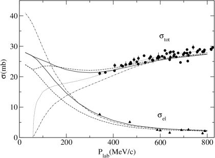
Figure 1: Total and integrated elastic $K^{+}d$ cross sections. The solid lines are the results of the full calculation. The dashed and dash-dotted lines are the results of the first-order optical potential and the single scattering impulse approximation, respectively and the dotted line is the result of Eq.(51). Phase shifts of Martinref17 are used in these calculations. The data of total cross sections are from Refs.ref8 ; ref19 ; ref20 ; ref21 ; ref22 ; ref23 ; ref24 (circles). The data of integrated elastic cross sections are from Refs.ref8 ; ref25 ; ref26 (triangles).

Now we show the calculations of the total and integrated elastic cross sections for the $K^{+}d$ scattering with the experimental data in Fig.1. The cross sections are plotted at incident momenta up to 800 MeV/c. In our calculations, the coulomb interaction is not included and the $K^{+}N$  phase shifts of Martinref17 are used.  The solid lines correspond to the full calculations including the first- and second-order optical potentials. The agreement with the data is satisfactory for both the total and elastic cross sections. For the total cross section, the theory seems to be small compared with several data at higher energies, but one can not say that there is a discrepancy between the theory and the data since the data are scattered. The dashed lines are the calculations including only the first-order optical potential. The difference between these two lines shows the size of the second-order potential effect. This effect is most important at lower energies, especially near the threshold. For the total cross section, we find that the second-order potential effect decreases its magnitude slightly at $P_{lab}\gtrapprox$ 150 MeV/c, but it increases at $P_{lab}$ $\lessapprox$ 150MeV/c. For the integrated elastic cross section, this effect increases it and such tendency becomes stronger as the energy is lower. Generally speaking, the second-order potential effect is important for the elastic cross section than the total one but it is small at $P_{lab}\gtrapprox$ 500MeV/c for both cases. The dash-dotted lines correspond to the calculations of the single scattering impulse approximation where the transition amplitude $T_{IA}$ is given as

$$T_{IA}=\left\langle\mathbf{k}^{\prime}d\left|U^{(1)}\right|\mathbf{k}d\right\rangle.$$ (50)

In this approximation, the unitarity is explicitly violated at low momenta where the elastic cross section is larger than the total cross section as shown in Fig.1. From the comparison between the dash-dotted and dashed lines, we find that the coherent rescattering effect has a significant contribution for both the total and elastic cross sections at momenta below $\sim$500 MeV/c and drastically changes the size of cross sections at low energies so as to recover the unitarity. We consider further approximation to the total cross section. We calculate it by factorizing the kaon-nucleon T matrix $t_{i}^{free}$out of integral of Eq.(43). Here the T matrix is evaluated at $\mathbf{p}_{1}=-\mathbf{k}/2$ and its form factor is taken to be $g_{l}=1$. Using the optical theorem, one gets

$$\sigma_{K^{+}d}^{tot}=K(\sigma_{K^{+}p}^{tot}+\sigma_{K^{+}n}^{tot}),$$ (51)

with

$$K =\frac{k_{0}\sqrt{s_{0}}E_{d}}{kE_{k/2}W},$$ (52)

$$k_{0}^{2} =\frac{(s_{0}-m_{K}^{2}-m^{2})^{2}-4m_{K}^{2}m^{2}}{4s_{0}},$$ (53)

where $s_{0}=(W-E_{k/2})^{2}-k^{2}/4$ and the kinematical factor $K$ approaches unity at higher energies. The dotted line is plotted using Eq.(51) and is in good agreement with the data. The difference between this line and the dash-dotted line shows the size of the Fermi motion effect which comes from the energy dependence of the kaon-nucleon amplitude. This effect decreases the magnitude of the cross section. Thus the single scattering impulse approximation underestimates the total cross section at momenta below $\sim$500 MeV/c. However, as the data of the total cross sections are rather scattered, all calculations including the full calculation are consistent with the data at momenta above $\sim$500 MeV/c.

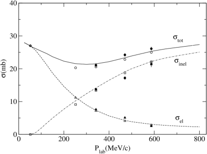
Figure 2: Total (solid line), integrated elastic (dashed line) and integrated inelastic (dash-dotted line) $K^{+}d$ cross sections given by our full calculations. The open symbols correspond to the Faddeev calculationref7 ; ref8 . The data are from Ref.ref8 ; ref27 (filled symbols). The circles, triangles and squares denote the total, integrated elasic and integrated inelastic cross sections, respectively.

In order to examine the validity of our approach, we compare our full calculation with the Faddeev calculation by Garcilazoref7 . As there are no data at momenta below 342 MeV/c, we regard the results of the Faddeev calculation as the data. We use the same kaon-nucleon T matrix used in Ref.ref7 but consider only the isospin $I=0$ S-wave nucleon-nucleon interaction as mentioned above. The results are shown in Fig.2. The solid, dashed and dash-dotted lines correspond to our full calculations for the total, integrated elastic and integrated inelastic cross sections, respectively. The integrated inelastic cross section $\sigma_{inel}$ is given by $\sigma_{inel}=\sigma_{tot}-\sigma_{el}$. The open circles, open triangles and open squares correspond to the Faddeev calculationsref7 ; ref8 for the total, integrated elastic and integrated inelastic cross sections, respectively. The open symbols at the threshold are taken from Fig.1 of Ref.ref7 . The filled symbols are the corresponding data measured by Glasser et al. ref8 ; ref27 . Our calculations are in good agreement with the Faddeev calculations as well as the data. The maximum discrepancy between our calculation and the Faddeev calculation is $6\%$ at 252MeV/c for the total cross section and $8\%$ at 587MeV/c for the elastic cross section. These results demonstrate that our model, where the optical potential contains both the first-order and second-order terms, is good enough to describe these cross sections.

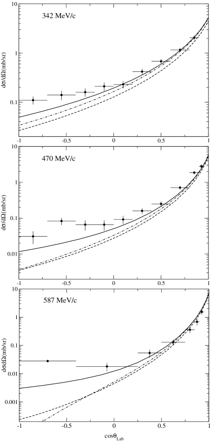
Figure 3: $K^{+}d$ elastic differential cross sections at three incident momenta. The solid line is the result of the full calculation. The dashed and dash-dotted line are the results of the first order potential and the single scattering impulse approximation. The data are from Ref.ref27 .

To see how our method predicts the elastic differential cross sections, the calculations at three incident momenta are presented with the data in Fig.3. The solid, dashed and dash-dotted lines correspond to the full calculation, the calculation with the first-order optical potential and the single scattering impulse approximation, respectively. Since the D-wave contribution in the N-N interaction is disregarded, all calculations at the backward angles are naturally underestimated. We find that the second-order optical potential makes the cross section increase and brings it close to the data at backward angles. For the forward angles, on the other hand, our full calculation is roughly consistent with the measurement as well as the Faddeev calculation shown in Figs.2-4 of Ref.ref7 .

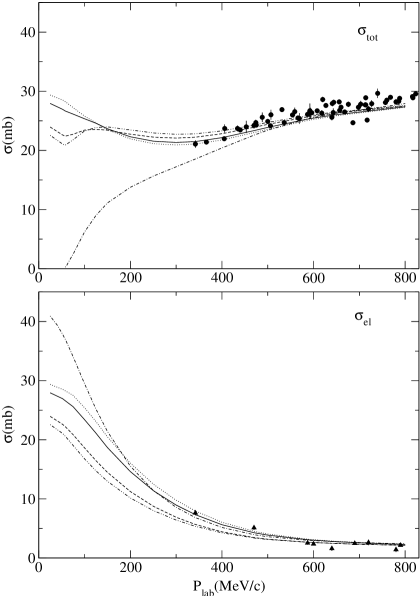
Figure 4: Total (top) and integrated elastic (bottom) $K^{+}d$ cross sections. The solid and dashed lines are the results of the full calculation and the first order optical potential, respectively. The dash-dotted line is the result of the single scattering impulse approximation. The dash-two-dotted and dotted lines are the results of the calculation with the the double scattering effect and the modified N-N scattering effect, respectively. See the details in the text. The data are the same as Fig.1.

In order to see the effects of the multiple scattering, we have calculated the total and integrated elastic cross sections using several different types of the optical potential. The results are shown in Fig.4. For reference, the calculation in the single scattering impulse approximation is plotted as dash-dotted line. The solid and dashed lines correspond to the results evaluated with $U^{\left(1\right)}+U^{\left(2\right)}$ and $U^{\left(1\right)}$, respectively. These lines are the same as Fig.1. The dash-two-dotted and dotted lines are the calculations with $U^{\left(1\right)}+U_{d}^{\left(2\right)}$ and $U^{\left(1\right)}+U_{n}^{\left(2\right)}-U_{c}^{\left(2\right)}$, respectively. The quantities $U_{d}^{\left(2\right)}$ and $U_{n}^{\left(2\right)}-U_{c}^{\left(2\right)}$ represent the effects of the double scattering and the modified N-N scattering, respectively. From the comparison of the dashed line with the dash-two-dotted line or the dotted line, we can see the size of the multiple scattering effects. Although the effects of the double scattering and the modified N-N scattering are negligible at higher momenta than 600 MeV/c, they become important with the decreasing of momentum. In the case of the total cross section shown in the top diagram of Fig.4, the double scattering term increases the cross section shown by the dashed line and the modified N-N scattering term decreases it, but at lower momenta than $\sim$100MeV/c, the effect of the two terms is completely opposite. Near the threshold, furthermore, all lines except the dash-dotted line agree with the corresponding lines in the bottom diagram of Fig.4. In the case of the elastic cross section, on the other hand, the double scattering term decreases the cross section shown by the dashed line and the modified N-N scattering term increases it. We also find that the effect of the modified N-N scattering term is larger than that of the double scattering term.

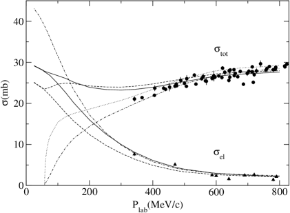
Figure 5: The same as Fig.1 except that the theoretical curves are calculated using the phase shifts of Hyslop et al.ref18 .

So far we have used the $K^{+}N$ phase shifts of Martinref17 in order to compare our calculation with the Faddeev calculation by Garcilazoref7 and check the validity of our method. Here we examine the dependence of the one-shell $K^{+}N$ amplitude. In Fig.5, we show the cross sections calculated by using the phase shifts of Hyslop et al.ref18 . At $P_{lab}>$ 500 MeV/c, the calculation is in good agreement with the data. However, at $P_{lab}\approx$ 400 MeV/c, the full calculation for the total cross section does not agree with the data. Such discrepancy can be understood from the comparison of the total cross sections given by Eq.(51) (see the dotted lines in Fig.1 and Fig.5). The total cross section represented by the dotted line in Fig.5 is slightly larger than that in Fig.1, although both of the lines almost agree with the data. Once the effects of the multiple scattering and the Fermi motion are included in the calculation, however, this tendency leads to significant difference between the two calculations of the total cross sections shown in Fig.1 and Fig.5.

IV Conclusions

The single scattering impulse approximation is able to describe the $K^{+}d$ data at incident momenta above $\sim$500 MeV/c but explicitly violates the unitarity below 200MeV/c and furthermore fails to explain the breakup reaction cross section at the forward kaon scattering angles. Accordingly the single scattering impulse approximation is not satisfactory for explaining the $K^{+}d$ scattering. Our purpose was to examine how consistently the optical potential describes the $K^{+}d$ scattering. This approach does not violate the unitarity unless an unphysical potential is used. Another advantage of the optical potential is that the calculation is straightforward compared with the Faddeev method.

We constructed the optical potential consisting of the first-order and second-order terms. The second-order optical potential includes the double scattering term and the modified N-N scattering term. The first-order and second-order potentials were evaluated without any factorization in the momentum integration. This potential was used to calculate the total, integrated elastic and elastic differential cross sections at incident momenta below 800 MeV/c. We found that our optical potential approach is able to explain both the Faddeev calculation and the data consistently and especially the second-order optical potential plays an essential role at low energies.

It was demonstrated in our calculations that the multiple scattering effects such as the coherent rescattering, the double scattering and the modified N-N scattering have an important contribution to the cross sections at low energies in spite of the weak $K^{+}N$ interaction. This importance may be related to the fact that the wave-length of $K^{+}$ is comparable to the distance between two nucleons in the deuteron. At low energies, therefore, the multiple scattering effects should be taken into account when one extracts the on-shell $K^{+}N$ amplitudes from the $K^{+}d$ data. This was confirmed through the comparison of the calculations obtained using two kinds of $K^{+}N$ phase shifts.

It is interesting to examine whether our approach is applicable for other reactions arising from the strong elementary interaction such as a $\pi d$ scattering and a $K^{-}d$ scattering. Furthermore our optical potential approach could be used to study the effect of the pentaquark resonance $\Theta(1540)$ in the $K^{+}d$ scattering and especially learn how the effects of the multiple scattering affect the suppression of the resonance peak in the $K^{+}d$ cross sections.

Our optical potential has been derived from the Watson multiple scattering theory. Similarly, the optical potential up to second order can be formulated based on the KMT multiple scattering theory as shown in Appendix. We have numerically tested the difference between two approaches. Within the first-order optical potential approach, the result by the Watson formulation does not agree with that by the KMT formulation. In the latter calculation, the integrated elastic cross section becomes larger than the total cross section at low momenta. This does not mean that the imaginary part of the KMT first-order optical potential is positive at low energies, but this is due to the factor $\frac{A-1}{A}$ appeared in the KMT formulation. When the second-order optical potential is taken into account, however, the two approaches give almost the identical cross sections. It was found from our numerical estimate that the difference was a few percent or less except near the threshold. Therefore our conclusions in this paper are not changed by which formulation is chosen.

Appendix

We will derive the optical potential from the KMT multiple scattering theory. The transition amplitude $T$ of Eq.(1) is rewritten as

$$T=\sum_{i=1}^{A}T_{i},$$ (A1)

where

$$T_{i} =\tau_{i}+\tau_{i}\frac{\mathcal{A}}{e}\sum_{j\neq i}T_{j},$$ (A2)

$$\tau_{i} =v_{i}+v_{i}\frac{\mathcal{A}}{e}\tau_{i}.$$ (A3)

In order to get the KMT optical potential $U_{KMT}$, we introduce the operator $\tilde{U}_{i}$ defined by

$$T_{i}=\tilde{U}_{i}+\tilde{U}_{i}\frac{P}{e}\sum_{j\neq i}T_{j}.$$ (A4)

In the KMT formulation, all equations are derived in the antisymmetric subspace of the Hilbert space. Consequently, the operators of $\tau_{i}$, $\tilde{U}_{i}$ and $T_{i}$ are independent of $i$. With the help of the relation $\sum_{j\neq i}T_{j}=\frac{A-1}{A}T$, Eq.(A4) can be expressed as

$$T^{{}^{\prime}}=U_{KMT}+U_{KMT}\frac{P}{e}T^{{}^{\prime}},$$ (A5)

where

$$T^{{}^{\prime}} =\frac{A-1}{A}T,$$ (A6)

$$U_{KMT} =\frac{A-1}{A}\sum_{i=1}^{A}\tilde{U}_{i}.$$ (A7)

Similarly, Eq.(A2) is written as

$$T^{{}^{\prime}}=\tau_{KMT}+\tau_{KMT}\frac{\mathcal{A}}{e}T^{{}^{\prime}},$$ (A8)

where

$$\tau_{KMT}=\frac{A-1}{A}\sum_{i=1}^{A}\tau_{i}.$$ (A9)

The scattering operator $T$ is obtained by solving Eq.(A5), if the optical potential $U_{KMT}$ is given. With the help of Eqs.(A5) and (A8),  the operator $U_{KMT}$ can be written in terms of $\tau_{i}$ as

$$U_{KMT} =\tau_{KMT}+\tau_{KMT}\frac{Q}{e}U_{KMT}$$ (A10)

$$=\frac{A-1}{A}\sum_{i=1}^{A}\tau_{i}+\frac{A-1}{A}\sum_{i=1}^{A}\tau_{i}\frac{Q}{e}U_{KMT}.$$ (A11)

Now we build the first-order and second-order optical potentials using Eq.(A11). The operator $\tau_{i}$ can be written in terms of $t_{i}$ as Eq.(10) in Sec.2. Here the operator $t_{i}$ is defined by Eq.(8). By substituting Eq.(10) into Eq.(A11), the operator $U_{KMT}$ can be expressed in terms of $t_{i}$ as

$$U_{KMT}=\frac{A-1}{A}(\sum_{i}t_{i}+\sum_{i\neq j}t_{i}\frac{1}{e}t_{j}-\sum_{i\neq j}t_{i}\frac{P}{e}t_{j}+\cdots).$$ (A12)

We note that an intermediate state in the operators $U_{KMT}$ and $t_{i}$ is either an antisymmetric state or a non-antisymmetric state. Eq.(A12) displays the KMT optical potential to second order in $t_{i}$, which corresponds to the Watson optical potential of Eq.(13). Now we consider the optical potential $U_{KMT}$ used in the calculation of the $K^{+}d$ scattering. Using the same procedure mentioned in Sec.2, we obtain the final expression

$$U_{KMT}=U_{KMT}^{(1)}+U_{KMT}^{(2)}+\cdots,$$ (A13)

with

$$U_{KMT}^{(1)} =\frac{1}{2}U^{(1)},$$ (A14)

$$U_{KMT}^{(2)} =\frac{1}{2}(U^{(2)}+\sum_{i}t_{i}^{free}\frac{P}{e}t_{i}^{free}),$$ (A15)

where the operators $U^{(1)}$, $U^{(2)}$ and $t_{i}^{free}$ are defined in Sec.2.

References

- (1) T.Nakano et al., Phys.Rev.Lett. 91, 012002(2003).
- (2) T.Nakano et al., Phys.Rev. C79, 025210(2009) and references therein.
- (3) R.N.Cahn and G.H.Trilling, Phys.Rev. D69, 011501 (2004).
- (4) W.R.Gibbs, Phys.Rev. C70, 045208(2004).
- (5) A.Sibirtsev, J.Haidenbaur, S.Krewald, and Ulf-G. Meiner, Phys.Lett. 599B,230(2004) [hep-ph/0405099].
- (6) A.Sibirtsev, J.Haidenbaur, S.Krewald, and Ulf-G. Meiner, J. Phys. G32,R395(2006) [nucl-th/0608028].
- (7) H.Garcilazo, Phys.Rev. C37, 2022(1988).
- (8) H.Garcilazo, Phys.Rev. C44, 966(1991).
- (9) K.M.Watson, Phys.Rev. 89, 575(1953).
- (10) A.K.Kerman, H.McManus, and R.M.Thaler, Ann. Phys. (N.Y.) 8, 551(1959).
- (11) R.Nagaoka and K.Ohta, Phys. Rev. C33, 1393(1986).
- (12) I.R.Afnan and A.T.Stelbovics, Phys.Rev. C23, 845(1981).
- (13) H.Garcilazo and G.Mercado, Phys.Rev. C25, 2596(1982).
- (14) M.Hirata, F.Lenz, and K.Yazaki, Ann. Phys. (N.Y.) 108, 116(1977).
- (15) D.J.Ernst, C.M.Shakin, and R.M.Thaler, Phys.Rev. C8, 46(1973).
- (16) H.Zankel, W.Plessas, and J.Haidenbauer, Phys. Rev. C28, 538(1983).
- (17) B.R.Martin, Nucl.Phys. B94, 413(1975).
- (18) J.S.Hyslop et al., Phys.Rev. D46, 961(1992).
- (19) T.Bowen et al., Phys.Rev. D2, 2599(1970).
- (20) T.Bowen et al., Phys.Rev. D7, 22(1973).
- (21) A.S.Carrol et al., Phys.Lett. 45B, 531(1973).
- (22) G.Giacomelli et al., Nucl.Phys. B37, 577(1972).
- (23) D.V.Bugg et al., Phys.Rev. 168, 1466(1968).
- (24) R.A.Krauss et al., Phys.Rev. C46, 655(1992).
- (25) G.Giacomelli et al., Nucl.Phys. B68, 285(1974).
- (26) M.Sakitt et al., Phys.Rev. D12, 3386(1975).
- (27) R.G.Glasser et al., Phys.Rev. D15, 1200(1977).