Coulomb matrix elements of bilayers of confined charge carriers with arbitrary spatial separation
Abstract
We describe a practical procedure to calculate the Coulomb matrix elements of 2D spatially separated and confined charge carriers, which are needed for detailed theoretical descriptions of important condensed matter finite systems. We derive an analytical expression, for arbitrary separations, in terms of a single infinite series and apply a u-type Levin transform in order to accelerate the resulting infinite series. This procedure has proven to be efficient and accurate. Direct consequences concerning the functional dependence of the matrix elements on the separation distance, transition amplitudes and the diagonalization of a single electron-hole pair in vertically stacked parabolic quantum dots are presented.
pacs:
71.35.Ee 0.22.60.Pn 73.21.-bThe interesting physical properties displayed by charge carriers in spatially confining settings promise to have a diverse range of applications relevant to technological developments in the near future. Systems such as semiconductor quantum wells, quantum wires and quantum dots, will have great impact in the progress of quantum computation and quantum information Nielsen and in producing new technological devices in electronics, spintronicsZutic and optoelectronics Yariv . Furthermore, on the experimental and theoretical side, systems which have acquired increasing relevance over the past decade, such as indirect excitons ButovBEC , graphene bilayers Neto and indirect magnetobiexcitons Oleg , show great promise for present-day and future understanding of condensed matter systems.
In order to grasp the full potential of these advances, it is necessary to have an increasingly detailed theoretical understanding of the physics of confined charge carriers. These studies have included, for example, learning about their optical properties, describing their response to externally applied electric fields, and understanding their behaviour when they are subject to external magnetic fields Lerner ; fqhe .
Such theoretical studies have considered, in various levels of approximation, the correlations introduced by the Coulomb interaction among charge carriers. It is well known that the physics of confined charge carriers is fundamentally affected by the Coulomb interaction between charge carriers. As a consequence, a complete theoretical study of the physical properties of charge carriers in confining settings must take into account the full and non-trivial correlations that arise from the long-ranged Coulomb interaction.
With this in sight, we present in this contribution a procedure to efficiently compute the matrix elements of the Coulomb interaction between charge carriers confined by a two dimensional parabolic potential and which are spatially separated by a general interplane distance. This particular type of physical system is relevant in the study of graphene bilayersNeto , electron bilayers Badalyan , indirect biexcitons Meyertholen , bilayer quantum Hall systems bqhe , self assembled quantum dots Kuther , coupled quantum wells Butov1999 ; Lozovik2005 , quantum dots formed by lateral fluctuations in the well Butov1994 , among many others. Having an efficient way to compute these elements opens the way for very relevant finite system calculations (i.e. particles), as opposed to the types of calculations that invoke the thermodynmic limit and that are usually encountered in some theoretical formalisms. Among the important finite system calculations, we may mention the Hartree-Fock, the Hartree-Fock-Bogoliubov (e.g. through the use of BCS-type wave functions) and the Random Phase Approximation approximations Blaizot ; Fetter .
In the case of the matrix elements of confined charge carriers moving in the same plane, the problem can be treated in an analytic form, yielding a general expression for the Coulomb matrix elements Halonen ; Jacak . However, when this formula is used for elements that involve states with high quantum numbers of either angular momenta or of radial excitations, convergence problems arise; it is then necessary to use appropriate numerical methods to obtain reliable results Boris ; Ricardo ; Alain ; Augusto . We shall see in this paper that the computation of the matrix elements for the spatially separated case also involves the use of a special numerical procedure in order to accelerate the infinite series that arises in the expansion of the expression for the Coulomb matrix elements.
This paper is organized as follows: in Sec. I, we review the Coulomb elements when the spatial separation is equal to zero. In Sec. II we give the expression for the Coulomb matrix elements calculated for the case, followed by Sec. III where the method used to accelerate convergence is explained. Finally, in Sec. IV we present some main results, and some conclusions are given in Sec. V. Appendix VI explains the notation and basis ordering used throughout the article.
I Coulomb matrix element with
The eigenfunctions of a particle subject to either a two-dimensional harmonic potential Cohen or a perpendicular magnetic field Landau are given by
| (1) |
with , , are the usual associated Laguerre polynomials and the normalization constant is given by ; all lengths are scaled by the relevant length scale of the system i.e. the harmonic oscillator length or magnetic length, a choice which depends on the external potential being considered. The corresponding energies are
| (2) |
for the harmonic oscillator basis and
| (3) |
for the Landau basis.
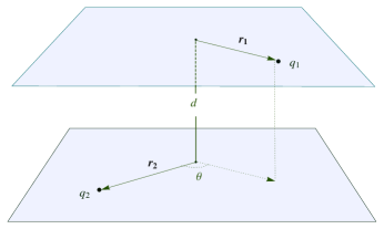
Let denote the Coulomb interaction matrix element for spatially separated charge carriers, with the length of the separation (see Fig. 1). Then, the matrix element between any two pairs of single-particle states for the case is written as
| (4) | |||||
It should be noted that is a 2D in-plane vector.
Many authors have found various expressions for these elements Halonen ; Jacak ; Tsiper . For example, using the two-dimensional Fourier transform for the Coulomb potential
| (5) |
it is possible to express the Coulomb matrix element in terms of finite sums in the form Halonen
| (6) |
The expresses the conservation of the angular momentum . We have, for convenience, defined the quantities , and .
Although expression (I) involves finite sums, it is inefficient for computing matrix elements that involve states of high angular momentum. The main difficulty arises from the computation of the large factorials. This renders the calculation of the matrix elements computationally expensive.
An alternative way of calculating the Coulomb matrix element is to write
| (7) |
By expanding the exponential inside the integral, replacing the result in (4) and integrating the angle and radial variables,we arrive at an explicit infinite series. The remaining step of calculating the infinite series was tackled successfully in BorisPhd by making use of a series acceleration algorithm (different from the one used in this work).
II The bilayer case: Coulomb matrix element with
Let us now proceed to derive an expression for the general case . The Coulomb interaction in this case reads
| (8) | |||||
being the angle between the 2D in-plane vectors and (Fig. 1), and the vector being defined as . Note that , , and are perpendicular to d. Manipulations analogous to those in the previous case, and use of lead to the following expression for the Coulomb matrix elements
where , and is the confluent hypergeometric funtion Abramowitz . This expression reduces in an equivalent form to (I) when BorisPhd . Although our expression involves an infinite sum, we can apply a numerical convergence procedure in order to make the computation of the matrix elements more tractable. To the best of our knowledge, there is no expression nor procedure for a practical calculation of the Coulomb matrix elements of spatially separated charge carriers in a two dimensional confining potential. As mentioned in the introduction, this result is of significant practical importance in finite system studies in various condensed matter systems.
Incidentally, we would like to note first that it is possible to reduce the matrix elements satisfying to only radial integrals of complete elliptic functions of the first kind , as long as . Such a simplification is not possible when mainly because of the singular behaviour of the Coulomb interaction in such a case. The resulting integrals read
| (10) |
having defined the radial function
Although the radial integrals have convergence problems for high values of the radial quantum numbers, due to the oscillatory nature of the Laguerre polynomials, the elements that can be computed agree with our results which make use of the series acceleration algorithm to be discussed presently.
III The series acceleration
We calculate the infinite series in the index that appears in (II) using a u-type Levin transform to accelerate the convergence Levin1 . The basic idea is to construct an alternate series which converges much faster than the one we have at hand. Intuitively, this could be done if there was a way to simulate the asymptotic behaviour of the remainder of the series for large values of . We can achieve this by constructing functions such that
| (12) |
being of order unity. Having done this, we can then write
| (13) |
such that the coefficients satisfy . By doing this, the asymptotic behaviour of the series will have been coded into the quantities. Now we must find a prescription for the coefficients . This can be done by writing, for large , the expression
| (14) |
This expression is reasonable so long as the functions satisfy three conditions: first, we must have and , so that (12) holds; second, for we must have when ; and third we must require that , so that, in taking the large limit, all terms vanish at the same rate. The constants are still unknown at this stage of the derivation.
With these definitions, the partial sum of our series can be written as, for large ,
| (15) |
Here, is the exact value of the series we want to compute. Finally, we truncate the sum, thus eliminating asymptotic terms:
| (16) |
The corresponding change of notation from the exact to the truncated should be clear. Notice that the expression (16) tells us that the value is such that all equations, for running from to , hold simultaneously. That is to say, the truncated value depends on all terms which add up to itself and, thus, it is as if it “feelt” the overall behaviour of the most important terms of the series. In this sense, the value calculated through the use of the u-type Levin transform can be thought of as an extrapolation of the final sum that uses information from only the first few terms of the complete series. The more terms we keep in the truncation, the better the extrapolation.
In order to find the approximation to the full sum, it is necessary to solve the equations for the unknowns and . Hence, the resulting problem of calculating the series has been reduced to computing the solution of a dimensional matrix inversion problem. The larger the value of , the better the approximation to the exact value. The u-type Levin transform uses the choices Levin1 and , which have proven to behave well for a large family of series Levin2 . The parameter is a real number that can be chosen to improve the rate of convergence.
As an example, in our calculations, an element such as
| (17) |
required terms of the series to achieve convergence up to the tenth decimal place using the term-by-term sum, whereas it required less than terms using the Levin transform, and was calculated in half the time using a standard linear solver. It should be noted that the number of terms needed to achieve convergence will depend on the matrix element that is being calculated and that the calculation time will depend on the machine and the procedure used to solve the linear system that results from the Levin transform.
IV Main results
IV.1 Comparison between the and cases
We first evaluate some particular matrix elements in order to get a feeling of how they vary as functions of the distance .
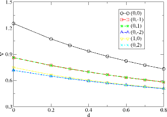
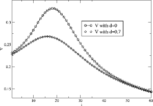
In Fig. (2), we show the behavior of the Coulomb matrix elements of the form as functions of the separation between the planes, for both the oscillator and Landau basis. For both basis sets, there is a general decaying behaviour. Clearly, when , all elements must approach zero. Refer to the appendix for the notation used for the basis sets.
Although, there is a one-to-one correspondence between both basis sets, there is a physical reason which justifies showing the calculations in both basis. The Landau basis corresponds to the solution of a charged particle moving in an external magnetic field perpendicular to the plane of motion. This system is infinitely degenerate with respect to the angular momentum quantum number and, hence, its ordering is conceptually different to the finite number of degenerate energy levels of the two dimensional harmonic oscillator system. Thus, showing the calculation in each basis set is relevant for each of the two different types of in-plane confinement.
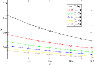
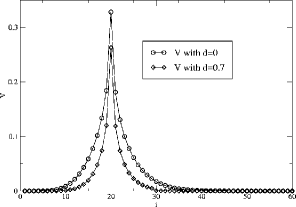
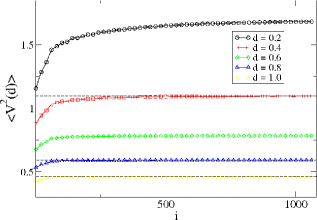
Next, we construct a set of elements which involves pairs of states with fixed total angular momentum (i.e. using sets of two-particle states with some predetermined value of their total angular momentum). In order to do this, such states were randomly chosen for the cases and . This is shown in Fig. (3). The general exponentially decaying behaviour observed in these plots seems to suggest that there is a scaling behaviour behind elements with predetermined total angular momentum.
This last observation leads to an interesting behaviour which is worth emphasizing. Although all elements get suppressed in general as the distance is increased, they do not all approach zero at the same rate. Such a behaviour can be seen clearly in the top plot of Fig.(3): one of the curves crosses two other curves, indicating that it is decaying faster than the other two. This tells us that, as varies, the entries in the matrix representation of the Coulomb interaction vary in nontrivial ways with respect to each other. In the very large limit i.e. when , we may obtain an expansion for the rate of decay
| (18) |
so that not all elements tend asymptotically to zero at the same rates, the rate depending on the indices of the states used in the matrix element. Hence it is possible, by changing the distance between the planes, for a system of charge carriers to exhibit different types of dynamical behaviour, as opposed to just interacting in a kind of screened Coulomb potential produced by the separation.
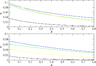
In Fig. (4) we show the most relevant elements for the dynamics of Coulombian systems, namely and , the so-called direct and exchange terms, using the first energy shell of the Landau basis. Note how, as we increase the interplane distance, the direct terms get more suppressed, relative to the value, than the exchange ones. Also, the exchange elements decay faster than the direct ones as we change the index , a behaviour that is general for every . This decay is expected because the exchange elements involve integrals of amplitudes which can interfere destructively when summed over, as opposed to the direct elements which involve probability densities which are always positive. Finally, the maximum value of the direct term is actually shifted from its diagonal value , and this maximum gets further shifted as increases. However, the maximum for the exchange plot remains at the diagonal point, although this is actually again the same diagonal (and, thus, direct) matrix element .
IV.2 Amplitude transitions and diagonaliation of a single indirect exciton
Since the Coulomb matrix elements connect two pairs of two-particle states through the Coulomb interaction, we can use them to weigh how probable it is for a particular transition to occur as a function of the distance . In order to study a simple transition, we computed the matrix elements for a given pair of initial states and several pairs of final states, all pairs having zero total angular momentum. This is shown in Fig. (5). Each continuous line is the absolute value of the transition amplitude for a given distance and each point represents a final state, as explained in the caption of the figure. The succession of lines go from through . As increases, all points (i.e. all considered transitions) generally get suppressed.
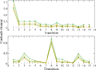
Once again, we note that the rate at which each coefficient gets suppressed is not the same for all, the diagonal transition being typically the most significant one, as further calculations of other similar cases have shown. In fact, when is of order (i.e. when the distance is of the order of the oscillator length), almost all of the coefficients are negligible, except for the diagonal ones. This reasonably shows that, when the planes are separated beyond the characteristic distance of the system, all transitions get suppressed, albeit at unequal rates.
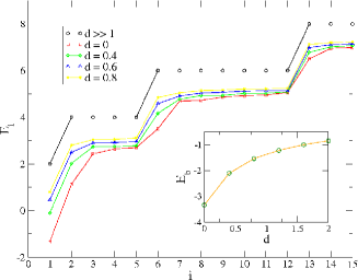
Finally, as a more physical application, we have considered the simple case of an electron and a hole spatially separated in an effective mass hamiltonian with a harmonic potential. The eigenstates of this system are those of a single spatially indirect exciton. The hamiltonian, in dimensionless units, reads
| (19) |
In this expression, we have made the convenient definition . The parameter denotes the ratio between the Coulomb and harmonic oscillator energies, and the and are the dimensionless harmonic oscillator energies of the electron and the hole, respectively. The diagonalization for the block of the hamiltonian is shown in Fig.(6). As before we notice the unequal rates of change as is varied only this time it is evidenced with the eigenenergies of the exciton. As increases, the spectrum tends to the harmonic oscillator energies for two particles with total zero angular momentum, as expected.
IV.3 Convergence sum rule
As a consistency check of the above results, we computed an identity involving the Coulomb matrix elements, reminiscent of the sum rules encountered in atomic physics. Namely, it can be checked that, provided , we can integrate out the angular integrals exactly to obtain a relation of the form
| (20) | |||
with
| (21) | |||||
Note that the convergence of the curve corresponding to is slower than that of the other curves. This has a simple and clear physical meaning. As the spatial separation between the planes becomes smaller, it will be easier for the Coulomb interaction to induce transitions starting from two particles in the oscillator ground state to two particles in two other higher oscillator states. This means that all amplitudes that we add in the sum rule become more significant as becomes smaller and, thus, the sum will require more and more terms which involve higher oscillator states. Notwithstanding this, there is clear convergence.
The radial integrals can be evaluated numerically by various methods, which makes the computation of the right hand side of (20) completely independent from our main numerical approach, which is in turn used to compute the left hand side. We found that the relation (20) was very well satisfied, as can be seen in Fig. (7).
V Conclusions
In the work presented here, we have shown the procedure and results of a numerical calculation of the Coulomb matrix elements of spatially separated charge carriers confined either by a two dimensional parabolic quantum dot or through the use of a magnetic field. We have found that, in a very important way, each matrix element is affected differently as is varied. This could lead to different and interesting physical regimes of a system subject to interparticle Coulomb interaction.
Although the procedure we have implemented above has worked quite well, it should be noted that, as with any numerical algorithm, care must be taken in evaluating elements with too high a difference in quantum numbers of the involved states e.g. high differences between the and or and . These cases can become pathological because of the highly oscillatory nature of the associated wavefunctions.
We would like to emphasize the relevance of the procedure presented here. With such elements, theoretical studies can be carried out that are comparable with experimental systems. Furthermore, this study is relevant for describing and understanding many-body effects such as collective behaviour and quantum correlations.
Work that involves the in-depth study of spatially indirect excitons
within a finite system framework using Hartre-Fock and BCS type
approximations is already on the way. For such a study, the matrix
elements computed in the present paper will be critically needed.
Acknowledgements.
The authors would like to thank the CODI - Univ. de Antioquia and the Centro de Investigaciones del ITM, for partial financial support. B.A.R. acknowledges discussions with R. Perez, A. Delgado and A. Gonzalez concerning the calculation of the case. The authors are very grateful for enlightning discussions with J. Mahecha, H. Vinck and C. Vera.VI Appendix: basis ordering
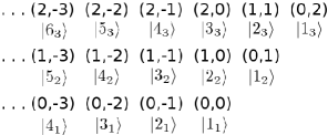
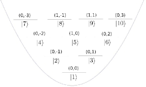
Since we will be refering to two different basis sets, we will specify the ordering used throughout the paper. Both basis sets are organized in shells according to their respective energies given in Eq.(2) and Eq.(3). For the Landau basis, the logic of the numbering can be extracted from Fig.(9); and that of the oscillator basis, from Fig.(9). The parentheses in these figures follow the notation i.e. the radial and the angular momentum quantum numbers associated to the corresponding wavefunctions shown in Eq.(1) of the charge carriers.
References
- (1) M. A. Nielsen and I. L. Chuang. Quantum Computation and Quantum Information, Cambridge University Press 2000.
- (2) I. Zutic, J. Fabian and S. Das Sarma, Rev. Mod. Phys. 76, 323 (2004)
- (3) A. Yariv and P. Yeh. Photonics: Optical Electronics in Modern Communications. Oxford University Press, 6th edition (2006).
- (4) M. Remeika, J. C. Graves, A. T. Hammack, A. D. Meyertholen, M. M. Fogler, L. V. Butov, M. Hanson, and A. C. Gossard. Phys. Rev. Lett. 102, 186803 (2009)
- (5) A.H. Castro Neto, F. Guinea, N.M.R. Peres, K.S. Novoselov and A.K. Geim. Rev. Mod. Phys. 81, 109 (2009).
- (6) O.L. Bergman, R.Y. Kezerashvili, and Y.E. Lozovik. Phys. Rev. B 78, 035135 (2008)
- (7) V. Lerner and Yu. E. Lozovik , Zh. Eksp. Teor. Fiz. 80, 1488 (1981) [Sov. Phys. JETP 53, 763 (1981)].
- (8) T. Chakraborty and P. P. Pietiläinen, The Quantum Hall Effect, Springer-Verlag, New York, (1996).
- (9) S.M.Badalyan, C.S. Kim, G. Vignale, and G. Senatore. Phys. Rev. B 75, 125321 (2007).
- (10) A.D. Meyertholen and M.M. Fogler. Phys. Rev. B 78, 235307 (2008)
- (11) M. Kellogg, J. P. Eisenstein, L. N. Pfeiffer, and K. W. West. Phys Rev. Lett 90, 246801 (2003).
- (12) A. Kuther, M. Bayer, A. Forchel, A. Gorbunov, V. B. Timofeev, F. Schafer and J. P. Reithmaier Phys. Rev. B 58, R7508 (1998).
- (13) L. V. Butov, A. A Shashkin, V. T. Dolgopolov, K. L. Campman and A. S. Gossard. Phys. Rev. B 60, 8753 (1999).
- (14) N. E. Kaputkina and Yu E. Lozovik Physica E 26, 291 (2005).
- (15) A. Zrenner, L. V. Butov, M. Hagn, G. Abstreiter, G. Böhm, and G. Weimann. Phys. Rev. Lett. 72, 3382 (1994)
- (16) J.P. Blaizot and G. Ripka Quantum Theory of Finite Systems. MIT Press, (1986).
- (17) A.L. Fetter and J.D. Walecka. Quantum Theory of Many-Particle Systems, MacGraw Hill (1971).
- (18) V. Halonen, Tapash Chakraborty and P. Pietiläinen. Phys. Rev. B 45, 5980 (1992)
- (19) Jacak L, Hawrylak P and Wojs A 1998 Quantum dots (New York: Springer-Verlag)
- (20) B. A. Rodriguez, A. Gonzalez, Phys. Rev. B 63, 205324 (2001).
- (21) R. Perez, A. Gonzalez, J. Mahecha, J. Phys.: Condens. Matter 15, 7681 (2003).
- (22) A. Delgado, A. Gonzalez, and D. J. Lockwood, Phys. Rev. B 69, 155314 (2004).
- (23) A. Gonzalez, J. D. Serna, R. Capote, and G. Avendaño, Physica E 30, 134 (2005).
- (24) Cohen-Tannoudji, C., Diu, B. and Laloë F. Quantum Mechanics. John Wiley & Sons (1977).
- (25) Landau, L. D. and E. M. Lifshitz . Quantum Mechanics: Nonrelativistic Theory. Pergamon Press (1977).
- (26) E. V. Tsiper, J. Math. Phys. 43, 1664 (2002).
- (27) B. A. Rodríguez, Núcleos artificiales. PhD Thesis, unpublished (In spanish). Universidad de Antioquia, (2002).
- (28) M. Abramowitz and I. A. Stegun, Handbook of mathematical funtions, Dover Publication, New York, (1972).
- (29) H. Homeier ArXiv:math/0005209v1 (2000).
- (30) T. Fessler and W. Ford, ACM Transactions on Mathematical Software 9 346. (1983).