Inflation on the Brane with Vanishing Gravity

Abstract:

Many existing models of brane inflation suffer from a steep irreducible gravitational potential between the branes that causes inflation to end too early. Inspired by the fact that point masses in 2+1 D exert no gravitational force, we propose a novel unwarped and non-supersymmetric setup for inflation, consisting of 3-branes in two extra dimensions compactified on a sphere. The size of the sphere is stabilized by a combination of a bulk cosmological constant and a magnetic flux. Computing the 4D effective potential between probe branes in this background, we find a non-zero contribution only from exchange of level-1 KK modes of the graviton and radion. Identifying antipodal points on the 2-sphere projects out these modes, eliminating entirely the troublesome gravitational contribution to the inflationary potential.

1 Introduction

As a solution to the horizon, flatness, heavy relic and structure formation problems in the early universe, the inflationary paradigm [1], especially in its slow-roll incarnation [2, 3], is well-established and supported by recent observations [4]. However to date there is arguably no simple and compelling canonical model in which slow-roll inflation arises generically, although there is some hope that a viable framework might be found in string theory (for reviews see [5]).

A promising example of such a framework is brane inflation [6, 7], in which the ostensibly flat brane-brane potential, in extra dimensions large compared with the brane thickness, was used for inflationary slow-roll. Large extra dimensions, with all fields except gravity confined to a brane, were originally proposed to explain the hierarchy between the weak and gravitational scales [8]. In an inflationary context they allow for sufficient separation between the branes to render gravitational effects negligibly small, with the brane tensions providing a large and constant contribution to the inter-brane potential. As the branes approach each other, the weak Newtonian gravitational attraction between them is responsible for an inflation-ending collision that could reheat the universe.

This naive expectation was called into question by Kachru et al., who argued in [9] that finite volume effects and moduli stabilization typically spoil the ‘flat’ gravitational brane potential. They concluded that viable models of brane inflation could not arise from generic string constructions with all moduli stabilized, since a correct treatment of the moduli generally renders brane potentials too steep for inflation.

The idiosyncratic nature of gravity in 2+1 dimensions has been known and understood since the 1960s: there is no Newtonian gravitational potential due to a point mass in 2+1 dimensions [10]. Instead, the mass cuts out a deficit angle from the space in which it lives, giving rise to a conical surface that is flat everywhere apart from at its location. A second point mass placed anywhere on this cone feels no gravitational force. Similarly the gravitational potential between any two codimension-2 objects in infinite flat space: for example cosmic strings in 4 dimensions, or 3-branes in 6 dimensions, is exactly constant.

Historically there has been considerable phenomenological interest in two extra spatial dimensions. In order to explain the gauge hierarchy, these naturally select millimeter-sized dimensions, which just evaded all limits from the best experimental tests of gravity at the time. The same scale also corresponded with that of the cosmological constant and neutrino masses, a coincidence that led to much model-building excitement. For example, a 2-sphere compactification of the extra dimensions, stabilized by a bulk cosmological constant and magnetic flux was used by [13, 14, 15] in order to explore the cosmological constant problem. We employ an identical configuration as a background in which to explore brane inflation [16], seeking a general unwarped mechanism to flatten the steep irreducible gravitational contribution to the inter-brane potential. Unlike previous analyses which contain exact solutions in the presence of finite-tension branes in specific configurations, we treat the branes as purely gravitational perturbations at arbitrary positions on the stabilized 2-sphere. We then compute the solution to leading order in this perturbation by integrating out all interacting massive KK modes in the 4D effective theory.

We begin this paper with a careful analysis of Kachru et al.’s assertion that extra dimensional brane inflation does not generically work (see Section 2). We couch their argument in terms of a shape function for the inflaton potential, which makes it evident that the inflationary parameter $\eta$ is independent of all dimensionful parameters. We then explain, from the perspective of the 4D effective theory, the need for a volume subtraction in closed spaces. This constrains $\eta$ to be an $\mathcal{O}(1)$ quantity, which is too large for successful slow-roll inflation. In Section 3.1 we attempt to understand perturbatively the behavior of point masses in 2+1 D. We subsequently examine two 3-branes in a flat 6D space in Section 3.2, and find that the potential due to graviton exchange is exactly zero as expected. From the standpoint of the 4D effective theory, we find that this lack of gravitational potential results from a direct cancellation between the potential due to the exchange of massive graviton and radion modes. We show in Section 3.3 that this is no longer the case in a spherical background stabilized by a bulk cosmological constant and magnetic flux. Rather, the potential only vanishes for $\ell\geq 2$ spherical harmonic modes; exchange of the $\ell=1$ modes gives rise to a repulsive cosine potential that is again too steep, ending slow-roll inflation early. This striking outcome suggests a simple solution: identifying antipodal points on the 2-sphere projects out odd KK modes, again giving exactly zero potential between the branes. We discuss two possibilities for adding an interaction that would make this setup the basis for a viable model of inflation: a massive bulk scalar coupling to the branes, and the effect of the gravitational casimir between branes. Finally we discuss the effect of dialing up the brane tensions so they can no longer be treated as perturbations on the spherical background, but instead cut out finite deficit angles from the extra dimensional space. We predict zero gravitational potential even in this limit, and make some observations about existing models with codimension-2 branes.

Throughout this paper we use the field theorist’s mostly minus metric sign convention $(+-----)$, with uppercase Roman letters labelling 6D coordinates $X^{M}$ with metric $g_{MN}$; lowercase Greek for extended 4D Minkowski coordinates $x^{\mu}$ with metric $g_{\mu\nu}$; and lowercase Roman for coordinates in the extra dimensions $y^{m}$ with metric $g_{mn}$.

2 Pitfalls of Brane Inflation

The original brane inflation scheme [6] treated branes as point particles in infinite flat extra dimensions. Naively the potential due to two branes, a distance $r$ apart, can be thought of as the sum of their brane tensions ($f^{4}$) and the Newtonian potential between them in $n$ extra dimensions:

$$V(r)=f_{1}^{4}+f_{2}^{4}+\frac{1}{M^{D-2}}\frac{f_{1}^{4}f_{2}^{4}}{r^{n-2}}$$ (1)

where $D$ is the total number of dimensions and $M$ is the fundamental Planck scale. This potential looks remarkably flat when the branes are far from each other since the tension terms dominate over the negligible gravitational potential (see Fig. 1).

\psfrag{Vr}{$V(r)$}\psfrag{BraneSize}{$\frac{1}{f}$}\psfrag{r}{$r$}\includegraphics[width=325.215pt]{braneinf}

Figure 1: The Newtonian potential between branes in infinite flat extra dimensions is nearly constant when the branes are far apart by comparison with their size ($1/f$), since the gravitational attraction between them is negligible.

For a large enough extra dimension compared with the size of the branes ($1/f$), it seems like it should be possible for the branes to get far enough away from each other to sample the flat region of the potential. However there are two problems with this naive argument. First, the slow roll parameter $\eta$ also involves the 4D Planck mass; we will show below that this results in a cancellation between all the dimensionful parameters in the theory, leaving $\eta$ dependent on a single dimensionless function of the angular separation of the branes. Because of this, hierarchies between dimensionful parameters cannot affect $\eta$. Moreover, the Newtonian potential in Eq. (1) needs to be modified for a compact space; we show why this is, and how it prevents $\eta$ from being small enough for a successful theory of slow-roll inflation.

Factoring out dimensionful quantities from the potential between two branes of equal tension $f^{4}$:

$$V(\theta)=2f^{4}+\frac{1}{M^{D-2}}\ \frac{f^{8}}{L^{n-2}}\ \varphi(\theta)$$ (2)

where $L$ is the size of the space and $\varphi(\theta)$ is a dimensionless function describing the shape of the potential.

As argued in [17], the Lagrangian for two branes labeled by $i$ at positions $\vec{Y}_{i}$, is given by the measure on each brane,

$$\mathcal{L}\ =\ \sum f^{4}_{i}\sqrt{g_{\mu\nu}(\vec{Y}_{i})}\ \simeq\ f^{4}\,\left(\partial_{\mu}\Delta\vec{Y}\right)\cdot\left(\partial^{\mu}\Delta\vec{Y}\right)$$ (3)

then the inflaton field $\Phi$ is the canonically normalized distance between the branes, $|\Delta\vec{Y}|$

$$\Phi^{2}=f^{4}\,\Delta\vec{Y}^{2}=f^{4}\,L^{2}\,\theta^{2}$$ (4)

The inflationary parameter $\eta$ is defined in terms of the Hubble constant $H$ as follows:

$$\eta \equiv \frac{m_{\Phi}^{2}}{H}=M_{4}^{2}\frac{V^{\prime\prime}(\Phi)}{V(\Phi)}$$ (5)

$$\simeq \varphi^{\prime\prime}(\theta)\qquad\textrm{for large brane separation}$$

where $M_{4}$ is the 4D Planck mass, $M_{4}^{2}=M^{D-2}L^{n}$. As claimed, $\eta$ is independent of all dimensionful quantities, and depends only on the shape of a dimensionless potential.

The Newtonian potential at position $\vec{y}$ in $n$ extra dimensions, due to a brane with tension $f^{4}$ at the origin, is governed by the Poisson equation:

$$\nabla^{2}\phi(\vec{y})=\frac{f^{4}}{M^{D-2}}\delta^{(n)}(\vec{y})$$ (6)

This equation is inconsistent for a closed space since the left side is a total derivative and so integrates to zero. Kachru et al. modify this by subtracting a volume-dependent term that “emerges naturally from the curvature of the four-dimensional space-time” [9].

$$\nabla^{2}\phi(\vec{y})=\frac{f^{4}}{M^{D-2}}\left(\delta^{(n)}(\vec{y})-\frac{1}{L^{n}}\right)$$ (7)

We argue that this correction actually emerges from a careful treatment of the zero mode in the 4D effective theory, even in a flat, closed space.

Recall that the low-energy effective potential between two branes can be computed by integrating out all the heavy KK modes coupling to them. Zero modes coupling to the branes however, should be treated differently: they must remain in the effective theory, and will in general give rise to a time-dependent cosmological expansion. Hence the Green’s function for the potential in a compact space must include a sum over all modes except for the zero mode. We illustrate this point below using the example of the potential due to point masses on an $n$-torus, and show that the seemingly ad hoc volume subtraction corresponds exactly to leaving out the zero mode from the sum over modes in the Green’s function.

To solve for the potential due to a point mass $m$ on an $n$-torus of radius $L$, we first transform the naive flat-space Poisson equation, Eq. (6), into momentum space to obtain

$$\vec{k}^{2}\tilde{\phi}_{\vec{n}}=\frac{m}{M^{n+2}}e^{-i\vec{k}_{n}.\vec{y}}\qquad\qquad{\rm with}\qquad\qquad\vec{k}_{n}=\frac{2\pi\vec{n}}{L}$$ (8)

for each fourier mode $\tilde{\phi}_{\vec{n}}$. This equation is obviously inconsistent for $\vec{n}=0$ and should be modified by subtracting off the zero mode contribution from the right-hand-side.

$$\vec{k}^{2}\tilde{\phi}_{\vec{n}}=\frac{m}{M_{4}^{2}}\left(e^{-i\vec{k}_{n}\vec{y}}-\delta_{\vec{n},0}\right)$$ (9)

This corresponds to not integrating the zero mode out of the effective theory and leaving $\tilde{\phi_{0}}$ unconstrained. The corrected equation is exactly the fourier transform of the modified Poisson equation, Eq. (7), with the $\vec{y}$-independent volume term corresponding to a Kronecker delta which picks out the zero mode, thus justifying the volume subtraction.

We now factorize out all dimensionful quantities as before to obtain the following equation for the dimensionless potential $\varphi$,

$$\nabla^{2}\varphi(\vec{\theta})=\left(\delta^{(n)}(\vec{\theta})-1\right)$$ (10)

which, away from all sources, is simply

$$\left(\partial_{1}^{2}+\cdots+\partial_{n}^{2}\right)\varphi(\vec{\theta})=-1$$

This sum of second derivatives, which determines the slow roll parameter $\eta$, will be minimized if we distribute it evenly in all directions, giving $|\varphi^{\prime\prime}(\theta)|>1/n$. This constraint is a direct consequence of the modification in Eq. (7), and results in a hard lower limit for $\eta$ that depends on the number of branes and the number of extra dimensions, both of which are $\mathcal{O}(1)$ quantities.

3 Vanishing Gravity in Codimension 2

The non-Newtonian nature of 2+1 D gravity provides a simple and elegant way around these issues. Point masses in infinite, flat codimension 2 do not attract each other, but simply cut out deficit angles that are proportional to their masses, giving rise to conical spaces that are flat everywhere apart from at the location of the masses [10]. For completeness we review the argument for this below.

3.1 Static point masses in 2+1 dimensions

We use the following ansatz for the line element (recall that 2 spatial dimensions are conformal to flat space):

$$ds^{2}=dt^{2}-\omega(x,y)\left(dx^{2}+dy^{2}\right)$$

For a single point mass at the origin of the space, the only non-trivial component of Einstein’s equation is:

$$-\frac{1}{2}\nabla^{2}\ln{\omega}=\frac{m}{M}\delta(\vec{r})$$ (11)

where $\nabla^{2}$ is the flat Laplacian, $m$ is the mass of the source, and $M$ is the 2+1 D fundamental scale. We solve this to obtain

$$\omega=\left|\vec{r}\right|^{-\frac{m}{\pi M}}$$

Going to polar coordinates in the spatial dimensions gives a metric:

$$ds^{2}=dt^{2}-r^{-\frac{m}{\pi M}}\left(dr^{2}+r^{2}d\theta^{2}\right)$$

but by making the coordinate redefinitions

$$\rho=\frac{1}{1-\frac{m}{2\pi M}}r^{1-\frac{m}{2\pi M}}\;;\qquad\theta^{\prime}=\left(1-\frac{m}{2\pi M}\right)\theta$$

we see that it indeed looks flat, with an additional restriction on the polar angle:

$$ds^{2}=dt^{2}-d\rho^{2}-\rho^{2}d\theta^{\prime 2}\qquad\textrm{where}\qquad 0\leq\theta^{\prime}\leq 2\pi-\frac{m}{M}$$

This is the metric for a circle with deficit angle $\delta=m/M$ cut out, and the two boundaries of the deficit identified, forming a cone with the point mass at its apex (see Fig. 2). The static solution for multiple point masses is a space where each one cuts out a deficit angle that is proportional to its mass, with no gravitational force between them.

\psfrag{m}{$m$}\psfrag{delta}{\!\!\!$\delta=\frac{m}{M}$}\psfrag{m1}{$m_{1}$}\psfrag{m2}{$m_{2}$}\psfrag{delta1}{\!\!\!\!\!$\delta_{1}=\frac{m_{1}}{M}$}\psfrag{delta2}{\!\!$\delta_{2}=\frac{m_{2}}{M}$}\includegraphics[height=86.72377pt]{pie}

\psfrag{m}{$m$}\psfrag{delta}{\!\!\!$\delta=\frac{m}{M}$}\psfrag{m1}{$m_{1}$}\psfrag{m2}{$m_{2}$}\psfrag{delta1}{\!\!\!\!\!$\delta_{1}=\frac{m_{1}}{M}$}\psfrag{delta2}{\!\!$\delta_{2}=\frac{m_{2}}{M}$}\includegraphics[width=28.90755pt]{right_arrow}

\psfrag{m}{$m$}\psfrag{delta}{\!\!\!$\delta=\frac{m}{M}$}\psfrag{m1}{$m_{1}$}\psfrag{m2}{$m_{2}$}\psfrag{delta1}{\!\!\!\!\!$\delta_{1}=\frac{m_{1}}{M}$}\psfrag{delta2}{\!\!$\delta_{2}=\frac{m_{2}}{M}$}\includegraphics[height=86.72377pt]{cone}

\psfrag{m}{$m$}\psfrag{delta}{\!\!\!$\delta=\frac{m}{M}$}\psfrag{m1}{$m_{1}$}\psfrag{m2}{$m_{2}$}\psfrag{delta1}{\!\!\!\!\!$\delta_{1}=\frac{m_{1}}{M}$}\psfrag{delta2}{\!\!$\delta_{2}=\frac{m_{2}}{M}$}\includegraphics[height=86.72377pt]{tent_pie}

Figure 2: A point mass in 2+1 dimensions cuts out a deficit angle $\delta$ proportional to its mass (left), with the two boundaries of the deficit identified, forming a cone with the mass at its apex (center). Multiple point masses each cut out their own deficit angles, yielding as a static solution a space that is flat everywhere except at the positions of the sources (right). Each mass has no effect on any other - there is no gravitational force between them.

Since it similarly satisfies Eq. (11) in the extra dimensions, a 3-brane in a 6-dimensional space also cuts out a deficit angle proportional to its tension. There is thus no gravitational attraction between codimension-2 branes, circumventing altogether the issue of a steep irreducible gravitational potential.

We explore this idea in detail below, studying the full 6D problem in the perturbative limit, to leading order in the brane sources. Our initial goal is to understand the vanishing gravitational potential from the perspective of the 4D effective theory. We then use this knowledge to seek a realistic inflationary model where the 2 extra dimensions are compactified and stabilized.

3.2 Perturbative codimension 2: flat space

We compute the effective potential by integrating out the 6D graviton in the Einstein-Hilbert Lagrangian with a brane source term (setting the 6D fundamental scale M=1 for simplicity)

$$\mathcal{L}=-\sqrt{\left|g\right|}\left(\frac{1}{2}R+\frac{1}{2}T_{MN}H^{MN}\right)$$ (12)

where $T_{MN}$ is the energy-momentum tensor for a brane with tension $f^{4}$ at position $\vec{y}=\vec{y}\,^{\prime}$. This is only non-zero along the brane:

$$T_{MN}=\left\{\begin{array}[]{cr}f^{4}\,\delta\left(\vec{y}-\vec{y}\,^{\prime}\right)\eta_{\mu\nu}&\ \ {\rm for\ \ M,N=0,\cdots,3}\\ 0&{\rm otherwise}\end{array}\right.\ \ \ .$$ (13)

The potential between two brane sources is

$$V=T^{(1)}_{MN}P^{MN\,OP}T^{(2)}_{OP}$$ (14)

with the graviton propagator $P^{MN\,OP}$ computed by inverting the quadratic part of the gauge-fixed Lagrangian. In de Donder gauge, the propagator in $D$ flat space-time dimensions is

$$P^{MN\,OP}=\frac{1}{k^{2}}\left(\tfrac{1}{2}\,\eta^{MO}\eta^{NP}+\tfrac{1}{2}\,\eta^{MP}\eta^{NO}-\tfrac{1}{D-2}\,\eta^{MN}\eta^{OP}\right)$$ (15)

For a $(d\!-\!1)$-brane this yields a potential:

$$V \sim \eta_{\mu\nu}\left(\tfrac{1}{2}\,\eta^{JM}\eta^{KN}+\tfrac{1}{2}\,\eta^{JN}\eta^{KM}-\tfrac{1}{D-2}\,\eta^{JK}\eta^{MN}\right)\eta_{\sigma\rho}$$

$$= \frac{1}{2}d+\frac{1}{2}d-\frac{d^{2}}{D-2}$$

$$= 0\qquad\textrm{for }D=d+2\qquad\textrm{(codimension 2)}$$

By compactifying this space on a flat 2-torus one can understand the mechanism by which this cancellation occurs in the 4D effective theory. We sketch below the argument showing that it stems from a mode-by-mode cancellation between Kaluza-Klein (KK) modes of the 4D graviton tower and those of the 4D radion tower.

The 6D metric perturbation $H_{MN}$ around a flat background can be parametrized as follows:

$$H_{MN}=\left({\begin{array}[]{*{20}c}{h_{\mu\nu}-2\Phi\eta_{\mu\nu}}&{V_{\mu n}}\\ {V_{\nu m}}&{\phi_{(mn)}+2\Phi\eta_{mn}}\\ \end{array}}\right)$$ (17)

where parentheses indicate trace-subtracted indices, e.g. $\eta_{mn}\phi^{(mn)}=0$.

Not all these are physical degrees of freedom since there are gauge redundancies: specifically 6 general coordinate transformation degrees of freedom which need to be fixed. In this simple scenario it is easy to choose a gauge that decouples all fields at quadratic order:

$$\partial^{m}V_{\mu m}=0\qquad\qquad\partial\phi_{(mn)}+4\partial_{n}\Phi=0$$ (18)

Canonically normalizing the independent physical fields, we encounter a tower of graviton and radion KK modes of equal mass $m_{(i,j)}$, with propagators $P_{(i,j)}^{\mu\nu\,\rho\sigma}$ and $P_{(i,j)}$ respectively. We can now compute the contribution to the potential between branes in the limit of conserved sources, due to integrating out the graviton and radion towers. For each mode $(i,j)$ we find a potential

$$V_{\left(i,j\right)} \sim \left(\eta_{\mu\nu}P_{(i,j)}^{\mu\nu\sigma\rho}\eta_{\sigma\rho}+\frac{2}{\sqrt{3}}P_{(i,j)}\frac{2}{\sqrt{3}}\right)$$

$$\propto -\frac{4}{3}+\frac{4}{3}=0$$

i.e. at each level the radion KK mode provides an attractive force that is exactly equal to the repulsive force due to the graviton KK mode: mode by mode the force cancels.

With no gravitational attraction between them, 3-branes in infinite 6D are stable. However, they source a linear potential for the (zero mode) radion in the effective theory, which sets the size of the compact space, causing it to run away to infinity. A reliable, calculable theory of brane inflation must provide a mechanism to stabilize all zero modes that couple to the inflaton field [9].

The first example of a successful stabilization method for compact extra dimensions was due to Freund and Rubin [18], who employed a combination of a bulk cosmological constant and an extra-dimensional magnetic flux to give a mass to the radion mode, fixing the radius of the $n$-sphere. We use this mechanism to stabilize 2 extra dimensions compactified on a sphere [19], and compute the 4D effective potential between static probe branes in this $\rm{Minkowski}_{4}\times S_{2}$ background (see Fig. 3).

\psfrag{Fmn}{\;\;$F_{mn}$}\psfrag{L6}{$\Lambda$}\psfrag{B}{$B$}\includegraphics[height=93.95122pt]{sphere_flux}

\psfrag{Fmn}{\;\;$F_{mn}$}\psfrag{L6}{$\Lambda$}\psfrag{B}{$B$}\includegraphics[height=93.95122pt]{sphere_with_branes}

Figure 3: Compact 2-sphere stabilized by combination of 6D cosmological constant and extra-dimensional magnetic flux (left); two probe-branes on stable 2-sphere (right).

3.3 Perturbative codimension 2: compact 2-sphere

The compactified background metric takes the form of a 2-sphere orthogonal to infinite 4D Minkowski space:

$$ds^{2}=\eta_{\mu\nu}dx^{\mu}dx^{\nu}-r^{2}\left(d\theta+\sin^{2}\theta\ d\phi\right)$$

In addition to the Einstein-Hilbert term, the stabilized Lagrangian contains a 6D cosmological constant and an electromagnetic field strength tensor:

$$\mathcal{L}=-\sqrt{\left|g\right|}\left(\frac{1}{2}R+\Lambda+\frac{1}{4}F_{MN}F^{MN}\right)$$ (20)

Expanding this to linear order in perturbations $H_{MN}$ about the background metric $\overline{g}_{MN}$, gives Einstein’s equation for the background:

$$\left(\overline{R}_{MN}-\frac{1}{2}\overline{g}_{MN}\overline{R}\right)=\overline{g}_{MN}\Lambda+\frac{1}{4}\overline{g}_{MN}\overline{F}_{OP}\overline{F}^{OP}-\overline{F}_{MO}\overline{F}_{N}^{\ O}$$ (21)

In general the background electromagnetic field strength must also be perturbed in order to obtain a consistent solution for Einstein’s equation with arbitrary sources. We confirm in Appendix A that the total flux through the sphere is unaffected by the presence of such a perturbation, which is defined as follows:

$$F_{MN}=\overline{F}_{MN}+f_{MN}$$

and can be written in terms of a dimensionless gauge potential $b_{N}$, and a constant, $B$:

$$B\,f_{MN}=\nabla_{M}b_{N}-\nabla_{N}b_{M}=\overline{\nabla}_{M}b_{N}-\overline{\nabla}_{N}b_{M}$$

Setting the linear coefficient of $b_{N}$ in the Lagrangian to zero gives Maxwell’s equation $\overline{\nabla}_{M}\overline{F}^{MN}=0$, one possible solution to which is non-zero only in the extra-dimensional magnetic components:

$$\bar{F}_{MN}=\left\{\begin{array}[]{cr}0&\ \ {\rm for\ M,N=0,\cdots,3}\\ B\,\epsilon_{mn}&\ \ {\rm otherwise}\end{array}\right.$$ (22)

where $\epsilon_{mn}$, the extra-dimensional spherical surface-area element, is related to the totally antisymmetric tensor $\varepsilon_{mn}$ by $\epsilon_{mn}=\sqrt{g_{mn}}\varepsilon_{mn}$ (with $\varepsilon_{45}=1$). The constant $B$ is now seen to be the strength of the magnetic field.

The 6D and 4D trace of Einstein’s equations relate the magnetic field $B$ and cosmological constant $\Lambda$ to the radius of the sphere $r$:

$$\Lambda=\frac{1}{4}\overline{F}_{mn}\overline{F}^{mn}=\frac{1}{2}B^{2}=-\frac{1}{4}\overline{R}=\frac{1}{2r^{2}}$$ (23)

where $\overline{R}$ is the background Ricci scalar. This fixes all components of the Riemann Tensor in this background,

$$\overline{R}_{MNOP}=-\overline{F}_{MN}\overline{F}_{OP}\\$$ (24)

and sets to zero the sum of the constant background terms in the Lagrangian (20), as expected for an effective 4D Minkowski space.

Including a source term for the branes, which have energy-momentum tensor $T_{MN}$ given by Eq. (13), and simplifying using the background solution (Eqs. (21) and (24)), the Lagrangian to quadratic order in perturbations is:

$$\mathcal{L} = \frac{1}{4}H^{MN}\left[\frac{1}{2}\left(g_{MN}g_{OP}-g_{MO}g_{NP}\right)\nabla^{2}+g_{NP}\left(\nabla_{M}\nabla_{O}+R_{MO}\right)-g_{MN}\nabla_{O}\nabla_{P}\right]H^{OP}$$ (25)

$$+ \frac{1}{4}H^{MN}\left[4F_{MO}f_{N}^{\ O}-g_{MN}F_{OP}f^{OP}\right]-\frac{1}{4}f_{MN}f^{MN}-\frac{1}{2}H^{MN}T_{MN}$$

where we have omitted the bars denoting background quantities for simplicity. This Lagrangian yields the following linear equations of motion for $H^{MN}$ and $b^{N}$:

$$g_{MN}\big{(}\nabla^{2}\!H-\nabla_{O}\!\nabla_{P}H^{OP}\!\!-F_{MN}f^{MN}\big{)}-\nabla_{M}\!\nabla_{N}H-\nabla^{2}\!H_{MN}\hskip 86.72377pt$$ (26)

$$+\Big{[}\left(\nabla_{M}\!\nabla_{O}+R_{MO}\right)\!H_{N}^{\ O}+2F_{MO}f_{N}^{\ O}\!+\left(m\!\!\leftrightarrow\!n\right)\Big{]} = 2\;T_{MN}$$

$$-\frac{1}{2}F^{MN}\nabla_{M}H+\nabla_{M}H_{O}^{\ M}F^{ON}-\nabla_{M}H_{O}^{\ N}F^{OM}-\nabla_{M}\nabla^{M}b^{N}+\nabla_{M}\nabla^{N}b^{M} = 0\ \ .$$

We KK reduce by parameterizing the metric perturbations as follows:

$$H_{MN}=\left({\begin{array}[]{*{20}c}{h_{(\mu\nu)}+2\Psi\eta_{\mu\nu}}&{V_{\mu n}}\\ {V_{\nu m}}&{\phi_{(mn)}+2\Phi g_{mn}}\\ \end{array}}\right)$$ (27)

Note that we separate the 4D component into traceless part and trace part and do not make a Weyl transformation, for reasons that will become clear later. The gauge field perturbation $b_{M}$ is decomposed as

$$b_{M}=\left({\begin{array}[]{*{10}c}b_{\mu}\\ \epsilon_{km}\nabla^{k}b+\nabla_{m}b^{\prime}\\ \end{array}}\right)$$ (30)

Due to the non-zero curvature and magnetic flux, there is no viable gauge in which all the physical fields in this particular parametrization are decoupled. We gauge fix as follows, making sure to also fix the additional $U(1)$ gauge freedom:

$$\nabla_{n}V^{n\mu}=0\qquad\qquad\nabla_{n}\phi^{(mn)}=0\qquad\qquad\nabla_{n}b^{n}=0$$ (31)

which sets to zero the following:

$$\phi^{(mn)}=0\qquad\qquad b^{\prime}=0.$$ (32)

We can parametrize the extra-dimensional dependence of the 4D scalar fields using scalar spherical harmonics $Y_{\ell,m}(\theta,\phi)$. Then we can perform a separation of variables as follows:

$$\nabla_{M}\nabla^{M}\psi\left(x^{\mu},\theta,\phi\right)=\left(\Box+\triangle\right)\psi\left(x^{\mu}\right)Y\left(\theta,\phi\right)$$ (33)

for a general field $\psi$, where $\Box=\partial_{\mu}\partial^{\mu}$, and $\triangle Y=\nabla_{m}\nabla^{m}Y=r^{-2}\ell\left(\ell+1\right)$.

We compute the potential by integrating out the massive scalar KK modes for static brane sources ($p_{\mu}p^{\mu}\ll m^{2}$) by inverting the scalar mass matrix. The quadratic mass mixing at each KK level in the Lagrangian (suppressing all spherical harmonic $\left(\ell,m\right)$ indices for simplicity) takes the form

$$\mathcal{L}\supset r^{-2}\ell(\ell+1)\left(\Psi\quad\Phi\quad b\right)\cdot\left(\begin{array}[]{ccc}6&2&-2\\ 2&-\frac{2}{\ell(\ell+1)}&1\\ -2&1&-\frac{\ell(\ell+1)}{2}\\ \end{array}\right)\cdot\left(\begin{array}[]{c}\Psi\\ \Phi\\ b\\ \end{array}\right)$$ (34)

For $\ell\geq 2$ this mass matrix is invertible, giving rise to a potential

$$V\sim\left(\begin{array}[]{ccc}1&0&0\end{array}\right)\cdot\left(\begin{array}[]{ccc}6&2&-2\\ 2&-\frac{2}{\ell(\ell+1)}&1\\ -2&1&-\frac{\ell(\ell+1)}{2}\\ \end{array}\right)^{-1}\cdot\left(\begin{array}[]{c}1\\ 0\\ 0\end{array}\right)=0\ \ .$$ (35)

For $\ell\!=\!1$ however, the mass matrix has a zero eigenvalue. This is not due to the presence of a physical massless field, but rather due to an additional gauge redundancy, corresponding to conformal diffeomorphisms on the sphere [20, 21], which needs to be fixed. The static quadratic Lagrangian for $\ell=1$ is only a function of $\Psi$ and the combination $\chi=\Phi-b$, and is completely independent of the orthogonal combination $\chi_{\perp}=\Phi+b$, which is a pure gauge mode and drops out. The mass matrix in the $\{\Psi,\chi\}$ basis can be inverted to yield a potential between two branes of equal tension $f^{4}$, separated by angle $\theta$ on the sphere, of

$$V=\frac{2f^{8}}{5M^{4}}\sum_{m=-1}^{+1}\overline{Y_{1m}}(0,0)Y_{1m}(\theta,\phi)=\frac{3f^{8}}{10\pi M^{4}}\cos(\theta)$$ (36)

This repulsive potential between the probe branes gives a dimensionless shape function $\varphi\left(\theta\right)$ that goes like $\cos\left(\theta\right)$. Hence $\eta\sim-\cos\left(\theta\right)$ which is $O\left(1\right)$ for arbitrary positions of the branes on the sphere. Furthermore, although $\eta(\pi/2)=0$, the force between the branes is maximal and repulsive, at this point, yielding an unstable configuration. These results are confirmed by analyzing the linearized equations of motion for the KK modes in Appendix B.

We want to emphasize that, from the perspective of the 4D effective theory, the simplicity of this result is rather surprising. We saw above that the absence of a gravitational potential between two codimension-2 sources in a flat background could be perturbatively attributed to a mode-by-mode cancelation between the graviton KK tower and the radion KK. One might expect that stabilizing the space by giving a mass to the radion mode while keeping the graviton massless would shift the masses of the entire radion KK tower while leaving the graviton tower untouched, spoiling the cancelation at every KK level. This also what one would naively expect from examining the quadratic Lagrangian, Eq. (25): the background curvature $R_{MO}$, having only extra-dimensional components, acts like an extra contribution to the mass of the radion tower, and has no effect on the graviton tower. However, mixing with the flux perturbation can be thought of as undoing this effect for $\ell\geq 2$, leaving only the contribution from the $\ell=1$ mode for arbitrary brane positions. The exact mechanism by which this cancellation takes place can be elucidated only by diagonalizing the full quadratic Lagrangian, including kinetic terms, in order to identify the real propagating degrees of freedom. Details can be found in a follow-up paper [22].

The striking simplicity of the resulting potential allows for a similarly simple solution: a spherical background that has antipodal points identified is also a solution to the background equations, but one with all odd KK modes projected out, excluding the problematic $\ell=1$ mode from the spectrum. This space can be thought of as the real projective space $P_{2}$ (see Fig. 4, left panel), or equivalently as the entire $S_{2}$ with brane sources appearing in antipodal pairs (Fig. 4, right panel).

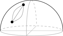
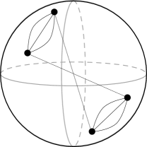
Figure 4: A single brane on the projective space $P_{2}$ (left) can be equivalently thought of as an antipodal pair of branes on $S_{2}$ (right). This setup projects out all odd KK modes, setting to zero the gravitational potential for arbitrary brane positions.

It is evident from considering the lower-dimensional effective theory that the brane tension here plays the role of the 4D vacuum energy: taking the tension to zero results in a static space that does not inflate. This relationship between the brane tension and the 4D cosmological constant is quantified, in the non-perturbative limit with finite-tension branes, in Appendix C. It is natural to ask whether our result of zero gravitational potential still applies in this limit. The following intuitive argument suggests that it does. Dialing up the brane tension, in the antipodal-pair picture each pair of branes cuts out a slice of the sphere of angular size proportional to its tension. These slices can be chosen to have no overlap with each other, in which case it is clear that the first pair of branes has no effect on the second pair, and the gravitational potential is zero (see Fig. 5). In addition, the fact that the potential before the projection was repulsive ensures the stability of any finite-tension setup with maximally separated branes, e.g. the football configuration in [14].

Figure 5: Two antipodal pairs of branes with finite tension each cut out their own deficit angle. These regions can be chosen not to overlap, implying zero (gravitational) interaction.

One might still be concerned about the stability of our setup being jeopardized by the presence of three further massless modes, corresponding to orthogonal fluctuations of the branes in the extra dimensions. However these are ‘eaten’ by an $SU(2)$s-worth of gauge bosons (originating in the off-diagonal elements of the 6D graviton) [25, 26], which then get a mass $m_{SU(2)}\sim\sqrt{\delta}/r$.

\psfrag{E}{$E$}\psfrag{M4}{$M_{4}$}\psfrag{M}{$M=\sqrt{\frac{M_{4}}{r}}$}\psfrag{Lambda6}{$\sqrt[6]{\Lambda_{6D}}\sim\sqrt[3]{B}\sim\sqrt[3]{\frac{M_{4}}{r}}$}\psfrag{f}{$f=\sqrt[4]{\delta}M\sim\sqrt[4]{\Lambda_{4D}}$}\psfrag{size}{$\frac{1}{r}$}\psfrag{H}{$H\sim m_{SU(2)}\sim\frac{\sqrt{\delta}}{r}$}\includegraphics[width=50.58878pt]{scales}

The different scales in this construction and their relationship to each other can be seen on the left. Note that the brane tension $f^{4}$, is not set, and can vary anywhere in the range $1/r\leq f\ll M$.

Having eliminated the troublesome irreducible gravitational interaction between two brane sources, we envision various scenarios to generate a slow-roll potential. We could couple the branes to a massive bulk scalar, for example, with a judicious choice of parameters to ensure flatness. A less ad-hoc method would be to use the Casimir potential between the branes (quantum corrections to the potential due to loops of massive KK modes). On purely dimensional grounds we expect this to scale like $f^{4}/\left(rM\right)^{4}$  [13], which is relatively flat. A full computation of the one-loop effective potential is beyond the scope of this paper, but will be addressed in a future publication [22].

4 Conclusion

In this paper we tackle a problem that plagues simple extra-dimensional models of brane inflation: the presence of an irreducible gravitational component to the potential between branes making it generically too steep to satisfy inflationary slow-roll conditions. Attempts to solve this problem have usually invoked the framework of string theory, at the cost of introducing various light moduli that couple to the inflaton and need to be stabilized. Our strategy is to capitalize on the special properties of gravity in codimension 2, where there is no gravitational potential between point sources in flat space. We focus on a setup with probe 3-branes perturbing a 2-sphere background, with the radius of the sphere stabilized by a magnetic flux and a 6D cosmological constant. We find that the only contribution to the inter-brane potential in the effective theory is due to the exchange of level-1 KK modes, and is easily eliminated by projecting out half the sphere, removing all odd modes from the theory. Then a realistic model for codimension-2 brane inflation requires some other source of a small inflationary potential. This could be added by hand, by coupling the branes to a massive bulk scalar, for example, or it could already be present, in the form of small one-loop casimir corrections to the gravitational potential due to massive KK modes.

We do not discuss brane collisions, graceful exit or reheating. We have no reason to think that this model will yield results that are any different from those already considered in the literature, including warped inflation models (see e.g. [27]). We leave an in-depth analysis for future work.

Although initially surprising, with hindsight we do not expect the near-cancellation of the potential to be specific to the case of a spherical background. Extrapolating from the perturbative 6D flat-space result, we would predict the same outcome, for all higher modes, in any background that asymptotes to flat space, although stabilizing and computing the potential might prove more difficult in other configurations. Hence we believe that codimension-2 setups generically alleviate the problem of a too-steep gravitational potential, perhaps bringing us one step closer to finding a workable framework within which to study brane inflation.

Appendix A Perturbing the Flux

The total flux through the sphere is quantized, and should be constant at all orders even after taking into account perturbations.

$${\rm Flux}=\frac{1}{2}\int{\varepsilon^{mn}F_{mn}\;d\theta\,d\phi}$$ (37)

for $\varepsilon_{45}=1$. Perturb around background: $F_{mn}=B\epsilon_{mn}+f_{mn}$, where $\epsilon_{mn}=\sqrt{g_{mn}}\,\varepsilon_{mn}$

$${\rm Flux} = \int{\left[B+\frac{1}{2}\epsilon^{mn}\left(\nabla_{m}b_{n}-\nabla_{n}b_{m}\right)\right]\sqrt{g_{mn}}\,d\theta\,d\phi}$$

$$= \int{\left(B+\triangle b\right)d^{2}S}$$

$$= B\times\left({\rm Surface\ area}\right)+\int{\triangle b\;d^{2}S}$$

Decomposing $b$ into scalar spherical harmonics we see that perturbations trivially give zero contribution to the flux to all orders.

Appendix B KK Equations of Motion

As a check of the non-intuitive results in Section 3.3, we compute the linearised equations of motion for the graviton KK modes. We roughly follow the procedure outlined in [20], although one must be wary when comparing results since the latter uses the ‘mostly plus’ sign convention and a Weyl rescaled graviton trace $\Psi$.

Expressing the different components of the linearized equation of motion for the graviton Eq. (26) in terms of the fields in Eqs. (27) and (30), and using the gauge conditions specified in Eq. (31), we obtain

$$\mu\nu:\ \ \ \eta_{\mu\nu}\left(4\Box\Psi+4\Box\Phi+6\triangle\Psi+2\triangle\Phi-\partial_{\alpha}\partial_{\beta}h^{(\alpha\beta)}-2\triangle b\right)-4\partial_{\mu}\partial_{\nu}\left(\Psi+\Phi\right)\hskip 14.45377pt$$

$$-\left(\Box+\triangle\right)h_{(\mu\nu)}+\partial_{\mu}\partial^{\sigma}h_{(\sigma\nu)}+\partial_{\nu}\partial^{\sigma}h_{(\sigma\mu)} = 2T_{\mu\nu}$$

$$\mu n:\ \ -\left(\Box+\triangle\right)V_{\mu n}+\partial_{\mu}\partial^{\nu}V_{\nu n}-2B^{2}V_{\mu n}+2\epsilon_{mn}\nabla^{m}b_{\mu}\hskip 122.85876pt$$ (39)

$$+\nabla_{n}\left[\partial_{\mu}\left(-6\Psi-2\Phi+2b\right)+\partial^{\nu}h_{(\mu\nu)}\right] = 0$$

$$mn:\ \ g_{mn}\left(6\Box\Psi+8\triangle\Psi+2\Box\Phi-4B^{2}\Phi-\partial_{\mu}\partial_{\nu}h^{(\mu\nu)}+2\triangle b\right)-8\nabla_{m}\nabla_{n}\Psi\hskip 36.135pt$$

$$+\nabla_{m}\partial^{\mu}V_{\mu n}+\nabla_{n}\partial^{\mu}V_{\mu m} = 0$$

Next, we isolate the extra-dimensional dependence as scalar, vector and trace-subtracted tensor spherical harmonics $\left\{Y,\;\nabla_{m}Y,\;Y_{(mn)}=\left(\nabla_{m}\nabla_{n}-\frac{1}{2}g_{mn}\triangle\right)Y\right\}$, which are linearly independent of each other. After some manipulation, the equations for scalar combinations $\left\{\partial_{\mu}\partial_{\nu}h^{(\mu\nu)},\Psi,\Phi,b\right\}$ decouple from the others to give (suppressing $(l,m)$ spherical harmonic indices for simplicity):

$$\left(3\Box\Psi+3\Box\Phi+6\triangle\Psi+2\triangle\Phi-\frac{1}{2}\partial_{\mu}\partial_{\nu}h^{(\mu\nu)}-2\triangle b\right)Y = \left(2T^{\mu}_{\mu}\right)Y$$

$$\left(-3\Box\Psi-\Box\Phi+\frac{1}{2}\partial_{\mu}\partial_{\nu}h^{(\mu\nu)}+\Box b\right)\nabla_{n}Y = 0$$

$$\left(-8\Psi\right)Y_{(mn)} = 0$$ (40)

$$\left[3\Box\Psi+2\triangle\Psi+\Box\Phi-2B^{2}\Phi-\frac{1}{2}\partial_{\mu}\partial_{\nu}h^{(\mu\nu)}+\triangle b\right]Y = 0$$

Similarly the extra-dimensional component of the equation of motion for $b^{N}$ yields

$$\left[B^{2}\left(-4\Psi+2\Phi\right)-\left(\Box+\triangle\right)b\right]Y=0$$ (41)

For $\ell\geq 2$ the tensor equation (40) sets to zero the field $\Psi$ that couples to the brane source. This confirms our expectation of zero potential from the exchange of all modes with $\ell\geq 2$.Note that this not the case in arbitrary codimension, see [20] for details.

For $\ell=1$, however, there is no tensor spherical harmonic ($Y_{(mn);\;\ell=1}=0$). Instead we solve the remaining equations in the static limit to obtain

$$\Psi=\frac{1}{10B^{2}}\sum_{i=1,\;2}f^{4}_{i}\ \frac{1}{r^{2}}Y_{\ell=1,m}(\theta_{i},\phi_{i})$$ (42)

Replacing the requisite factors of the 6D fundamental scale $M$, the potential between two branes of equal tension $f^{4}$ separated by an angle $\theta$ on the sphere is identical to that given in Eq. (36), confirming the result obtained by integrating out the $\ell=1$ modes at tree level.

Appendix C Non-Perturbative Sphere

The full metric in the presence of finite-tension branes is 4D de Sitter space with Hubble parameter $H$ orthogonal to a compact 2-sphere of radius $r$:

$$ds^{2}=dt^{2}-e^{2Ht}\,\vec{x}\cdot\vec{x}-r^{2}\left(d\theta+\sin^{2}\theta\ d\phi\right)$$

Einstein’s equation now contains a contribution due to the energy-momentum tensor of the branes, $T_{MN}$

$$R_{MN}-\frac{1}{2}g_{MN}R=\Lambda g_{MN}+\frac{1}{4}g_{MN}F_{OP}F^{OP}-F_{MO}F_{N}^{\;O}+T_{MN}$$ (43)

Taking the trace of the 4-dimensional and extra-dimensional components independently yields

$$M^{4}\left(3H^{2}+\frac{1}{r^{2}}\right) = \Lambda+\frac{B^{2}}{2}+\sum_{i}f_{i}^{4}\delta(\vec{y})$$ (44)

$$M^{4}\left(6H^{2}\right) = \Lambda-\frac{B^{2}}{2}$$ (45)

Integrating the first equation over the extra dimensions gives

$$A\left(3M^{4}H^{2}+M^{4}\frac{1}{r^{2}}-\Lambda-\frac{B^{2}}{2}\right)=\sum_{i}f_{i}^{4}\;\;\;\;,$$ (46)

relating the sum of the brane tensions to other properties of the space. In the absence of branes, by tuning the magnetic field against the cosmological constant as in Eq. (23), we can choose to have a static, non-inflationary space. Turning on a finite tension for a pair of antipodal branes, each cutting out a deficit angle $\delta=f^{4}$ gives football-shaped extra dimensions [14], with area

$$A=2\left(2\pi-\delta\right)r^{2}$$ (47)

As asserted in [23], since the space is stabilised by a magnetic flux, it is this flux that must be conserved even if the size of the space changes. Holding the magnetic field constant instead leads to the incorrect conclusion that the 4D vacuum energy only affects the extra-dimensional geometry, through the global deficit angle, and not the geometry on the branes [14, 28]. The leading order change in the Hubble constant and the size of the space, in the presence of the branes is

$$r^{2}=r_{0}^{2}\left(1+\frac{2\delta}{\pi}+\mathcal{O}(\delta^{2})\right)\qquad H^{2}=\frac{1}{4\pi r_{0}^{2}}\left(\delta+\mathcal{O}(\delta^{3})\right)$$ (48)

where $r_{0}$ is the radius of the sphere with no branes.

A 4D observer would estimate the 4D vacuum energy to be $\Lambda_{4}=3M_{4}^{2}H^{2}$. At lowest order this is related to the sum of tensions

$$\Lambda_{4}=3M_{4}^{2}H^{2}\approx 3\delta+\mathcal{O}(\delta^{2})\approx 3\sum_{i}f_{i}^{4}\;\;,$$ (49)

as expected from the effective field theory.

References

- [1] A. H. Guth, “The Inflationary Universe: A Possible Solution To The Horizon And Flatness Problems,” Phys. Rev. D 23, 347 (1981).
- [2] A. D. Linde, “A New Inflationary Universe Scenario: A Possible Solution Of The Horizon, Flatness, Homogeneity, Isotropy And Primordial Monopole Problems,” Phys. Lett. B 108, 389 (1982).
- [3] A. J. Albrecht and P. J. Steinhardt, “Cosmology For Grand Unified Theories With Radiatively Induced Symmetry Breaking,” Phys. Rev. Lett. 48, 1220 (1982).
- [4] S. M. Leach and A. R. Liddle, “Constraining slow-roll inflation with WMAP and 2dF,” Phys. Rev. D 68, 123508 (2003) [arXiv:astro-ph/0306305]; H. J. de Vega and N. G. Sanchez, “Single field inflation models allowed and ruled out by the three years WMAP data,” arXiv:astro-ph/0604136; W. H. Kinney, E. W. Kolb, A. Melchiorri and A. Riotto, “Inflation model constraints from the Wilkinson microwave anisotropy probe three-year data,” Phys. Rev. D 74, 023502 (2006) [arXiv:astro-ph/0605338]; L. Alabidi and J. E. Lidsey, “Single-Field Inflation After WMAP5,” Phys. Rev. D 78, 103519 (2008) [arXiv:0807.2181 [astro-ph]].
- [5] F. Quevedo, “Lectures on string/brane cosmology,” Class. Quant. Grav. 19, 5721 (2002) [arXiv:hep-th/0210292]; L. McAllister and E. Silverstein, “String Cosmology: A Review,” Gen. Rel. Grav. 40, 565 (2008) [arXiv:0710.2951 [hep-th]]; J. M. Cline, “String cosmology,” arXiv:hep-th/0612129.
- [6] G. R. Dvali and S. H. H. Tye, “Brane inflation,” Phys. Lett. B 450, 72 (1999) [arXiv:hep-ph/9812483].
- [7] S. H. Henry Tye, “Brane inflation: String theory viewed from the cosmos,” Lect. Notes Phys. 737, 949 (2008) [arXiv:hep-th/0610221].
- [8] N. Arkani-Hamed, S. Dimopoulos and G. R. Dvali, “The hierarchy problem and new dimensions at a millimeter,” Phys. Lett. B 429, 263 (1998) [arXiv:hep-ph/9803315].
- [9] S. Kachru, R. Kallosh, A. Linde, J. M. Maldacena, L. P. McAllister and S. P. Trivedi, “Towards inflation in string theory,” JCAP 0310, 013 (2003) [arXiv:hep-th/0308055].
- [10] A. Staruszkiewicz, “Gravitaion Theory in Three-Dimensional Space,” Acta Phys. Polon. B24, 734 (1963); S. Deser, R. Jackiw and G. ’t Hooft, “Three-Dimensional Einstein Gravity: Dynamics Of Flat Space,” Annals Phys. 152, 220 (1984); J. R. Gott and M. Alpert, “General Relativity In A (2+1)-Dimensional Space-Time,” Gen. Rel. Grav. 16, 243 (1984);
- [11] S. Hannestad and G. G. Raffelt, Phys. Rev. D 67, 125008 (2003) [Erratum-ibid. D 69, 029901 (2004)] [arXiv:hep-ph/0304029].
- [12] C. Amsler et al. [Particle Data Group], Phys. Lett. B 667, 1 (2008). http://pdg.lbl.gov/2009/listings/rpp2009-list-extra-dimensions.pdf
- [13] R. Sundrum, “Compactification for a three-brane universe,” Phys. Rev. D 59, 085010 (1999) [arXiv:hep-ph/9807348].
- [14] S. M. Carroll and M. M. Guica, “Sidestepping the cosmological constant with football-shaped extra dimensions,” arXiv:hep-th/0302067.
- [15] J. W. Chen, M. A. Luty and E. Ponton, “A critical cosmological constant from millimeter extra dimensions,” JHEP 0009, 012 (2000) [arXiv:hep-th/0003067].
- [16] H. M. Lee and A. Papazoglou, “Codimension-2 brane inflation,” arXiv:0901.4962 [hep-th].
- [17] R. Sundrum, “Effective field theory for a three-brane universe,” Phys. Rev. D 59, 085009 (1999) [arXiv:hep-ph/9805471].
- [18] P. G. O. Freund and M. A. Rubin, “Dynamics Of Dimensional Reduction,” Phys. Lett. B 97, 233 (1980).
- [19] S. Randjbar-Daemi, A. Salam and J. A. Strathdee, “Spontaneous Compactification In Six-Dimensional Einstein-Maxwell Theory,” Nucl. Phys. B 214, 491 (1983).
- [20] J. U. Martin, “Cosmological perturbations in flux compactifications,” JCAP 0504, 010 (2005) [arXiv:hep-th/0412111].
- [21] P. van Nieuwenhuizen, “The Complete Mass Spectrum Of D = 11 Supergravity Compactified On S(4) And A General Mass Formula For Arbitrary Cosets M(4),” Class. Quant. Grav. 2, 1 (1985); H. J. Kim, L. J. Romans and P. van Nieuwenhuizen, “The Mass Spectrum Of Chiral N=2 D=10 Supergravity On S**5,” Phys. Rev. D 32, 389 (1985).
- [22] Jason Gallicchio and Rakhi Mahbubani, in preparation.
- [23] J. Garriga and M. Porrati, JHEP 0408, 028 (2004) [arXiv:hep-th/0406158].
- [24] K. R. Dienes, Phys. Rev. Lett. 88, 011601 (2002) [arXiv:hep-ph/0108115].
- [25] S. L. Parameswaran, S. Randjbar-Daemi and A. Salvio, Nucl. Phys. B 767, 54 (2007) [arXiv:hep-th/0608074].
- [26] A. Dobado and A. L. Maroto, Nucl. Phys. B 592, 203 (2001) [arXiv:hep-ph/0007100].
- [27] L. Kofman and P. Yi, “Reheating the universe after string theory inflation,” Phys. Rev. D 72, 106001 (2005) [arXiv:hep-th/0507257].
- [28] I. Navarro, “Codimension two compactifications and the cosmological constant problem,” JCAP 0309, 004 (2003) [arXiv:hep-th/0302129].